International Journal of Research in Engineering and Science (IJRES)
ISSN (Online): 2320-9364, ISSN (Print): 2320-9356
www.ijres.org Volume 4 Issue 2 ǁ February. 2016 ǁ PP.45-60
Review: Nonlinear Techniques for Analysis of Heart Rate
Variability
Mazhar B. Tayel
1and Eslam I AlSaba
2 1, 2Electrical Engineering Department, Faculty of Engineering. Alexandria University, Alexandria, Egypt.
Abstract
: - Heart rate variability (HRV) is a measure of the balance between sympathetic mediators of heart rate that is the effect of epinephrine and norepinephrine released from sympathetic nerve fibres acting on the sino-atrial and atrio-ventricular nodes which increase the rate of cardiac contraction and facilitate conduction at the atrio-ventricular node and parasympathetic mediators of heart rate that is the influence of acetylcholine released by the parasympathetic nerve fibres acting on the sino-atrial and atrio-ventricular nodes leading to a decrease in the heart rate and a slowing of conduction at the atrio-ventricular node. Sympathetic mediators appear to exert their influence over longer time periods and are reflected in the low frequency power(LFP) of the HRV spectrum (between 0.04Hz and 0.15 Hz).Vagal mediators exert their influence more quickly on the heart and principally affect the high frequency power (HFP) of the HRV spectrum (between 0.15Hz and 0.4 Hz). Thus at any point in time the LFP:HFP ratio is a proxy for the sympatho- vagal balance. Thus HRV is a valuable tool to investigate the sympathetic and parasympathetic function of the autonomic nervous system. Study of HRV enhance our understanding of physiological phenomenon, the actions of medications and disease mechanisms but large scale prospective studies are needed to determine the sensitivity, specificity and predictive values of heart rate variability regarding death or morbidity in cardiac and non-cardiac patients. This paper presents the linear and nonlinear to analysis the HRV.Key-Words
: -Heart Rate Variability, Physiology of Heart Rate Variability, Nonlinear techniques.I.
I
NTRODUCTIONHeart rate variability (HRV) is the temporal variation between sequences of consecutive heart beats. On a standard electrocardiogram (ECG), the maximum upwards deflection of a normal QRS complex is at the peak of the R-wave, and the duration between two adjacent R-wave peaks is termed as the R-R interval. The ECG signal requires editing before HRV analysis can be performed, a process requiring the removal of all non sinus-node originating beats. The resulting period between adjacent QRS complexes resulting from sinus node depolarizations is termed the N (normal-normal) interval. HRV is the measurement of the variability of the N-N intervals [1].
One example will be used throughout the following sections to explain morevisually, if possible, what the technique does and how it can be calculated onthetachogram. The chosen example is given in (Fig.1),
Figure 1 Thetachogram used as example [2].
of Cardiology and the NorthAmerican Society of Pacing ansElectrophysiology [2]. And another example isthe normal case of HRV shown in fig. 2.
Figure 2Heart rate variation of a normal subject [3].
II.
Physiology of Heart Rate Variability
Heart rate variability, that is, the amount of heart rate fluctuations around the mean heart rate [4] is produced because of the continuous changes in the sympathetic parasympathetic balance that in turn causes the sinus rhythm to exhibit fluctuations around the mean heart rate. Frequent small adjustments in heart rate are made by cardiovascular control mechanisms. This results in periodic fluctuations in heart rate. The main periodic fluctuations found are respiratory sinus arrhythmia and baroreflex related and thermoregulation related heart rate variability [5]. Due to inspiratory inhibition of the vagal tone, the heart rate shows fluctuations with a frequency equal to the respiratory rate [6]. The inspiratory inhibition is evoked primarily by central irradiation of impulses from the medullary respiratory to the cardiovascular center. In addition peripheral reflexes due to hemodynamic changes and thoracic stretch receptors contribute to respiratory sinus arrhythmia. This is parasympathetically mediated [7]. Therefore HRV is a measure of the balance between sympathetic mediators of the heart rate (HR) i.e. the effect of epinephrine and norepinephrine released from sympathetic nerve fibres, acting on the sino-atrial and atrioventricular nodes, which increase the rate of cardiac contraction and facilitate conduction at the atrioventricular node and parasympathetic mediators of HR i.e. the influence of acetylcholine released by the parasympathetic nerve fibres, acting on the sino-atrial and atrioventricular nodes, leading to a decrease in the HR and a slowing of conduction at the atrioventricular node. Sympathetic mediators appears to exert their influence over longer time periods and are reflected in the low frequency power (LFP) of the HRV spectrum [8]. Vagal mediators exert their influence more quickly on the heart and principally affect the high frequency power (HFP) of the HRV spectrum. Thus at any point in time, the LFP:HFP ratio is a proxy for the sympatho-vagal balance.
III.
Nonlinear techniques
The cardiac system is dynamic, nonlinear, and nonstationary, with performancecontinually fluctuating on a beat-to-beat basis as extrinsic and intrinsic simultaneously influence the state of the system [9, 10]. Due to the assumptionsand conditioning requirements, linear analyses may not account for all aspectsof cardiac performance, particularly the subtle interactions between the controlmechanisms that regulate cardiac function [11]. Analysis techniques arisingfrom nonlinear system dynamics theory were therefore developed to ascertain themultidimensional processes that control the cardiac system [12].
behavior is fully determined bytheir initial conditions, with no random elements involved. In other words, thedeterministic nature of these systems does not make them predictable. Thisbehavior is known as deterministic chaos, or simply chaos. Also, with sinusrhythm, deterministic behavior is exhibited during a cardiac cycle and stochasticbehavior between cardiac cycles [15]. Consequently, analysis techniquesbased on the broader nonlinear system dynamics theory have been used toexplain and account for the nonlinearity of the high-dimensional cardiac system.Numerous nonlinear analysis techniques exist.
Several commonly used nonlinear techniques will be explained now. Some recentreview papers discussing nonlinear HRV are Acharya et al [16] and Voss et al [17].
3.1 𝟏
𝒇 slope
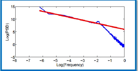
Kobayashi and Musha [18] first reported the frequency dependence of thepower spectrum of RR interval fluctuations. The plots had an uneven densitythat might overweight for data in the higher-frequency range. Therefore, alogarithmic interpolation is used, resulting in a balanced number of pointsforlinear interpolation. The slope of the regression line of the log(power) versuslog(frequency) relation (1/f), usually calculated in the 10-4 –10-2Hz frequencyrange, corresponds to the negative scaling exponent ß and provides an index forlong-term scaling characteristics [19]. Fig.3 indicates the (1/f)ßrelationbetween PSD and frequency, reflected on a log–log scale approximately as a line.The figure is the result for the example used throughout this chapter, leading toa 1/f slope of -1.34.
Figure 3 Log(power) versus log(frequency) plot of the tachogram example given in (Fig.1). The thick line indicates the 1/f slope or scaling exponent ß and is derived asthe regression line calculated in the 10-4–10-2Hz
frequency range.
This broadband spectrum, characterizing mainly slow HR fluctuations indicatesa fractal-like process with a long-term dependence [20]. Saul et al [19] foundthat ß is similar to -1 in healthy young men. This linearity of the regression lineand the slope of -1 in healthy persons mean that the plots of RR-interval versustime over 2 minutes (10-2Hz), 20 minutes (10-3Hz) and 3 hours (10-4Hz) mayappear similar. This is called scale-invariance or self-similarity in fractal theory. Ithas been suggested that the scale invariance may be a common feature of normalphysiological function. The breakdown of normal physiological functioning couldlead to either random or periodic behavior, indicated by steeper 1/fslopes, whichcould lead to a more vulnerable state of homeostasis.Bigger et al [21] reported an altered regression line (ß ≈ - 1.15) in patients afterMI. A disadvantage of this measure is the need for large datasets. Moreover,stationarity is not guaranteed in long datasets and artefacts and patient movementinfluence spectral components.
3.2 Fractal dimension
3.2.1 Algorithm of Katz
According to the method of Katz [23] the FD of a curve can be defined as
𝐷𝐾𝑎𝑡𝑧 =log (𝐿)
log (𝑑) (1)
where L is the total length of the curve or sum of distances between successivepoints, and d is the diameter estimated as the distance between the first point ofthe sequence and the most distal point of the sequence. Mathematically, d can beexpressed as:
𝑑 = max 𝑥 1 − 𝑥 𝑖 ∀𝑖 (2)
Figure 4 An illustration of how fractals look like with the feature of scaleindependence and self-similarity: (a) the Koch curve and (b and
c) details of the topof the curve.
Considering the distance between each point of the sequence and the first, pointi is the one that maximizes the distance with respect to the first point. The FDcompares the actual number of units that compose a curve with the minimumnumber of units required to reproduce a pattern of the same spatial extent. FDscomputed in this fashion depend upon the measurement units used. If the unitsare different, then so are the FDs. Katz approach solves this problem by creating ageneral unit or yardstick: the average step or average distance between successivepoints, a. Normalizing the distances, Dkatzis then given by
𝐹𝐷 =log (
𝐿 𝑎)
log (𝑑𝑎) (3)
3.2.2 Box-counting method
What is the relationship between an objects length (or area or volume) and itsdiameter? The answer to this question leads to another way to think aboutdimension. Let us consider a few examples (Fig.5). If one tries to coverthe unit square with little squares of side length ϵ, one will need 1/ϵ2boxes. Tocover a segment of length 1, you only need 1/ ϵ little squares. If the little cubes are used to cover a1x1x1 cube, 1/ ϵ3
is needed. Note that the exponent here is the same asthe dimension. This is no coincidence, but thegeneral rule is:
Figure 5 Principle of box-counting algorithm [25].
where o is the length of a box or square, S the full dataset and N o (S) the minimumnumber of n-dimensional boxes needed to cover S fully. d is the dimension of S.This way, the FD can be estimated via a box-counting algorithm as proposed byBarabasi and Stanley [24] as follows:
𝐹𝐷 = lim∈→0ln 𝑁ln∈∈(𝑆) (5)
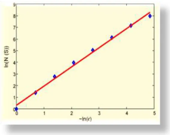
One also refers to the fractal dimension as the box-counting dimension or shortlybox dimension. Given the standard RR interval time series as example(Fig. 1), the relation between the number of boxes and the box size is shown in (Fig. 6), resulting in a FD equal to 1.6443.
Figure 6Illustration of the box-counting method applied on the tachogram examplegiven in (Fig.1). First a 2D plane is built based on the dataset S, here consisting ofboth the RR intervals and corresponding time points. The number of boxes in that planecontaining points of the dataset is counted and given by Nϵ(S). This
depends on the sizeof the boxes, namely ϵ. This relation is represented in a ln – ln scale by the rhombuses.The line is the best fit through these points and the slope of the line reflects the fractaldimension.
3.3 Detrended fluctuation analysis
Detrended fluctuation analysis (DFA) is used to quantify the fractal scalingproperties of short interval signals. This technique is a modification of root-meansquareanalysis of random walks applied to nonstationary signals [26]. The rootmeansquare fluctuation of an integrated and detrended time series is measuredat different observation windows and plotted against the size of the observationwindow on a log- log scale. First, the RR interval time series x (of total lengthN) is integrated as follows:
𝑦 𝑘 = 𝑘𝑖=1 𝑥 𝑖 − 𝑥𝑎𝑣𝑒𝑟𝑎𝑔𝑒 (6)
where y(k) is the kthvalue of the integrated series, x(i) is the ithRRintervaland x average is the mean of the RR intervals over the entire series. Then, theintegrated time series is divided into windows of equal length n. In each windowof length n, a least-squares line is fitted to the data, representing the trend in thatwindow as shown in (Fig.7(a)). The y-coordinate of the straight line segmentsare denoted by yn(k). Next, the integrated time series is detrended, yn (k), in eachwindow. The rootmeansquare fluctuation of this integrated and detrendedseriesis calculated using the equation:
Figure 7 The principle of detrended fluctuation analysis (DFA).
This computation is repeated over all time scales (window sizes) to obtain therelationship between F(n) and the window size n (the number of points, hereRR intervals, in the window of observation). Typically, F(n) will increase withwindow size. The scaling exponent DFA a indicates the slope of this line, whichrelateslog(fluctuation) to log(window size) as visualized in (Fig.7(b)). Thismethod, based on a modified random walk analysis, was introduced and applied tophysiological time series by Peng et al [27]. It quantifies the presence or absenceof fractal correlation properties in nonstationary time series data. DFA usuallyinvolves the estimation of a short-term fractal scaling exponent 𝛼1over the rangeof 4 ≤ n ≤16 heart beats and a long-term
scaling exponent𝛼2 over the range of16 ≤ n ≤ 64 heart beats. Figure 7(b) shows the DFA plot for the HR example,where DFA 𝛼1 is 1.0461 and DFA 𝛼2 is 0.8418.
Healthy subjects revealed a scaling exponent of approximately 1, indicating fractallikebehavior. Patients with cardiovascular disease showed reduced scalingexponents, suggesting a loss of fractal-like HR dynamics (𝛼1< 0.85 [28];𝛼1< 0.75 [26]). From many studies on test signals, one had the following a ranges:
• 0 < α < 0.5: power-law anti-correlations are present such that large valuesare more likely to be followed by small values and vice versa.
• α = 0.5: indicates white noise.
• 0.5 < α < 1: power-law correlations are present such that large values aremore likely to be followed by large values and vice versa. The correlation isexponential.
• α = 1: special case corresponding to 1/f noise.
• α> 1: correlations exist, but cease to be of a power-law form. • α = 1.5: indicates Brownian noise.
The a exponent can also be viewed as an indicator of the ’roughness’ of the originaltime series: the larger the value of a, the smoother the time series. In this context,1/fnoise can be interpreted as a compromise or ’tradeoff’ between the completeunpredictability of white noise (very rough ’landscape’) and the much smootherlandscape of Brownian noise.
It is important to note that DFA can only be applied reliably on time series of atleast 2000 data points. DFA as such is a mono-fractal method, but also multi-fractalanalysis exists [29]. This multifractal analysis describes signals that are morecomplex than those fully characterized by a mono-fractal model, but it requiresmany local and theoretically infinite exponents to fully characterize their scalingproperties.
3.4 Approximate entropy and sample entropy
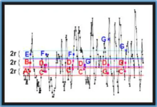
specifically, itmeasures the likelihood that runs of patterns that are close will remain close forsubsequent incremental comparisons. An intuitive presentation is shown in (Fig. 8).It was calculated according to the formula of Pincus [30]:
𝐴𝑝𝐸𝑛 𝑚, 𝑟, 𝑁 =𝑁−𝑚+11 log 𝐶𝑖𝑚 𝑟 − 1 𝑁−𝑚 𝑁−𝑚 +1
𝑖=1 𝑁−𝑚𝑖=1 log 𝐶𝑖𝑚 𝑟 (8)
where
𝐶𝑖𝑚 𝑟 =𝑁−𝑚+11 𝑁−𝑚 +1𝑗 =1 𝜃(𝑟 − 𝑥𝑖− 𝑥𝑗 ) (9)
is the correlation integral with θtheHeavyside step function. xi and xjarerespectively the ithandjthRR interval from the tachogram of length N. Thevalues of the input variables are chosen fixed, namely m = 2 and r = 0.2 assuggested by Goldberger et al[31] (m being the length of compared runs and rthe tolerance level). High values of ApEn indicate high irregularity and complexityin time-series data.
Sample Entropy (SampEn) was developed by Richman and Moorman [32] andis very similar to the ApEn, but there is a small computational difference. InApEn, the comparison between the template vector and the rest of the vectorsalso includes comparison with itself. This guarantees that probabilities 𝐶𝑖𝑚 𝑟 arenever zero.Consequently, it is always possible to take a logarithm of probabilities.Because template comparisons with itself lower ApEn values, the signals areinterpreted to be more regular than they actually are. These selfmatchesarenot included in SampEn leading to probabilities 𝐶𝑖′𝑚 𝑟 :
𝐶𝑖′𝑚 𝑟 =𝑁−𝑚 +11 𝑁−𝑚 +1𝑗 =1 𝜃(𝑟 − 𝑥𝑖 − 𝑥𝑗 )𝑗 ≠ 𝑖(10)
Finally, sample entropy is defined as:
𝑆𝑎𝑚𝑝𝐸𝑛 𝑚, 𝑟, 𝑁 = − ln[𝜑𝜑′𝑚 +1′𝑚 𝑟 𝑟 ] (11)
SampEn measures the complexity of the signal in the same manner as ApEn.However, the dependence on the parameters N (number of points) and r is different. SampEn decreases monotonically when r increases. In theory, SampEndoes not depend on N where ApEn does. In analyzing time series including <200data points, however, the confidence interval of the results is unacceptably large.For entropy measures, stationarity is required. In addition, outliers such as missedbeats and artefacts may affect the entropy values.The sample entropy of the tachogram example given in (Fig.1) is 4.4837.
Figure 8. Intuitive presentation of the principle of Approximate Entropy (ApEn) andSample Entropy (SampEn). For a twodimensional vector AB, the tolerance level r canbe represented by horizontal red and violet lines around point A and B respectively, withwidth of 2r · SD. Then all vectors, say CD, whose first and
second points (respectivelyC and D) are within the tolerance ranges of A and B (±r · SD), are counted to measurewithin a tolerance level r the regularity, or frequency, of patterns similarly to a givenpattern of AB.
In the figure, five CD vectors are close to vector AB. When increasingvector dimension from 2 to 3 (ABE), two vectors, namely CDF, remain close while theother three vectors, CDG, show emerging patterns. Thus the
likelihood of remaining closeis about 2/5. It is clear that such likelihood tends to 1 for regular series, and producesApEn = 0 when taking the logarithm, while it tends to 0 for white noise and results ininfiniteApEn
theoretically. From [33].
3.5 Correlation dimension
space. For every possible state of the system, orallowed combination of values of the system’s parameters, a point is plotted in themultidimensional space. Often this succession of plotted points is analogous to thesystem’s state evolving over time. In the end, the phase space represents all thatthe system can be, and its shape can easily elucidate qualities of the system thatmight not be obvious otherwise. A phase space may contain many dimensions.The correlation dimension (CD) can be considered as a measure for the number ofindependent variables needed to define the total system, here the cardiovascularsystem generating the RR interval time series, in phase space [34].
Before explaining how CD is calculated from a tachogram, the terms attractor,trajectory and attractor reconstruction has to be clarified. An attractor is a settowards which a dynamical system evolves over time. That is, points that get closeenough to the attractor remain close even if slightly disturbed. Geometrically,an attractor can be a point, a curve, a surface (called a manifold), or even acomplicated set with a fractal structure known as a strange attractor. Describingthe attractors of chaotic dynamical systems has been one of the achievements ofchaos theory. A trajectory of the dynamical system in the attractor does nothave to satisfy any special constraints except for remaining on the attractor. Thetrajectory may be periodic or chaotic or of any other type. For experimental andnaturally occurring chaotic dynamical systems as the cardiovascular system is,the phase space and a mathematical description of the system are often unknown.Attractor reconstruction methods have been developed as a means to reconstructthe phase space and develop new predictive models. One or more signals from thesystem, here the RR interval time series reflecting heart rate, must be observedas a function of time. The time series are then used to build an approach of theobserved states.
Correlation dimension analysis of HRV signals is based on the method ofGrassberger and Procaccia [35]. As always, we start with a tachogram or RRinterval time series x(t) of data points xi = x(ti) and i = 1 . . . N (the numberof heart beats in the signal)(Fig.1). Next, an attractor reconstruction takesplace. The reconstructed trajectory, X, can be expressed as a matrix where eachrow is a phase space vector, X = (x1 x2 . . . xM )T. For a time series of length N,{x1 , x2 , . . . , xN }, each xi is given by xi = (xi , xi+τ , xi+2τ , . . . , xi+(m-1)τ ).
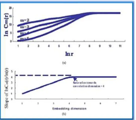
The parameters m and τ are respectively called the embedding dimension and thetime delay. The time delay for the CD is the value of the first zero crossing ofthe normalized (mean = 0 and standard deviation = 1) autocorrelation functionof the time series and the time axis. The embedding dimension is usually variedincreasingly between the values 2 and 30. The distances between the reconstructedtrajectories xi and xj (i, j = 1 . . . N and i< j) are calculated and the total rangeof these distances is divided into discrete intervals, presented by r. Based on thesedistances, the correlation integral 𝐶𝑚 𝑟 , as already defined in equation (9), iscalculated as a function of r and this for successive values of m. As for a chaoticsignal the relation 𝐶𝑚 𝑟 ~ 𝑟𝐶𝐷holds, CD can derived by plotting 𝐶𝑚 𝑟 versusr in a ln – ln scale. This is visualized in (Fig.9(a))
for different values ofthe embedding dimension m. Next, calculating the slope of such a curve resultstheoretically in the CD, but as can be seen in the figure, this slope depends on thechoice of m. In fact, the slope becomes steeper as m increases but will saturate ata certain level of the embedding dimension. Therefore, the slope can be plottedas a function of this embedding dimension m which makes it possible to see fromwhich m on the slope is saturated. As shown in (Fig.9(b)), the point on they and xaxis where this curve (slope versus m) saturates is called respectively thecorrelation dimension CD and the embedding dimension of the time series. Although the algorithm of Grassberger and Procaccia [35] is often used, it hasseveral limitations such as the sensitivity to the length of the data, the unclearrange of embedding dimensions to consider and the lack of having a confidenceinterval. To solve these problems, Judd [36] developed another algorithm toestimate the CD in a more robust way, which was used in this thesis. The CD for the (fig. 2) is 3.61 and for the tachogram example given in (Fig.1) is 3.7025.
When a finite value is found for the CD of a time series, correlations are presentin the signal. To conclude whether these correlations are linear or nonlinear, asurrogate time series needs to be calculated. A significant difference between theCD of the surrogate and the original time series indicates that there are nonlinearcorrelations present in the signal. The significance level is calculated as: 𝑆 = 𝐶𝐷𝑠𝑢𝑟𝑟 − 𝐶𝐷𝑑𝑎𝑡𝑎 /
𝑆𝐷𝑠𝑢𝑟𝑟. A value of S > 2 indicates that the measure reflectsnonlinear correlations within the time series. In case
of S > 2 the signal canbe chaotic, but this is not absolutely sure unless other nonlinear parameters likee.g. Lyapunov exponents are available and positive values found. With S < 2 nosignificant difference is found between the two time series, the signal is not chaotic.
3.6 Lyapunov exponent
space follow typical patterns.Closely spaced trajectories converge and divergeexponentially, relative to each other. For dynamicalsystems, sensitivity to initial conditions is quantified bytheLyapunov exponent (Λ). They characterize theaverage rate of divergence of these neighboring trajectories.A negative exponent implies that the orbitsapproach a common fixed point. A zero exponentmeans the orbits maintain their relative positions; theyare on a stable attractor. Finally, a positive exponentimplies the orbits are on a chaotic attractor [37].
Figure 9. Example of how to calculate the correlation dimension (CD). (a)Correlation integral 𝑪𝒎 𝒓 as function of the tolerance level r for different choices ofthe embedding dimension m. As 𝑪𝒎 𝒓 ~ 𝒓𝑪𝑫, the slope of such curve in a ln – ln scaleresults theoretically in the correlation dimension CD, but depends on m.
(b) Plot of theslopes of ln 𝑪𝒎 𝒓 / 𝐥𝐧(𝒓) as function of m.
3.6.1 Wolf’s Algorithm
Wolf’s algorithm is straightforward and uses the formulas defining the system. It calculates two trajectories in thesystem, each initially separated by a very small interval R0 . The first trajectory is taken as a reference, or ’fiducial’trajectory, while the second is considered ’perturbed’. Both are iterated together until their separation abs(R1 - R0)is large enough, at which point an estimate of the Largest Lyapunov Exponent LLE can be calculated asΛ𝐿=Δ1𝑡log2𝑎𝑏𝑠 (𝑅𝑅1
0). The perturbedtrajectory is then moved back to a separation of sign(R1)R0 towards the fiducial, and the process repeated. Over time,a running average of ΛL will converge towards the actual LLE [38]. The normal HR signal shown in (Fig. 2) has LLE equal 0.505Hz.
3.6.2 Rosenstein algorithm
The first step of this approach involves reconstructing the attractor dynamicsfrom the RR interval time series. The method of delays is used which is alreadydescribed in detail when explaining the correlation dimension. After reconstructingthe dynamics, the algorithm locates the nearest neighbor of each point on thetrajectory. The nearest neighbor, x'j , is found by searching for the point thatminimizes the distance to the particular reference point, xj . This is expressed as:
𝑑𝑗 0 = min||𝑥𝑗− 𝑥𝑗/|| ∀𝑥𝑗/(12)
where𝑑𝑗 0 is the initial distance from the 𝑗𝑡ℎ point to its nearest neighbor and || ... || denotes the Euclidean norm. An additional constraint is imposed, namely that nearest neighbors have a temporal separation greater than the mean period of the RR interval time series. Therefore, one can consider each pair of neighbors as the nearby SD initial conditions for different trajectories. The LLE is then estimated as the mean rate of the SD separation of the nearest neighbors. More concrete, it is assumed that the 𝑗𝑡ℎ pair of nearest neighbors diverge approximately at a rate given by the LLE ΛL:
𝑑𝑗(𝑗) ≈ 𝑑𝑗(0)𝑒Λ(𝑖.∆𝑡) (13)
By taking the ln of both sides of this equation:
which represents a set of approximately parallel lines (for j = 1, 2, . . . ,J), each with a slope roughly proportional to the ΛL.
The natural logarithm of the divergence of the nearest neighbor to the jthpoint in the phase space is presented as a function of time. The LLE is then calculated as the slope of the least squares fit to the ’average’ line defined by:
Λ𝐿 𝑡 =∆𝑡1 ln 𝑑𝑗(𝑡) (15)
where ln 𝑑𝑗(𝑡) represents the mean logarithmic divergence over all values of j for all pairs of nearest neighbors
over time. This process of averaging is the key to calculating accurate values for the LLEusing smaller and noisy data sets compared to other algorithms [39]. The LLE computed using the Rosenstein algorithm is 0.7586 Hz for the HR signal shown in (Fig. 2).
3.6.3. The Mazhar-Eslam Algorithm
The Mazhar-Eslam [3, 40] algorithm uses Discrete Wavelet Transform (DWT) considering the merits of DWT over that of FFT. Although the FFT has been studied extensively, there are still some desired properties that are not provided by FFT. There are some points are lead to choose DWT instead of FFT. The first point is hardness of FFT algorithm pruning. When the number of input points or output points are small comparing to the length of the DWT, a special technique called pruning is often used [41]. However, it is often required that those zero input data are grouped together. FFT pruning algorithms does not work well when the few non-zero inputs are randomly located. In other words, sparse signal does not give rise to faster algorithm.
The other disadvantages of FFT are its speed and accuracy. All parts of FFT structure are one unit and they are in an equal importance. Thus, it is hard to decide which part of the FFT structure to omit when error occurring and the speed is crucial. In other words, the FFT is a single speed and single accuracy algorithm, which is not suitable for SED cases.
The other reason for not selecting FFT is that there is no built-in noise reduction capacity. Therefore, it is not useful to be used. According to the previous ,the DWT is better than FFT especially in the SED calculations used in HRV, because each small variant in HRV indicates the important data and information. Thus, all variants in HRV should be calculated.
The Mazhar-Eslam algorithm depends to some extend on Rosenstein algorithm’s strategies to estimate lag and mean period, and uses the Wolf algorithm for calculating the MVF (Ω𝑀) except the first two steps, whereas the final steps are taken from Rosenstein’s method. Since the MVF (Ω𝑀) measures the degree of the SED
separation between infinitesimally close trajectories in phase space, as discussed before, the MVF (Ω𝑀) allows
determining additional invariants. Consequently, the Mazhar-Eslam algorithm allows to calculate a mean value for the MVF (Ω𝑀), that is given by
Ω𝑀
= Ω𝑀 𝑖 𝑗 𝑗
𝑖=1 (16)
Note that the Ω𝑀𝑖s contain the largest Ω𝑀𝐿 and variants Ω𝑀s that indicate to the helpful and important data.
Therefore, the Mazhar-Eslam algorithm is a more SED prediction quantitative measure. Therefore, it is robust quantitative predictor for real time, in addition to its sensitivity for all time whatever the period.
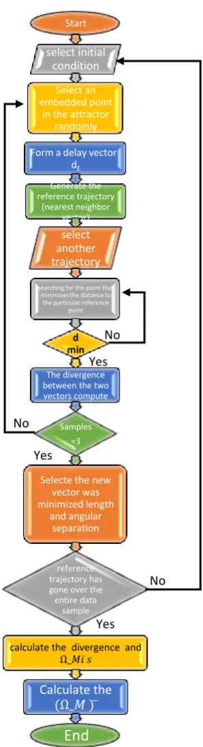
Apply the Mazhar-Eslam algorithm to the HRV of the normal case given in (Fig. 2), it is found that the mean MVF (Ω 𝑀 ) as 0.4986 Hz, which is more accurate than Wolf (0.505 Hz) and Rosenstein (0.7586 Hz).Figure10.shows the flowchart for calculating the Mazhar-Eslam MVF algorithm.
Figure10.shows the flowchart steps for calculating the Mazhar-Eslam MVFM algorithm. First Start to select an initial condition. An embedded point in the attractor was randomly selected, which was a delay vector with dE elements. A delay vector generates the reference trajectory (nearest neighbor vector). Then another trajectory is selected by searching for the point that minimizes the distance to the particular reference point. After thatthe divergence between the two vectors is computed. A new neighbour vector was consideredas the evolution time was higher than three sample intervals. The new vector was selected to minimize the length and angular separation with the evolved vector on the reference trajectory.The steps are repeated until the reference trajectory has gone over the entire data sample. The divergence and Ω𝐿𝑖𝑠 are calculated. Consequently,theΩ𝑀 is
Start
select initial condition
Select an embedded point
in the attractor randomly
Form a delay vector dE
Generate the reference trajectory
(nearest neighbor vector(
select another trajectory
searching for the point that minimizes the distance to
the particular reference point
d min
The divergence between the two vectors compute
Samples =3
Selecte the new vector was minimized length
and angular separation
reference trajectory has gone over the entire data
sample
calculate the divergence and
Ω_𝑀𝑖 𝑠
Calculate the
Ω_𝑀 ) ̅
End
Figure 10The flowchart of the Mazhar-Eslam algorithm.
Table (1) shows the different results of the normal case among Mazhar-Eslam, Wolf, and Rosenstein algorithms. From this table it is seen that, the Rosenstein algorithm has the lowest SED because of its quite high error (D = 51.72 % ) comparing to the optimum, while the Wolf algorithm takes a computational place for SED (D = 1 % ). However, the Mazhar-Eslam algorithm shows more sensitivity (D = 0.28 %) than Wolf algorithm as shown in (Fig. 11). The patient case deviation D for normal HRV case is calculated as:
𝐷𝑒𝑣𝑖𝑎𝑡𝑖𝑜𝑛 𝐷 = |Ω𝑀 𝑛𝑜𝑟𝑚𝑎𝑙 −Ω𝑀𝑐𝑎𝑠𝑒|(17) the cases percentage deviation is to be calculated as:
𝐷% =𝑛𝑜𝑟𝑚𝑎𝑙𝐷 × 100% (18)
Yes Yes
No
No
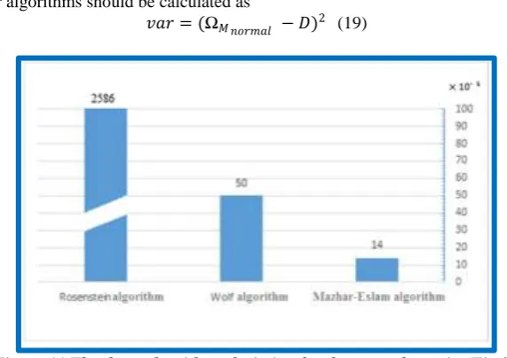
and, the variance for algorithms should be calculated as
𝑣𝑎𝑟 = (Ω𝑀 𝑛𝑜𝑟𝑚𝑎𝑙 − 𝐷)2 (19)
Figure 11 The three algorithms deviation for the normal case in (Fig.2).
The bar diagram in (Fig. 12) shows the percentage deviation of the three algorithms. From this figure it is seen that the Mazhar-Eslam algorithm gives the best result as it has the lowest percentage deviation (D = 14). At the same time, when calculating the variance to determine the accurate and best method, Mazhar-Eslam algorithm gives the best value. Figure 13.shows the bar diagram of the variance for normal control case using the HRV for Wolf, and Mazhar-Eslam algorithms. It is clear that the Mazhar-Eslam algorithm is more powerful and accurate than Wolf, because its variance better than Wolf by 0.0036. This result comes because the Mazhar-Eslam considers all the variability mean frequencies Ω 𝑀s unlike the Wolf method as it takes only the largest. Each interval of the HRV needs to be well monitored and taken into account because the variant in HRV is indication of cases.
Table 1The results of the three algorithms for the normal case shown in (Fig. 2)
Method parameter
Optimum Rosenstei n
Wolf
Mazhar-Eslam
ΩM 0.500000 0.758600 0.505000 0.498600 D 0.00000 0.258600 0.005000 0.001400 D% 0.000000 51.720000 1.000000 0.280000 Var 0.250000 0.058274 0.245025 0.248602
From the bar diagram in (Fig. 13) it is seen that the Mazahar-Eslam algorithm is most useful and sensitive comparing to Wolf and Rosenstein algorithms.
3.7 Hurst exponent (H)
The Hurst exponent is a measure that has been widelyused to evaluate the self-similarity and correlationproperties of fractional Brownian noise, the time seriesproduced by a fractional (fractal) Gaussian process.Hurst exponent is used to evaluate the presence orabsence of long-range dependence and its degree in atime series. However, local trends (nonstationarities) isoften present in physiological data and maycompromisethe ability of some methods to measure self-similarity.Hurst exponent is the measure of the smoothnessof a fractal time series based on the asymptotic behaviorof the rescaled range of the process. The Hurst exponentH is defined as:
Figure 12 The three algorithms Percentage deviation (D%) for the normal case (Fig. 2).
where T is the duration of the sample of data and R/Sthe corresponding value of rescaled range. The aboveexpression is obtained from the Hurst’s generalizedequation of time series that is also valid for Brownianmotion. If H = 0.5, the behavior of the time series issimilar to a random walk. If H < 0.5, the time -seriescover less ‘‘distance’’ than a random walk. But ifH> 0.5, the time-series covers more ‘‘distance’’ than arandom walk. H is related to the dimension CD givenby:
𝐻 = 𝐸 + 1 − 𝐶𝐷 (21)
where E is the Euclidean dimension.
Figure 13 The Variance of Wolf and Mazhar-Eslam algorithm for normal case (Fig.2).
For normal subjects, the FD is high due to thevariation being chaotic. And for Complete Heart Block(CHB) and Ischemic/dilated cardiomyopathy, this FD decreases because theRR variation is low. And for AF and SSS, this FDvalue falls further, because the RR variation becomeserratic or periodic respectively [42]. The H is 0.611 forthe HR signal shown in (Fig. 2).
0 10 20 30 40 50 60
Mazhar-Eslam Wolf
Rosenstein
D%
0.243 0.244 0.245 0.246 0.247 0.248 0.249
Mazhar-Eslam Wolf
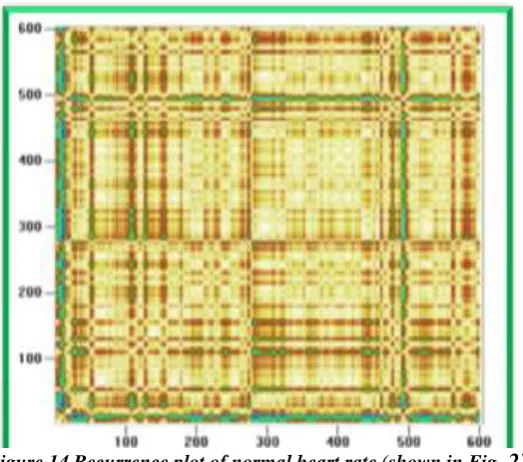
Figure 14 Recurrence plot of normal heart rate (shown in Fig
. 2)
3.8 Recurrence plots
In time-series analysis, the dynamic properties of thedata under consideration are relevant and valid only, ifthe data is stationary. Recurrence plots (RP) are used torevealnonstationarity of the series. These plots werefirst proposed by Eckmann et al. [43]as graphical toolfor the diagnosis of drift and hidden periodicities in thetime evolution, which are unnoticeable otherwise. Abrief description on the construction of recurrenceplots is described below.
Let xi be the i th
point on the orbit in an m-dimensionalspace. The recurrence plot is an array of dots in an𝑁 × 𝑁square, where a dot is placed at (i,j)whenever xjissufficiently close to xi . To obtain the recurrence plot, mdimensionalorbit of xi is constructed. A radius r suchthat the ball of radius r centered at xi inℜ𝑚contains areasonable number of other points xj of the orbit. Finally,a dot is plotted for each point (i,j) for which xj is in theball of radius r centered at xi. The plot thus obtained isthe recurrence plot. The plots will be symmetric alongthe diagonal i = j, because if xi is close to xj, then xjisclose to xi . The recurrence plot of normal HR (shown inFig. 2) is given in (Fig. 14). For normal cases, the RP hasdiagonal line and less squares indicating more variationindicating high variation in the HR. Abnormalities likeCHB and in Ischemic/dilated cardiomyopathy cases,show more squares in the plot indicating the inherentperiodicity and the lower HR variation [44].
IV.
Conclusion
This review introduces the mathematics and techniques, necessary for a good understandingof the methodology used in HRV analysis. After the peak detection algorithm andthe preprocessing methods, the linear methods in time domain, frequency domainand the time-frequency representations were represented. Also an overview ofsome nonlinear techniques assessing scaling behavior, complexity and chaoticbehavior were given.
References
[1]
Reed MJ, Robertson CE and Addison PS. 2005 Heart rate variability measurements and the prediction of ventricular arrhythmias. Q J Med; 98:87-95.[2]
Task Force of the European Society of Cardiology and the North AmericanSociety of Pacing and Electrophysiology. Heart rate variability: standardsof measurement, physiological interpretation and clinical use. Circulation,93:1043–1065, 1996.[3]
MAZHAR B. TAYEL, ESLAM I. ALSABA. "Robust and Sensitive Method of Lyapunov Exponent for Heart Rate Variability". InternationalJournal of Biomedical Engineering and Science (IJBES), Vol. 2, No. 3, July 2015. pp 31 -48[4]
Conny MA, Arts VR, Kollee LAA, Hopman JCW, Stoelinga GBA, Geijn HPV. 1993 Heart rate variability. Ann Int Med 118(6):436-447.[6]
Davidson NS, goldner S, McCloskey DI. 1976 Respiratory modulation of baroreceptor and chemoreceptor reflexes affecting heart rate and cardiac vagal efferent nerve activity. J Physiol (London); 259:523-530.[7]
McCabe PM, Yongue BG, Ackles PK, Porges SW. 1985 Changes in heart period, heart period variability and a spectral analysis estimate of respiratory sinus arrhythmia in response to pharmacological manipulations of the baroreceptor reflex in cats. Psychophysiology; 22:195203.[8]
Pomeranz B, Macauley RJ, Caudill MA et al. 1985 Assessment of autonomic function in humans byheart rate spectral analysis. Am J Physiol; 248:H151-153.
[9]
D.J. Christini, K.M. Stein, S.M. Markowitz, S. Mittal, D.J. Slotwiner, M.A.Scheiner, S. Iwai, and B.B. Lerman. Nonlinear-dynamical arrhythmia controlin humans. Proceedings of the National Academy of Sciences of the UnitedStates of America, 98(10):5827–5832, 2001.[10]
J.F. Zbilut, N. Thomasson, and C.L. Webber. Recurrence quantificationanalysis as a tool for nonlinear exploration of nonstationary cardiac signals.Medical Engineering & Physics, 24(1):53–60, 2002.[11]
S. C. Malpas, "Neural influences on cardiovascular variability: possibilities andpitfalls,AmericanJournal of Physiology. Heart and Circulatory Physiology, vol. 282, pp. H6-20, Jan 2002.
![Figure 1 Thetachogram used as example [2].](https://thumb-us.123doks.com/thumbv2/123dok_us/1994759.1658835/1.595.166.429.520.671/figure-thetachogram-used-as-example.webp)
![Figure 2Heart rate variation of a normal subject [3].](https://thumb-us.123doks.com/thumbv2/123dok_us/1994759.1658835/2.595.177.424.107.244/figure-heart-rate-variation-normal-subject.webp)