Image Denoising via Robust Simultaneous Sparse Coding

(1)

Image Denoising via Robust Simultaneous Sparse

Coding

Lei Li

School of Technology, Beijing Forestry University, Beijing 100083, P. R. China Email:[email protected]

Jiangming Kan

Wenbin Li

Abstract—Simultaneous sparse coding (SSC) has shown great potential in image denoising, because it exploits dependencies of patches in nature images. However, imposing joint sparsity might neglect the sight difference between patches. In this paper, we propose an image denoising algorithm based on robust simultaneous sparse coding (RSSC). In our algorithm, the sparse coefficient matrix is decomposed into two parts. One coefficient matrix is imposed on the joint sparse regularizer which exploits self-similarities of image patches while the other matrix is imposed by the elementwise sparse regularizer which considers the subtle differences between patches. Experiments on the benchmark data show the superior performance over the state-of-art algorithms.

Index Terms—Image denoising, robust simultaneous sparse coding, regularization, accelerated proximal gradient (APG)

I. INTRODUCTION

In recent years, affordable hardware has made it possible for digital cameras to capture images of very high resolution. However, images are often corrupted by noise during the procedures of both image acquisition and transmission. An efficient denoising algorithm becomes very important to the performance of image processing techniques. Hence, denoising of images remains one of the most fundamental tasks of image processing. As follows, for an origin image

x R

∈

N and its degraded image

y

the problem of denoising can mathematically be defined as the following observation model:

i i i

y

= +

x

η

(1)

where

x

_i is the original pixel intensity of the

y

_i pixel observed as after being corrupted by zero mean independent identically distributed additive noise

η

_i .

recently,Many proposed denoising methods are based on image patches. Decomposing the origin image into overlapping patches, the data model can be written as

i

= +

i i

y

x

η

(2)

where

x

_i is the original image patch intensities with the -th pixel at its center written in a vectorized format and

i

y

is the observed patch corrupted by a noise vector

η

_i. Denoising an image is thus solving the inverse problem to estimate pixel intensities

x

_i.

In the past several decades, image denoising has been extensively studied and many algorithms [1] [2] [12] [13] have been proposed, leading to state-of-the-art performances. Of these various approaches, Non-Local Means (NLM) algorithm [1] recently proposed by Buades

et al. assumes that the noise is zero-mean and

uncorrelated across locations. Thanks to the presence of repeating structures in a given image, performing a weighted averaging of pixels with similar neighborhoods can suppress the noise. Inspired by the idea of NLM, Dabov et al. [2] proposed an effective algorithm named

BM3D. BM3D performs denoising by utilizing similar patches across the image in the transform domain rather than in the origin image space.

Recently, using redundant representations and sparsity for denoising of signals have drawn a lot of research attention [3] [4] [14]. In [3], Elad and Aharon applied the K-SVD algorithm to learn the optimal over-completed dictionaries for the observed noisy image. Each image patch can be sparsely represented by the learned dictionary and denoising is carried out by coding each patch as a linear combination of only a few atoms in the dictionary. Mairal et al. [4] extended the K-SVD

algorithm to the color image denoising.

However, in [3] [4], image patches are sparsely represented independently, which ignores self-similarities

(2)

in natural images as NLM did. Mairal et al. [5] argued

exploiting similarities can improve the denoising performance. And he grouped image patches into a few groups and argued patches in the same group have similar sparse decomposition. And the simultaneous sparse coding (SSC) is applied to learn the sparse representation matrix. Experiments show the superior performance over the K-SVD algorithm. Dong et al. [6] propose a new

denoising algorithm based on clustering-based sparse representation (CSR), which incorporates the dictionary learning and structural clustering into a unified variational framework.

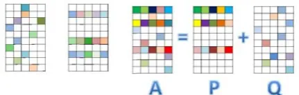
However, there is a key problem that similar patches corrupted by noises might not share the same structure and imposing joint sparse regularizer as done in [5] may degrade the denoising performance [7] [8]. To overcome this problem, in this paper, we propose our image denoising algorithm based on robust simultaneous sparse coding (RSSC). As shown in Fig.1, in our algorithm, the sparse coefficient matrix

A

is decomposed into two parts

P

,

Q

. A joint sparse regularizer is imposed on

P

, corresponding to the shared structure while an elementwise sparse regularizer is imposed on

Q

which corresponds to the non-shared features. The joint-sparsity exploits the similarities between patches while the elementwise sparsity considers the differences of patches. Experiments with images corrupted by synthetic noise show that the proposed method outperforms the state of the art algorithms in image denoising.

The rest of this paper is organized as follows. In Sec.2, our new image denoising algorithm is described in detail. Experimental results and comparison with other state-of-the-art approaches are presented in Sec.3. Our work is summarized in Sec.4.

II.ROBUSTSPARSEREPRESENTATIONMODEL

A. Image Denoising Model

Various image restoration tasks based on sparse coding can be formulated into the following minimization problem:

2

2 1

arg min

i

=

i

−

i

+

γ

i α

α

y

D

α

(3)

where

y = R x

_i _i denotes an degraded image patch of size

n

⋅

n

extracted at location

i

,

R

_i is the matrix

extracting patch

y

_i from

y

at location

i

and

n K×

∈

D R

is a fixed dictionary and

K

is its size,

K i

∈

α

R

is the reconstruction coefficients,

γ

is the penalty to control the sparsity of

α

_i. After determining sparse coefficients

α

_i , we estimate the original image

x

by solving the following over-determined system:

2 2

x

arg min

ij ij

ij

λ

=

−

+

∑

−

x

y x

R x D

α

(4)

This above quadratic equation has a straightforward solution:

1

T T

ij ij ij ij

ij ij

λ

−

⎛

⎞ ⎛

⎞

=

_⎜

+

_{⎟ ⎜}

+

_⎟

⎝

∑

⎠ ⎝

∑

⎠

x

I

R R

y

R D

α

(5)

A major drawback of (3) is that image patches are sparsely represented independently and dependencies between patches are ignored. The self-similarities among patches can be used to improve learned sparse models [5]. The basic idea is to group a set of similar

patches

[

₁

,

₂

, ,

]

n m

m

×

=

∈

Y

y y

"

y

R

and imposing a

grouped-sparsity regularizer on the matrix

[

1

, ...,

2 _m

]

=

A

α α

α

and (3) is reformulated as follows:

2

, A

1 arg min

2

F

λ

p q

=

−

+

A

Y DA

A

(6)

where

m

is the number of similar patches and

⋅

_{p q}_, is the pseudo-matrix norm defined as

, 1 n _p

i p q q

i=

=

∑

A

α

(7)

where i

[

₁

,...,

]

i im

α

=

α

denotes the

i

-th row of matrix

A

. In this paper, we choose the pair (

p

,

q

) with the values (1, 2). From (6), we can see that simultaneous sparse coding encourages similar patches to be represented by the same atoms and this can exploit the dependencies between patches.

However, due to image patches corrupted by noise, similar patches may not fall into a single shared structure [7] and block

A

₁₂ regularization might perform worse than simple separate elementwise

A

₁₁ regularization. Therefore, to deal with this problem, we propose our image denoising model based on robust sparse coding (RSC) as follows:

(

)

2 ,

1 1,2 2 1,1

1 ,

arg min

-2

F

λ

=

+

P Q

P Q

Y D P Q

P

Q

(8)

Figure 1. Illustration of sparsity vs. joint sparsity vs. robust joint sparsity: color squares represent nonzero values in the coefficient

(3)

where

P

is a group sparse component which reflects the same structure shared by similar patches and

Q

is an elementwise component which reflects the difference between patches. That is, we decompose the coefficient matrix into two components and impose different regularizer on them. This exploits the similarities between patches while considering their differences.

B. Optimization Algorithm

In this section, we show how to solve the robust image denoising model in (8) efficiently. Denote

(

)

(

)

(

)

2

1 1,2 2 1,1

1 F

,

2 G

,

F

λ

=

−

+

=

+

P Q

Y D P Q

P Q

P

Q

(9)

where

F

(

P Q

,

)

is the empirical loss function and

(

)

G

P Q

,

is the regularization term. Obviously, the object function in Problem (8) is a composite model, which is consist of a differential term

F

(

P Q

,

)

and a non-differential term

G

(

P Q

,

)

. And it can easily be proved

F

(

P Q

,

)

is jointly convex and

G

(

P Q

,

)

is also convex with respect to all their variables. Therefore, the global solution can be obtained. We propose a method based on the accelerated proximal gradient

(

APG

)

methods [9] [10] to solve the optimization problem. In the

APG

method [9] [10], at every iteration

k

, we need optimize the following problem:

(

)

_, _,

(

) (

)

,

argminT

k k

,

G ,

k k k

L

=

_{P Q}

+

P Q

P Q

(10)

where

(

)

(

)

(

)

(

)

, , , 2 2 T , 1

T , T , ,

2 T , , 2 2 k k k

k k k

L

k k k

k k F F L L ∂ = + − ∂ ∂ + − + − + − ∂ P Q P Q

P Q P Q P P

P

P Q

P P Q Q Q Q

Q

(11)

L

is the Lipschitz constant of

∂

T

(

,

)

∂

P Q

P

and

(

)

T

,

∂

P Q

Q

. And the initial

L

=

L

0

=

100

and is updated

L

_k

=

τ

L

_k₋₁ given

τ

> 1. The composite object function in Problem (8) has two nonsmooth functions. However, because they are separable, Problem (10) can be solved efficiently as the following two separate problems: 2 1 1 1,2 1 2 1,1

1

1 F

2

1

1 F

2

k k

k _F k

k k k k

L

λ

+ +

⎛

⎞

=

−

_⎜

−

∇

_⎟

+

⎝

⎠

⎛

⎞

=

−

_⎜

−

∇

_⎟

+

⎝

⎠

P Q

P

Q

(12)

where

∇

_P

F

and

∇

_Q

F

is the partial derivatives of

(

)

F

P Q

,

with respect to

P

and

Q

at

(

_{P Q}

k

,

k

)

.The above problems admit closed form solutions:

( )

1 1

1 2

max 0,1 , 1:

sign max 0,1

i i

k k

i k k

k k k

k i n L L λ λ + + ⎛ ⎞ ⎜ ⎟ = _⎜ − _⎟ ∀ = ⎜ ⎟ ⎝ ⎠ ⎛ ⎞ = _⎜ − _⎟ ⎝ ⎠ P u u

Q V V

(13)

Where k k

1 F

K

L

=

−

∇

_P

U

P

,

V

k

Q

k

1

_Q

F

k

L

=

−

∇

.

In [11], it has been proved the

APG

method achieves an

Ο

1

₂

k

⎛

⎞

⎜

⎟

⎝

⎠

residual from the optimal solution after

k

iterations. Finally, the algorithm for solving Problem (8) is given in Algorithm1.

Algorithm 1 Optimization for Problem (8)

- Input:

D

and

Y

.

- Output: Optimal solution

(

P Q

*

,

*

)

. (1).Set

1

_{= =0}

0

P P

,

Q Q

1

=

0

=0

,

t

₀

=

0

,

t

₁

=

1

,

k

=

1

,

0

100 L

=

L

=

,

η

=

1.05

,

λ

₁

=

0.3

,

λ

₂

=

0.01

. (2). while not converged do

(3). Compute the proximal points:

(

)

1

k

k k k k

v k

t

− −

−

=

+

−

P

;

(

)

1

k

k k k k

v k

t

− −

−

=

+

−

Q

;

(4). Calculate the gradient

∇

_P

F

,

∇

Q

F

;

(5). Calculate

_P

k+1

,

_Q

k+1_{via (13);}

(6).If

F

k1_, k1

T

k_, k_, k L

+ +

>

P Q P Q ,update

L

k

=

τ

L

k−1and go

to Step 5;

(7). Stepsize update:

( )

2

1

4

1

2

k k

t

+

=

(4)

III.IMAGE DENOISING EXPERIMENTS

We have implemented the proposed RSSC denoising algorithm under MATLAB. In all experiments, the block-size

n

=

64

, the penalties on sparsity

λ λ

₁

,

₂ are set as 0.5, 0.01 respectively. The dictionary is trained on patches from nature images and is shown in Fig 2. And the size of the dictionary

K

=

256

.

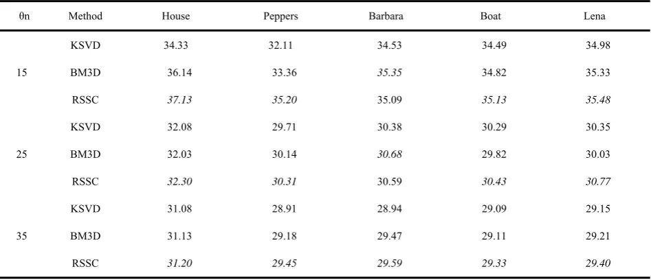
We first compare the proposed RSSC denoising algorithm and two leading methods for removing additive white Gaussian noise: K-SVD [3], BM3D [2]. The denoising results of all benchmark schemes are generated from the source codes or executables released by their authors. The PSNR performance of three competing denoising algorithms are reported in Table 1 (the highest PSNR value is in Italic).

From Table 1, we can see that our RSSC outperforms the other two algorithms on all tested images except that

BM3D achieves better performances on Barbara at the noise level

θ

n

=

15, 25

. Especially, when images are

corrupted by

θ

n

=

35

level Gauss noise, our algorithm

achieves the best results on all test images in the three ones. Therefore, we can conclude that RSSC outperforms the other two benchmark methods.

The visual comparison of the denoising methods is shown in Figs. 3-8. Fig. 5 presents visual results of different methods for Peper image with the noise level

25

n

θ

=

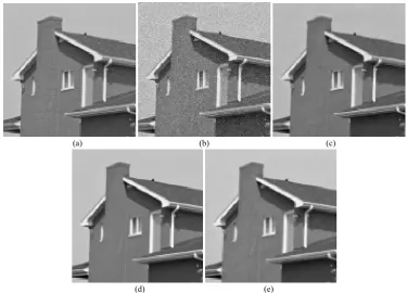
. We can observe that all methods can remove the noise effectively and our RSSC which exploits the similarities between patches and considering their differences provides an important improvement over the K-SVD method which considers each patch independently. The proposed method also outperforms over the BM3D method.

Fig. 6 gives the results of our algorithm on the corrupted image House. We can see that our RSSC method shows better visually quality result. The K-SVD method generates many visually disturbing artifacts in the denoised image. The BM3D method loses many details compared our RSSC method.

VI.CONCLUSION

In this paper, we propose a robust image denoising algorithm based on the robust simultaneous sparse coding. We decompose the sparse coefficient matrix into two halves. Joint sparsity regularizer is imposed on one matrix and elementwise sparsity regularizer is imposed on another. This makes our algorithm exploit the dependencies between patches while considering the differences between them. Experiments on the benchmark data show the superior performance over the state-of-art algorithms.

TABLE1.

QUANTITATIVE COMPARASION.THE GAUSS NOISE LEVEL ΘN=15,25,35 AND THE PSNR ARE CHOSEN AS THE PERFORMANCE MEASURE. BEST RESULTS ARE SHOWED IN ITALIC.

θn Method House Peppers Barbara Boat Lena

15

KSVD 34.33 32.11 34.53 34.49 34.98

BM3D 36.14 33.36 35.35 34.82 35.33

RSSC 37.13 35.20 35.09 35.13 35.48

25

KSVD 32.08 29.71 30.38 30.29 30.35

BM3D 32.03 30.14 30.68 29.82 30.03

RSSC 32.30 30.31 30.59 30.43 30.77

35

KSVD 31.08 28.91 28.94 29.09 29.15

BM3D 31.13 29.18 29.47 29.11 29.21

RSSC 31.20 29.45 29.59 29.33 29.40

(5)

(a) (b) (c)

(d) (e)

Figure 4. Denoising performance comparison for Boat image at Gauss noise level θn = 15. From the left to right, the original image, noising image, KSVD, BM3D, RSSC.

(a) (b) (c)

(d) (e)

(6)

(a) (b) (c)

(d) (e)

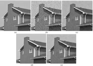
Figure 6. Denoising performance comparison for House image at Gauss noise level θn = 25. From the left to right, the original image, noising image, KSVD, BM3D, RSSC.

(a) (b) (c)

(d) (e)

(7)

(a) (b) (c)

(d) (e)

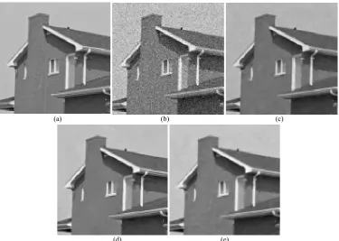
Figure 8. Denoising performance comparison for House image at Gauss noise level θn = 35. From the left to right, the original image, noising image, KSVD, BM3D, RSSC (a) (b) (c)

(d) (e)

(8)

ACKNOWLEDGMENT

This work was supported by the Fundamental Research Funds for the Central Universities (Grant No. BLYX200905 and TD2013-4) and National Natural Science Foundation of China (Grant No. 30901164).

REFERENCES

[1] A. Buades, B. Coll, and J. Morel, “A review of image denoising algorithms, with a new one,” Multiscale Modeling and Simulation, vol. 4, no. 2, pp. 490–530, 2005.

[2] K. Dabov, A. Foi, V. Katkovnik, and K. Egiazarian, “Image denoising by sparse 3-d transform-domain collaborative filtering,” IEEE Trans Image Processing, vol.

16,no. 8, pp. 2080–2095, 2007.

[3] M. Elad and M. Aharon, “Image denoising via sparse and redundant representations over learned dictionaries,” IEEE Trans Image Processing,, vol. 15, no. 12, pp.3736–3745,

2006.

[4] J. Mairal, M. Elad, and G. Sapiro, “Sparse representation for color image restoration,” IEEE Trans Image Processing,, vol. 17, no. 1, pp. 53–69, 2008.

[5] J. Mairal, F. Bach, J. Ponce, G. Sapiro, and A. Zisserman, “Non-local sparse models for image restoration,” in

Computer Vision, IEEE 12th International Conference on. IEEE, 2009, pp. 2272–2279.

[6] W. Dong, X. Li, D. Zhang, and G. Shi, “Sparsity-based image denoising via dictionary learning and structural clustering,” in Computer Vision and Pattern Recognition(CVPR), 2011 IEEE Conference on, 2011, pp.

457–464.

[7] A. Jalali, P. Ravikumar, S. Sanghavi, and C. Ruan, “A dirty model for multi-task learning,” Advances in Neural Information Processing Systems, vol. 23, pp. 964–972,

2010.

[8] S. Negahban and M. J. Wainwright, “Joint support recovery under high-dimensional scaling: Benefits and perils of l1,-regularization,” Advances in Neural Information Processing Systems, vol. 21, pp. 1161–1168,

2008.

[9] P. Tseng, “On Accelerated Proximal Gradient Methods for Convex-Concave Optimization,” unpublished.

[10]S. Ji and J. Ye, “An accelerated gradient method for trace norm minimization,” in International Conference on Machine Learning. ACM, 2009.

[11]P. Gong, J. Ye, and C. Zhang, “Robust multi-task feature learning,” in Proceedings of the 18th ACM SIGKDD international conference on Knowledge discovery and data mining, New York, NY, USA: ACM, pp. 895–903. 2012.

[12]G. Liu, J. Liu, Q. Wang, W. He, “The Translation Invariant Wavelet-based Contourlet Transform for Image Denoising,” Journal of Multimedia, North America, 7, jun.

2012.

[13]H. Fan, Y. Wang, J. Li, “Image Denoising Algorithm Based on Dyadic Contourlet Transform,” Journal of Software, North America, 6, jun. 2011.

[14]J. Hu, Y. Pu, J. Zhou, “A Novel Image Denoising Algorithm Based on Riemann-Liouville Definition,” Journal of Computers, North America, 6, jul. 2011.

Lei Li was born in JiLin Province, China, in 1980. He studies in Technology Beijing Forestry University, and separately gained a bachelor's degree in 2005 and a master's degree in 2008. Now, he is a doctorate candidate in the same university. His research interests mainly include information security, image processing image compression.

Jiangming Kan received in PhD degree in forestry engineering from Beijing Forestry University, P.R.China in 2009. Currently, he is an associate professor in Beijing Forestry University. His research interests include computer vision and intelligent control.