Atmos. Meas. Tech., 6, 661–675, 2013 www.atmos-meas-tech.net/6/661/2013/ doi:10.5194/amt-6-661-2013
© Author(s) 2013. CC Attribution 3.0 License.
EGU Journal Logos (RGB)
Advances in
Geosciences
Open Access
Natural Hazards
and Earth System
Sciences
Open AccessAnnales
Geophysicae
Open AccessNonlinear Processes
in Geophysics
Open AccessAtmospheric
Chemistry
and Physics
Open AccessAtmospheric
Chemistry
and Physics
Open Access DiscussionsAtmospheric
Measurement
Techniques
Open AccessAtmospheric
Measurement
Techniques
Open Access DiscussionsBiogeosciences
Open Access Open Access
Biogeosciences
DiscussionsClimate
of the Past
Open Access Open Access
Climate
of the Past
Discussions
Earth System
Dynamics
Open Access Open Access
Earth System
Dynamics
DiscussionsGeoscientific
Instrumentation
Methods and
Data Systems
Open Access
Geoscientific
Instrumentation
Methods and
Data Systems
Open Access DiscussionsGeoscientific
Model Development
Open Access Open Access
Geoscientific
Model Development
DiscussionsHydrology and
Earth System
Sciences
Open AccessHydrology and
Earth System
Sciences
Open Access DiscussionsOcean Science
Open Access Open Access
Ocean Science
Discussions
Solid Earth
Open Access Open Access
Solid Earth
Discussions
The Cryosphere
Open Access Open Access
The Cryosphere
Discussions
Natural Hazards
and Earth System
Sciences
Open Access
Discussions
Linearisation of the effects of spectral shift
and stretch in DOAS analysis
S. Beirle1, H. Sihler1,2, and T. Wagner1
1Max-Planck-Institut f¨ur Chemie, Mainz, Germany
2Institut f¨ur Umweltphysik, Universit¨at Heidelberg, Heidelberg, Germany
Correspondence to: S. Beirle ([email protected])
Received: 3 October 2012 – Published in Atmos. Meas. Tech. Discuss.: 21 November 2012 Revised: 13 February 2013 – Accepted: 20 February 2013 – Published: 13 March 2013
Abstract. Differential Optical Absorption Spectroscopy
(DOAS) is a widely used method to quantify atmospheric trace gases from spectroscopic measurements. While DOAS can, in principal, be described by a linear equation system, usually nonlinearities occur, in particular as a consequence of spectral misalignments.
Here we propose to linearise the effects of a spectral shift by including a “shift spectrum”, which is the first term of a Taylor expansion, as pseudo-absorber in the DOAS fit. The effects of a spectral stretch are considered as additional wavelength-dependent shifts.
Solving the DOAS equation system linearly has several advantages: the solution is unique, the algorithm is robust, and it is very fast. The latter might be particularly impor-tant for measurements with high data rates, like for upcoming satellite missions.
1 Introduction
Differential Optical Absorption Spectroscopy (DOAS) (Platt, 1994) is an established method for the analysis of atmo-spheric composition. Based on the Beer-Lambert law, and making use of the characteristic absorption features of vari-ous trace gases in the UV/vis spectral range, several impor-tant trace gases, like ozone (O3) or nitrogen dioxide (NO2),
can be quantified. For a comprehensive description of the DOAS method and its application, see e.g., Platt (1994); Platt and Stutz (2008); Richter and Wagner (2011), and references therein.
The DOAS approach can be formulated in terms of optical depth (OD)τ as
τ:=lnI
I0
= −Xsiσi+P (1)
(compare Richter and Wagner, 2011, Eq. 2.10). I denotes the measured intensity.I0is the “reference spectrum”,
mean-ing either the intensity of an artificial light source (active DOAS), the solar irradiance (satellite DOAS), or even a spec-trum of scattered sun light (MAX-DOAS) (see Sect. 2).σi
is the wavelength-dependent absorption cross-section of the
ith relevant trace gas, and si is the respective slant column
density (SCD), i.e., the concentration integrated along the ef-fective light path.P is a closure polynomial which accounts for broad-band wavelength dependencies of Rayleigh or Mie scattering, surface reflectance, etc.
For measured spectra ofI andI0, Eq. (1) results in a
sys-tem ofNlinear equations withMunknowns, whereNis the number of detector pixels in the considered wavelength range andMis the sum of (pseudo-)absorbers and polynomial co-efficients. If overdetermined (NM), this system can eas-ily be solved by simple Matrix operations, e.g., by calculat-ing the pseudo-inverse, which is mathematically equivalent to a least-squares minimisation (Williams, 1990).
However, if spectral misalignments occur, i.e., if the wave-lengths assigned to the detector pixels do not match forI,
I0, or the involved cross-sections, the SCDs resulting from
a linear algorithm are systematically biased (Stutz and Platt, 1996). Such spectral misalignments could be caused by in-accurate reference cross-sectionsσi, temperature changes of
the spectrometer (I), instabilities of the light source (I0, for
active DOAS), etc. Section 2 lists typical shifts for different DOAS applications.
To account for such spectral misalignments, it is com-mon practice to allow for a spectral shift and stretch/squeeze as additional free parameters within the DOAS analysis. This approach can reduce systematic errors significantly, but with these additional parameters, the system is not linear any more. The solution (or simply “fit” hereafter) requires non-linear least square minimisation algorithms, like the it-erative Gauss-Newton or Levenberg-Marquardt algorithms (Marquardt, 1963). Compared to the simple and unique so-lution of the linear equation system, the non-linear fit has several disadvantages:
– It is considerably slower, as it requires the calculation
of partial derivatives for all parameters in each iteration step.
– It is not unique and the fit results depend on the
prede-fined termination criteria.
– In a non-linear system, local minima can exist.
Conse-quently, the fit results can depend on the initial values of the state vector, and the fit might even diverge for an offside initial state vector.
The aspect of speed might become particularly relevant for future satellite missions like TROPOMI (Veefkind et al., 2012) with high data rates (∼12 GB per orbit, or some hundred spectra per second).
Here we propose a linearisation scheme to account for spectral misalignments (shift and stretch) betweenI andI0,
similar to the approach used by Rozanov et al. (2011). After a short summary of DOAS applications and their typical spectral misalignments (Sect. 2), we investigate the spectral patterns caused by a shift or stretch by performing a Taylor expansion ofI. In first order, the linear term can be simply added as pseudo-absorber to the DOAS Eq. (1), while maintaining its linearity (Sect. 3). The accuracy and perfor-mance of our proposed linearisation are investigated exem-plarily for the retrieval of NO2 in the blue spectral range,
and of BrO in the UV, in Sect. 4. In Sect. 5, we discuss various aspects of our approach and sum up our findings in the conclusions.
2 DOAS applications and their typical shifts
Here we shortly summarise different DOAS applications in-sofar as related to this study. For details see e.g., Platt and Stutz (2008).
Various effects could physically affect the pixel-wavelength allocation of the detector, like contrac-tion/expansion due to temperature changes, or the Doppler effect for moving spectrometers. In addition, other effects (like interfering temperature effects on grating, dark current, and gain), might cause spectral structures similar to those of a spectral misalignment. In this study, we investigate how far the effects of spectral misalignments can be lin-earised. For this, the actual cause of the (physical or virtual) misalignment is not relevant.
Typical misalignments are small (e.g., about 0.01 nm) compared to the measured spectral structures, which are determined by the detector resolution (e.g., about 0.55 nm FWHM for OMI). Nevertheless, they can impair the DOAS retrieval of trace gases if being ignored (see Sect. 4).
2.1 Active DOAS
For an active DOAS system, an artificial light source, like a Xenon arc lamp, or, recently, also a LED, is used. The effects of spectral misalignments depend on the high-frequency structures of the lamp spectrum, which are usually rather small compared to the Fraunhofer lines in solar spectra.
Spectral shifts for active DOAS systems can be caused, for example, by temperature drifts of the spectrometer or insta-bilities of the light source, and can reach values of∼0.02 nm. Computational costs, however, are generally not critical for active DOAS measurements, due to the limited data sets. Thus, we focus on passive DOAS applications in this study.
2.2 Passive DOAS applications
Passive DOAS set-ups use the sun as light source. Thus, the measured spectra of scattered sunlight are usually dominated by Fraunhofer lines. This allows one to create a calibrated set of references, consisting of the reference spectrum I0,
the absorption cross-sections, and the pseudo-absorbers. This calibration involves the following steps, which can be easily realised by DOAS software platforms as DOASIS (Kraus, 2005) or WinDOAS (Fayt and van Roozendael, 2001):
– A reference spectrumI0(measured by the spectrometer)
is chosen.
– I0 is calibrated (i.e., the wavelength-pixel
high-resolution solar spectrum (e.g. Chance and Ku-rucz, 2010), making use of the dominant Fraunhofer lines.
The instrument spectral response function (ISRF) has to be known; if necessary, a parameterised (e.g., Gaussian) ISRF can be fitted during calibration by e.g., DOASIS or WinDOAS.
– According to this calibration, laboratory absorption
cross-sections are convolved and interpolated on the spectrometer’s pixel grid.
– Pseudo-absorbers, in particular the Ring spectrum and
the inverse (I1
0) in order to account for stray light, are
derived fromI0.
2.2.1 Zenith-sky DOAS
Zenith-sky measurements from ground-based spectrometers provide time series of (mostly stratospheric) trace gases. The solar reference is typically taken from noon-time measure-ments (Note that this is not a real solar spectrum, but is al-ready affected by atmospheric absorption. The fitted SCDs are, thus, differential SCDs with respect to “I0”). IfI0is used
for a time-series of several days to months, typical shifts are of the order of 0.001 up to 0.01 nm, respectively. If daily solar references are used, typical shifts are generally<0.002 nm.
2.2.2 MAX-DOAS
Multi-Axis (MAX) DOAS measurements provide additional information on surface-near vertical trace gas profiles (e.g. H¨onninger et al., 2004; Wagner et al., 2011). Usually a zenith sky measurement is used as solar reference. IfI0 is applied
to a time-series of several days to months, typical shifts are of the order of 0.002 to 0.01 nm, respectively. If daily solar references are used, or even a separateI0for each elevation
angle sequence, shifts are generally<0.002 nm.
2.2.3 Satellite observations
Several spectrometers with moderate spectral resolution are in orbit, e.g., GOME, SCIAMACHY, GOME-2, or OMI, providing global information on various atmospheric trace gases (e.g. Wagner et al., 2008; Martin, 2008). Direct so-lar measurements are taken by these spectrometers typically once per day. Due to the high speed of the satellites, spec-tral misalignments are dominated by the Doppler-effect (Sli-jkhuis et al., 1999), which causes shifts of about 0.01 nm for
λ=440 nm between the earth-shine measurements and the solar referenceI0, which is measured in flight direction. The
spectral shifts on top of this overall offset are typically below
≈0.003 nm.
3 Method
Based on Eq. (1), the DOAS fit is equivalent to a simple lin-ear equation system, as long as spectral alignment is given. Here, we investigate the spectral structures caused by a spec-tral misalignment between I and I0, and derive
pseudo-absorbers which account for these effects in first (linear) or-der. A potential misalignment of a cross-sectionσi can not
be linearised in analogous form, as shown in Appendix A.
3.1 Spectral shift
To investigate the effects of a spectral shift, i.e., a simple off-set of1λin the wavelength-pixel allocation betweenI and
I0, we reformulate Eq. (1) as
ln(I )−ln(I0)=
X
siσi+P . (2)
If the cross-sectionsσi andI0are spectrally calibrated on
the detector’s grid (see Sect. 2), butI is shifted by1λ, ar-tificial spectral structures are created which can be approxi-mated by a Taylor expansion:
ln(I (λ+1λ))=ln(I (λ))+ d
dλln(I (λ))1λ+O(2)
=ln(I (λ))+ 1
I (λ)
d
dλI (λ)1λ+O(2)
=ln(I (λ))+I
0(λ)
I (λ)1λ+O(2)
≈ln(I (λ))+AShift1λ (3)
O(2)denotes second and higher order terms. The errors in-troduced by the linearisation are quantified by the second term of the Taylor expansion below.
Thus, a spectral shift1λofIcauses, in first order, a spec-tral structure which is proportional to
AShift:=
I0(λ)
I (λ). (4)
This “shift-spectrum”AShift, i.e., the derivative of ln(I (λ)),
can now be included as pseudo-absorber to the equation sys-tem, while maintaining its linearity. The respective fit coef-ficient directly yields the shift1λ. A similar approach was used in Rozanov et al. (2011, Eq. 20) for the retrieval of BrO profiles from SCIAMACHY limb measurements.
We illustrate the effect of a spectral shift onI for a simple Gaussian absorption band atλ0:
τSB=ae−
λ2
2ς2, (5)
where the subscript “SB” stands for “single band”.a andς
are the band depth and width, respectively, andλis the wave-length relative to the band centre:
For simplicity, we assume a perfect white light sourceI0≡1.
It is, thus,
ISB=e−τSB =e−ae
−λ2
2ς2
. (7)
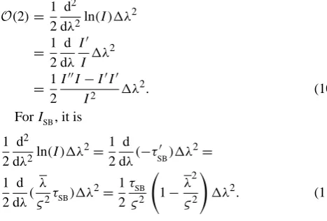
Figure 1a displaysISB(black) fora=0.2 andς=5 pixel, andISBshifted by 1 pixel (blue). Figure 1b shows, in blue, the spectral structure (in terms of OD) caused by the shift, calcu-lated as ln(Ishifted)−ln(I ). In green, the respective structure
resulting from the linearisation in Eq. (3) is shown, i.e., the pseudo-absorberAShift as defined in Eq. (4), scaled by the
applied shift.
ForISB, the shift-spectrum can directly be calculated:
AShift=
I0
SB
ISB = −τ
0 SB=
λ
ς2τSB. (8)
It has its maximum/minimum atλ= ±ς, whereAShiftis ±a
ςe
−12 (compare Fig. 1b). To first order, a spectral shift of
1λ, thus, causes spectral structures (peak-to-peak OD) of
(max(AShift)−min(AShift))×1λ:
O(1)=1.2×a1λ
ς , (9)
i.e., they are proportional to the shift itself, to the depth of the absorption lines, and reciprocal to the width of the absorption lines. In other words, deep narrow absorption lines are most critical for a spectral misalignment. For the sample values (a=0.2,ς=5 and1λ=1), Eq. (9) yields a peak-to-peak OD of 5 %, in agreement with Fig. 1.
It can be seen thatAShiftreproduces well the spectral
struc-tures caused by the shift. The remaining errors, i.e., the dif-ference of the curves in Fig. 1b, are caused by the neglect of higher orders in Eq. (3). The second order term of the Taylor expansion is
O(2)= 1
2 d2
dλ2ln(I )1λ
2
= 1
2 d dλ
I0
I 1λ
2
= 1
2
I00I−I0I0
I2 1λ
2. (10)
ForISB, it is 1
2 d2
dλ2ln(I )1λ
2=1
2 d dλ(−τ
0 SB)1λ
2=
1 2
d dλ(
λ
ς2τSB)1λ
2=1
2
τSB
ς2 1−
λ2
ς2
!
1λ2. (11)
This function is maximum at λ=0 and minimum at
λ= ±
√
3ς. Thus, (Eq. 5), the peak-to-peak distance is
1 2
a
ς2(1+2e
−32)1λ2. The second-order peak-to-peak effects
of a spectral shift are thus
O(2)=0.7×a1λ
2
ς2 . (12)
For the example shown in Fig. 1, this is≈0.6 %, i.e., about one order of magnitude lower than the first-order term ac-counted for byAShift. These orders of magnitudes as derived
for a general absorption band (Eqs. 9 and 12) also proved to be meaningful for complex spectra (see Sect. 4).
The third order term is proportional to1λ3
ς3 , i.e., negligible
for typical shifts (see Sect. 2).
3.2 Spectral stretch
In addition to a spectral shift, the wavelength-pixel alloca-tions might also be linearly transformed by a factorq, i.e., stretched (q >1) or squeezed (q <1) (below we use the generic term “stretch” in a general meaning for bothq >1
andq <1). Here we define the stretchq with respect to the
central wavelength of the fitting windowλ0as:
λ0=q(λ−λ0)+λ0+1λ. (13)
By this definition of the stretch-parameterq, the stretch does not affect the central wavelength of the fitting window, i.e., overall, it does not introduce an additional shift. However, locally, such a stretch is equivalent to a (wavelength depen-dent) shift: at a given wavelength, the spectral displacement
Dcan be expressed as
D:=λ0−λ=q(λ−λ0)+λ0+1λ−λ
=(q−1)(λ−λ0)+1λ, (14)
i.e., locally, a shift of(q−1)(λ−λ0)is added to the
over-all shift1λ. Similarly to1λ, this additional shift causes, in first order, spectral structures ofAShift(λ−λ0)(q−1). Thus,
a spectral stretch can be accounted for by adding the pseudo-absorber (“stretch-spectrum”)
AStretch:=AShift(λ−λ0) (15)
to the linear equation system. The respective fit coefficient is
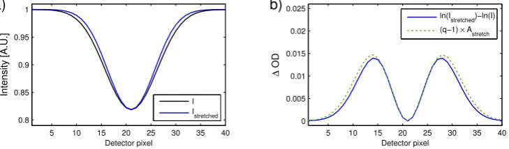
(q−1). Figure 2 shows the effects of a spectral stretch and the stretch spectrum analogously to Fig. 1.
In principle, also higher orders of spectral misalignments (quadratic terms, etc.) could be considered as well in an analogous way, i.e., by defining the pseudo-absorber ofnth order asAn:=AShift(λ−λ0)n. Here, we focus on the effects
of shift (=bA0) and stretch (b=A1).
As a stretch can be regarded as wavelength dependent shift, the errors of the linearisation can be evaluated similar to Sect. 3.1 according to the maximum pixel displacement caused by the stretch.
3.3 Pseudo-absorbers forI0
The shift-spectrum was defined in Eq. (4) based on a Taylor expansion of a shifted radianceI. Here, we define a similar shift-spectrum based onI0:
BShift:=
I00
I0
5 10 15 20 25 30 35 40 0.8
0.85 0.9 0.95 1
Intensity [A.U.]
Detector pixel
a)
I I
shifted
5 10 15 20 25 30 35 40
−0.03 −0.02 −0.01 0 0.01 0.02 0.03
∆
OD
Detector pixel
b)
ln(I shifted)−ln(I)
∆λ× A shift
Fig. 1. Illustration of the effect of a spectral shift ofI. (a) Original (black) and shifted (blue) IntensityIin artificial units, showing a single absorption line according to Eq. (7), with an optical depth ofa=0.2 and a widthς of 5 pixel, for a shift of1λ=1 pixel. (b) Actual difference of the true and shifted OD (blue), compared to the linear approximation, i.e., the pseudo-absorberAShift as defined in Eq. (4),
scaled by the applied shift of 1 pixel (green).
5 10 15 20 25 30 35 40
0.8 0.85 0.9 0.95 1
Intensity [A.U.]
Detector pixel a)
I Istretched
5 10 15 20 25 30 35 40
0 0.005 0.01 0.015 0.02 0.025
∆
OD
Detector pixel b)
ln(I stretched)−ln(I)
(q−1) × A
stretch
Fig. 2. Illustration of the effect of a spectral stretch ofI. (a) Original (black) and stretched (blue) IntensityI in artificial units, showing a single absorption line according to Eq. (7), with an optical depth ofa=0.2 and a widthςof 5 pixel, for a stretch ofq=1.1. (b) Actual difference of the true and stretched OD (blue), compared to the linear approximation, i.e., the pseudo-absorberAStretchas defined in Eq. (15),
scaled by the applied stretchq−1 (green).
The respective stretch-spectrum is defined analogously to Eq. (15):
BStretch:=BShift(λ−λ0). (17)
Deriving the pseudo-absorbers from I0 instead of I may
seem illogical, asI0is spectrally calibrated against a
high-resolution, well-calibrated solar reference and, thus, not subject to further shifts. But if the difference between
BShift/Stretch andAShift/Stretch is negligible, which is the case
if the spectral structures of bothI andI0are dominated by
the strong Fraunhofer lines and the OD of atmospheric ab-sorbersτ is low, this approach has high practical relevance, as it allows one to create a complete, consistent set of refer-ences just based onI0, which can be applied to a sequence
(e.g., one satellite orbit) of radiance measurements. In con-trast, the exact calculation of the pseudo-absorbers based on
I would imply the calculation of the derivative ofIfor each measured spectrum, before the linear fit can be performed.
Both approaches are investigated in the next section for concrete examples, and the applicability of BShift/Stretch
in-stead ofAShift/Stretchis discussed further in Sect. 5.2.
4 Applications
In this section, we analyse the accuracy and performance of the proposed implementation of spectral shift and stretch in the DOAS analysis by pseudo-absorbers, in comparison to the “classical” non-linear DOAS.
In Sect. 4.1, a standard DOAS application, i.e., the fit of NO2 in the blue spectral range, is performed on synthetic
spectra, which allows us to compare the fit results to the a-priori “truth”. In Sect. 4.2, the linearisation is applied to actual satellite measurements for the retrievals of NO2 and
BrO.
4.1 Synthetic spectra
4.1.1 Setup
We consider a detector with a spectral resolution of 0.55 nm FWHM and a spectral sampling of 0.2 nm, as for TROPOMI in the blue spectral range (Veefkind et al., 2012). Starting with a high-resolution solar irradiation spectrum (Chance and Kurucz, 2010),I0 is determined in detector resolution
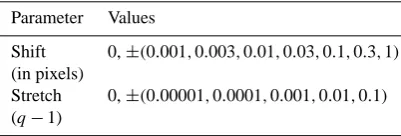
Table 1. Variations of shift and stretch applied to the synthetic spec-tra.
Parameter Values
Shift 0,±(0.001,0.003,0.01,0.03,0.1,0.3,1)
(in pixels)
Stretch 0,±(0.00001,0.0001,0.001,0.01,0.1)
(q−1)
optical depths (peak-to-peak) of 5 % and 1 %, respectively, plus a broad-band absorption. Note that the dependency of the NO2fit bias on shift and stretch, as investigated below, is
not affected by this choice of the a-priori NO2SCD.
I is then manipulated by a variety of spectral displace-ments. Table 1 lists the applied shift and stretch parameters. The fit accuracy is analysed for “ideal” spectra, as well as for spectra where a Gaussian random noise with a standard deviation of 0.015 % of the maximum radiance is added to
I. This noise level corresponds to residues of about 0.1 % peak-to-peak.
The pseudo-absorbers AShift andAStretch are determined
fromI according to Eqs. (4) and (15), andBShiftandBStretch
fromI0according to Eqs. (16) and (17), respectively. Note
that the calculation of the discrete derivativesI0 or I00 has to be done properly, as a simple difference quotient was found to be not accurate enough. This aspect is discussed in Appendix B.
Finally, the shifted and stretched radiances are analysed by linear (with and without the proposed pseudo-absorbers) and non-linear DOAS at 430–450 nm. For this, the commercial software MATLAB, as well as DOASIS (Kraus, 2005), have been used.
4.1.2 Results
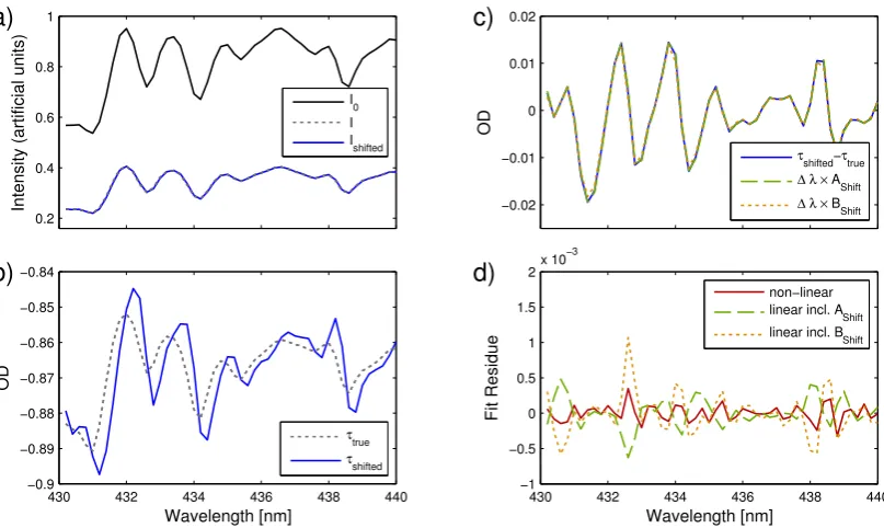
Figure 3 illustrates the effect of the shift and the accuracy of the fit exemplarily for a shift of1λ=0.02 nm, i.e., a tenth of a pixel. The figure displays only half of the fitting window to zoom in the small horizontal displacements.
Figure 3a displaysI0 (black) and the original (grey) and
shifted (blue) radiancesI andIshifted, which can be hardly
discriminated. In Fig. 3b, the respective OD is shown forI
(grey, revealing the combined structures caused by the ap-plied Ring effect and NO2absorption), andIshifted(blue,
re-vealing additional spectral structures due to the shift1λ). In Fig. 3c, the difference of both OD (“true” and “shifted”) from Fig. 3b are displayed in blue, analogously to the sim-ple examsim-ple shown in Fig. 1b, showing spectral structures of about 3.5 % peak-to-peak caused by the spectral mismatch. Note that this structure is very similar to the fit residue of the linear fit without shift- and stretch-spectra (not shown), but not identical, as the fit tries to “explain” part of the shift struc-tures by the considered (pseudo-) absorbers Ring and NO2.
The shift spectraAShiftandBShift, as defined in Eqs. (4) and
(16), scaled by the applied shift, are shown in green/orange, respectively. They both reproduce well the spectral structures caused by the spectral misalignment.
Figure 3d displays the residue of the linear fit including
AShift andAStretch as pseudo-absorbers in green, andBShift
andBStretchin orange. The remaining residue is about 0.11 %
(A) and 0.15 % (B) peak-to-peak, i.e., more than one order of magnitude lower than for the simple linear fit. Note that the residue for the non-linear fit, shown in red, depends on the settings of the Levenberg-Marquardt-Algorithm, in particu-lar on the allowed number of iterations and the predefined termination criteria.
If we estimate the shift effects from Eqs. (9) and (12), we expect (fora≈0.4,ς≈0.3 nm, and1λ=0.02 nm) spectral structures of the order of 3.2 %, in agreement with Fig. 3c, and unresolved residues of about 0.12 %, in good agreement with Fig. 3d. Therefore, the estimates derived for a single band can also be used to estimate the order of magnitude for a complex multi-band spectrum.
In Fig. 4, the fitted shift and stretch parameters are com-pared to the actually applied values. Note that for the linear fit (green), the shift and stretch parameters are simply the fit coefficients for the pseudo-absorbersAShift andAStretch,
i.e.,1λandq−1, respectively, whileI is not changed. In contrast, for the non-linear fit (red), a real shift/stretch is per-formed toI in each iteration step. It can be seen that both fits actually reproduce the applied shifts/stretches with high accuracy. For the non-linear and linear fit, relative deviations between fitted and true shift1λare less than 0.4 % and 3 %, respectively, for displacements<0.03 nm. For a linear fit in-cludingBShift(not shown), the relative deviations are slightly
higher (up to 13 %).
Now we investigate the resulting SCDs for the variety of shifts and stretches listed in Table 1. For each shift/stretch combination, we define the “maximum displacement” as the maximum of all detector pixel displacementsDwithin the fit window, in order to have a single abscissa. For instance, for a shift of 0.1 pixel, i.e., 0.02 nm, and a stretch of 1.0001, the spectral displacement, according to Eq. (14), is maximum at the right edge of the fitting window, where it is(q−1)(λ−
λ0)+1λ=0.021 nm.
Figure 5a shows the resulting fit residues for all combi-nations of shift and stretch, up to a maximum displacement of 0.03 nm, on a log-log-scale. The straight lines indicate the expected first (purple) and second (green) order estimate ac-cording to Eqs. (9) and (12) fora=0.4 andς=0.3 nm. The absolute deviations of the fitted NO2SCDs from the true
(a-priori) value are shown in Fig. 5b. In addition, values for a shift of 0.002 nm are listed in Table 2.
Purple dots show the results for the simple linear fit ignor-ing shift and stretch, revealignor-ing residues accordignor-ing to the first order estimate. For a displacement of 0.002 nm (i.e., 1 % of a pixel), residues are 0.33 %. The respective NO2SCDs are
0.2 0.4 0.6 0.8 1
Intensity (artificial units)
a)
I0
I Ishifted
430 432 434 436 438 440
−0.9 −0.89 −0.88 −0.87 −0.86 −0.85 −0.84
OD
Wavelength [nm]
b)
τ true τ
shifted
−0.02 −0.01 0 0.01 0.02
OD
c)
τ shifted−τtrue ∆λ× A
Shift ∆λ× BShift
430 432 434 436 438 440
−1 −0.5 0 0.5 1 1.5
2x 10 −3
Wavelength [nm]
Fit Residue
d)
non−linear linear incl. AShift linear incl. BShift
Fig. 3. Illustration of the linear and non-linear DOAS fits for a simple synthetic spectrumIincluding the Ring effect and NO2absorption. (a) IntensitiesI0,IandIshifted by 0.02 nm. (b) OD (lnII0) for the original and shifted Intensities. (c) Difference of the OD from shifted
and original Intensities (blue), and the “shift-spectrum” as defined in Eqs. (4) and (16), scaled by the applied shift of 0.02 nm (green/orange). (d) Fit residues for the non-linear fit (red) and the linear fit with shift and stretch pseudo-absorbers included (green/orange).
−1 −0.1 −0.01 0 0.01 0.1 1 −1
−0.1 −0.01 −0.001 0 0.001 0.01 0.1 1
Shift true [pixel]
Shift
fit
[pixel]
a)
non−linear linear
0.99 0.999 1 1.001 1.01 0.99
0.999 0.9999 0.99999 1 1.00001 1.0001 1.001 1.01
Stretch true
Stretch
fit
b)
Fig. 4. Comparison of the fitted and the true shift (left panel, for stretch≡1) and stretch (right panel, for shift≡0) for the non-linear (red) and the linear fit includingAShift andAStretch (green). The applied shifts and stretches are listed in Table 1. The grey line shows 1 : 1
0.0001 0.001 0.01
Residue
10−7 10−6 10−5 10−4 10−3 10−2 10−1
a)
linear lin. incl. Ashift/stretch
lin. incl. Bshift/stretch
non−linear
0.0001 0.001 0.01 Maximum displacement [nm]
1011 1012 1013 1014 1015 1016
NO
2
Fit Bias
[molec/cm
2 ]
b)
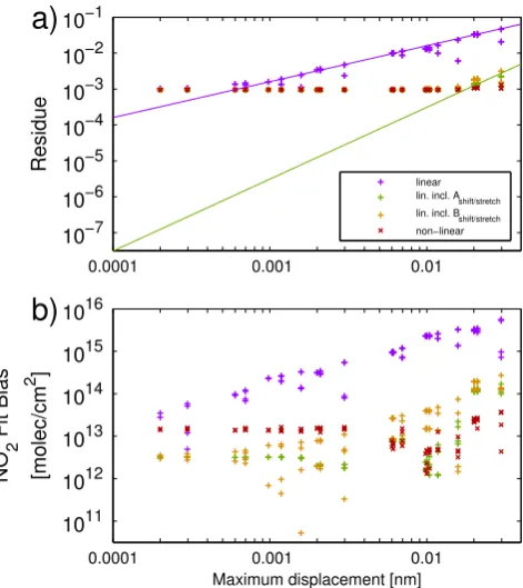
Fig. 5. Dependency of the peak-to-peak fit residue (a) and the abso-lute NO2bias (b) on the maximum spectral displacement caused
by the combined shifts and stretches applied, for the non-linear and various linear fits, on a log-log-scale. The purple and green lines indicate the estimated first and second order effects of a spec-tral displacement, according to Eqs. (9) and (12), fora=0.4 and
ς=0.3 nm.
et al., 2004). Compared to this, the fit results are signifi-cantly improved if shift and stretch are included as pseudo-absorbers to the linear fit (green): both the residue and the NO2bias are generally reduced by more than two orders of
magnitude. At a displacement of 0.002 nm, the residue and NO2 bias are now only about 10−5 and 1012molec cm−2,
respectively, which is negligible, and quite close to the re-sults of the non-linear fit. For pseudo-absorbers derived from I0 (orange), the results are slightly worse (5×10⁻⁵
residue and 5×10¹²molec cm−2bias at 0.002 nm), but still far better than those of a linear fit without pseudo-absorbers. For smaller displacements, the bias decreases approximately quadratically (according to Eq. 12) forA, as expected (as the quadratic term is neglected in Eq. 3). ForB, the decrease is slower (≈linear) due to the additional approximation, i.e., the neglect of atmospheric trace gas absorptions in the calcu-lation of the pseudo-absorbers (compare Eq. 18).
Figure 6 shows the respective fit results averaged for 300 spectra exposed to additional Gaussian noise. Table 2 lists the respective means and standard deviations for a shift of 0.002 nm.
0.0001 0.001 0.01
Residue
10−7 10−6 10−5 10−4 10−3 10−2 10−1
a)
linear lin. incl. Ashift/stretch lin. incl. Bshift/stretch non−linear
0.0001 0.001 0.01 Maximum displacement [nm]
1011 1012 1013 1014 1015 1016
NO
2
Fit Bias
[molec/cm
2 ]
b)
Fig. 6. As Fig. 5 for synthetic radiances with additional Gaussian noise of 0.015 %.
The noise truncates the fit residues (peak-to-peak) of all fits to&0.1 %. Still, the linear fit without shift/stretch per-forms poorly, while the other methods (linear with pseudo-absorbers and non-linear) show lower residues by a factor of about 3 for the typical shifts of 0.002 nm for passive DOAS-applications.
The bias is quite low on average for all fits except the sim-ple linear case. But the standard deviation of the bias caused by the noise is about 1.6×10¹⁴molec cm−2 for a shift of 0.002 nm.
For the noisy radiances, the non-linear fit shows neither lower residues nor lower NO2biasses compared to the linear
fit with pseudo-absorbers. Thus, for practical applications, noise levels of>0.015 % and shifts<0.002 nm, there is no benefit from the non-linear fit at all, and the pseudo-absorbers can be derived fromI0instead ofI, at least for the analysis
of NO2(see also Sect. 4.2 and Sect. 5).
4.1.3 Computation time
Table 2. Fit residues and NO2bias for a shift of 0.002 nm. For the spectra affected to noise, the mean and standard deviation of 300 random spectra is given. All numbers are given with 2 digits, but in fixpoint notation so that the different orders of magnitude are directly visible. The last two fits (5. and 6.) refer to different methods for the calculation of the discrete derivative (see Appendix B) .
Peak-to-peak residue [% OD] NO2bias [1014molec cm−2] w/o noise with noise w/o noise with noise
1. Non-linear 0.00076 (0.095± 0.015) 0.0038 (0.2±1.6) 2. Linear 0.33 (0.34 ± 0.026) 3.2 (3.2±1.6)
3. Linear includingAShift/Stretch 0.0011 (0.095± 0.015) 0.012 (0.0±1.6)
4. Linear includingBShift/Stretch 0.0045 (0.095± 0.015) 0.045 (0.1±1.6) 5. As 3., derivative Eq. (B2) 0.027 (0.10 ± 0.017) 0.48 (0.5±1.7)
6. As 3., derivative Eq. (B3) 0.010 (0.095± 0.015) 0.082 (0.1±1.6)
Table 3. Computation times for linear and non-linear fits from MATLAB and DOASIS in seconds per fit.
Linear fit Non-linear fit
MATLAB 4×10⁻⁵ 5×10⁻² DOASIS 4×10⁻⁴ 4×10⁻³
The computation times for a single fit (without noise) are compared in Table 3. For the spectra affected by Gaus-sian noise, computation times are about 2 to 3 times higher. The non-linear fit is faster by a factor of 10 for the DOA-SIS implementation compared to MATLAB, as could be ex-pected, since DOASIS is optimised for this method, and the mathematical operations are processed by pre-compiled, ex-ecutable code, while MATLAB is a script language. But in-terestingly, for the linear fit, MATLAB performs better than DOASIS; this is probably due to the fact that MATLAB is op-timised for linear matrix operations, while DOASIS does not directly provide the option of a linear fit; instead, the fitted parameters can only be fixed (i.e., the shift can be set to 0). Though we can not comprehend the implementation details of DOASIS, we consider this to be the reason that DOASIS is slower for the “linear” fit compared to MATLAB. We con-clude that DOASIS yields realistic numbers (4×10⁻³s per fit) for the computation time of the non-linear fit, while for the linear fit, the results from MATLAB gives an upper limit of what can be achieved for linear algorithms (4×10⁻⁵s per fit). Therefore, the linear fit is at least faster by two orders of magnitude. Further acceleration of the linear fit can possibly be gained using optimised code on GPUs (Graphic Processor Units), which are particularly suited for linear operations.
If we apply these numbers to one orbit of TROPOMI with about one million spectra (P. Veefkind, personal communi-cation), the computation time would be about 4000 s (>one hour) for the non-linear fit, but only 40 s for the linear fit, without consideration of input/output operations.
4.2 Satellite measurements
In addition to the case study for synthetic spectra, we applied the linearisation scheme also to real satellite measurements for the trace gases NO2(Sect. 4.2.1) and BrO (Sect. 4.2.2),
and compared the results to the routine retrievals at Max-Planck-Institute for Chemistry (MPI-C) Mainz. Both MPI-C retrievals are based on a non-linear Levenberg-Marquardt minimisation algorithm. Spectral shifts, but no stretches, are considered in the routine retrievals, as well as below.
We considered three different linear fit set-ups: 1. a sim-ple linear fit ignoring shift, 2. a linear fit including the shift-spectrumAShiftand 3. a linear fit including the shift-spectrum
BShift, and compared the residues and SCDs to the non-linear
fit. The resulting SCD bias is set in relation to the respective detection limit, which is determined according to Eq. (8.41) in Platt and Stutz (2008). However, we would like to point out that spatio-temporal means of satellite observations can reveal clear patterns far below the detection limit for single measurements, as statistical noise cancels out. Thus, the tol-erable systematic bias is usually lower (about 1/10) than the detection limit for an individual measurement.
For both NO2and BrO, the shift along the orbit has been
found to be>0.01 nm (see Tables 4 and 5). This overall shift can mostly, but not completely, be explained by the Doppler effect (see Sect. 2.2.3). As this overall shift is quite large, but consistent along the orbit, it could be a-priori accounted for by shifting all radiancesI by this overall shift before per-forming the fit. However, if undersampling effects can be ne-glected, this is mathematically equivalent to shifting the set of references (I0, cross-sections and pseudo-absorbers)
to-wardsI instead. Therefore,I0and all
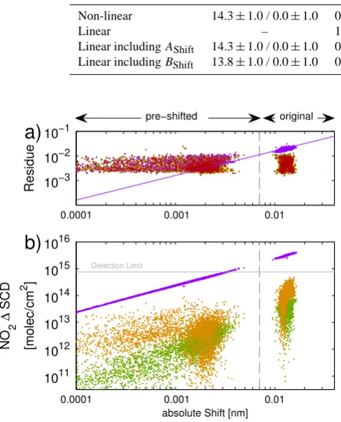
Table 4. Comparison of the results of the non-linear and the different linear fits applied to SCIAMACHY measurements on 1 June 2006. Spectral shift, fit residues, and NO2SCD bias are displayed as mean±standard deviation, first for the original, then (separated by “/”) for
the pre-shifted set of references.
Fit Shift Peak-to-peak residue NO21SCD
[10−3nm] [% OD] [1014molec cm−2] Non-linear 14.3±1.0 / 0.0±1.0 0.20±0.04 / 0.20±0.04 ≡0 (by definition) Linear – 1.95±0.15 / 0.24±0.06 34.32±2.67 /−0.06±2.45 Linear includingAShift 14.3±1.0 / 0.0±1.0 0.21±0.04 / 0.20±0.04 −0.62±0.10 /−0.00±0.01
Linear includingBShift 13.8±1.0 / 0.0±1.0 0.21±0.04 / 0.20±0.04 0.91±0.26 / 0.02±0.02
0.0001 0.001 0.01
10−3
10−2
10−1
Residue
a)
0.0001 0.001 0.01 Detection Limit
absolute Shift [nm]
1011
1012
1013
1014
1015
1016
NO
2
∆
SCD
[molec/cm
2 ]
b)
pre−shifted original
Fig. 7. Dependency of the peak-to-peak fit residues (a) and the ab-solute NO2SCD bias with respect to the non-linear fit (b) on the
absolute spectral shift (as found by the non-linear fit). Colours as in Fig. 5. The purple line corresponds to Eq. (9) fora=0.4 and
ς=0.3 nm. Results from the original (shift>0.007 nm) and the pre-shifted set of references (shift<0.007 nm) are combined.
4.2.1 Retrieval of Nitrogen dioxide – NO2
The routine MPI-C retrieval of NO2from SCIAMACHY is
described in Beirle and Wagner (2012). Here we analyse the first orbit of 1 June 2006.
Figure 7 shows (a) the resulting residues (peak-to-peak) and (b) NO2SCD deviations to the non-linear fit, in
depen-dency of the fitted spectral shift (from the non-linear fit), sim-ilar as Figs. 5 and 6. The mean shifts, residues, and SCD bi-asses are listed in Table 4. Note that Fig. 7 shows absolute values both on x and y axis, as the scales are logarithmic, but the means listed in Table 4 are calculated for the signed val-ues and can thus be far lower if positive and negative numbers cancel each other out.
For the original set of references, a mean shift of
≈0.014 nm is found for the complete orbit. The fitted shifts
using the pre-shifted set of references are far lower. Com-bined, both fits reveal a consistent dependency of residues and SCD biasses over a large variety of spectral shifts.
Generally, the results are quite similar to the fit of syn-thetic spectra (compare Figs. 5 and 6). For large shifts (original set of references), the residues of the simple lin-ear fit (purple) show the expected linlin-ear dependency on the shift, even matching quantitatively the estimation according to Eq. (9). The fit residues for the other fits (linear with pseudo-absorbersA(green)/B(orange) and non-linear (red)) are similar to each other and show no dependency on the shift, i.e., they are dominated by spectral noise and potential systematic spectral structures of about 0.2 % peak-to-peak, which is slightly higher than the noise applied for the syn-thetic fits. The difference of residues compared to the non-linear fit (not shown), i.e., the additional residue due to the linearisation, decreases further towards low shifts, following Eq. (12) and shown as green line in Fig. 5.
The bias in NO2 SCD for the simple linear fit shows a
clear linear dependency on the spectral shift, as for the syn-thetic case study. It is, on average, 3.4×10¹⁵molec cm−2for the original set of references, which is significantly higher than the NO2detection limit, and would not be tolerable for
satellite retrievals of NO2. For the pre-shifted set of
refer-ences, positive and negative shifts cancel each other, lead-ing to a low bias on average (0.06 ×10¹⁴molec cm−2 ). But the SCD deviations for individual pixels can still reach 1×10¹⁵molec cm−2.
The linear fit including AShift performs very well.
Devi-ations from the non-linear fit are only −0.62 and −0.004
×1014molec cm−2 for the original/pre-shifted set of refer-ences, respectively. UsingBShiftinstead ofAShiftslightly
de-grades the agreement (also for the fitted shift), but still, the mean bias would be acceptable even for the original set of references without pre-shift.
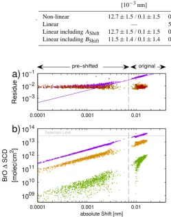
Table 5. Comparison of the results of the non-linear and the different linear fits applied to GOME-2 measurements on 12 April 2009. Spectral shift, fit residues, and BrO SCD bias are displayed as mean±standard deviation, first for the original, then (separated by “/”) for the pre-shifted set of references.
.
Fit Shift Peak-to-peak residue BrO1SCD [10−3nm] [% OD] [1012molec cm−2] Non-linear 12.7±1.5 / 0.1±1.5 0.82±0.22 / 0.82±0.22 ≡0 (by definition) Linear — 5.93±0.75 / 1.05±0.34 −32.31±4.01 / 0.23±3.89 Linear includingAShift 12.7±1.5 / 0.1±1.5 0.87±0.22 / 0.82±0.22 −0.52±0.20 / 0.00±0.02
Linear includingBShift 11.5±1.4 / 0.1±1.4 0.90±0.22 / 0.82±0.22 9.69±1.78 /−0.02±0.93
0.0001 0.001 0.01
10−3
10−2
10−1
Residue
a)
0.0001 0.001 0.01
Detection Limit
absolute Shift [nm]
1009
1010
1011
1012
1013
1014
BrO
∆
SCD
[molec/cm
2 ]
b)
pre−shifted original
Fig. 8. Dependency of the fit residues (a) and the absolute BrO SCD bias with respect to the non-linear fit (b) on the absolute spectral shift. Colours as in Fig. 5. The purple line corresponds to Eq. (9) fora=0.7 andς=0.2 nm. Results from the original and the pre-shifted set of references are combined.
be interpreted as kind of overall error or detection limit, but nicely illustrate how close the linear results can reproduce the non-linear fit.
4.2.2 Retrieval of Bromine monoxide – BrO
The routine MPI-C retrieval of BrO from GOME-2 is de-scribed in Sihler et al. (2012). Here we analyse an orbit of 12 April 2009 for the Northern Hemisphere, where enhanced tropospheric BrO was observed in the Beaufort sea (see page 17 of the Supplement of Sihler et al., 2012). Figure 8 shows (a) the resulting residues (peak-to-peak) and (b) BrO SCD deviations to the non-linear fit, analogue to Fig. 7. Table 5 lists the respective orbit means and standard deviations.
The results are similar to those for NO2(Sect. 4.2.1), but
with some differences in detail. The simple linear fit again results in a clear dependency of residues (for shifts above
≈0.005 nm) and BrO biasses on the absolute spectral shift. But the slope of the residue is higher than for NO2due to the
deeper Fraunhofer lines in the fitting window. The purple line in Fig. 8a corresponds to Eq. (9) fora=0.7 andς=0.2 nm. The residues of the other fits again show no dependency on the shift, and are generally higher (about 0.8 % peak-to-peak OD) than for NO2.
The simple linear fit results in a mean bias of−3.2×10¹³ molec cm−2for the original set of references, which would not be tolerable. In contrast, the linear fit including AShift
works very well and yields results very close to those of the non-linear fit. The mean bias of −0.52 ×10¹²molec cm−2 for the original set of references is negligible.
IncludingBShiftyields again lower SCD biasses (1×10¹³
molec cm−2) than the simple linear fit. But the improvement is less distinct than in the case of NO2. This is due to the
fact that the difference ofAShiftandBShiftis determined by
the derivative of the OD, which is generally higher for the BrO fit, mainly due to the Ring effect and ozone absorption (see Sect. 5.2). The resulting SCD bias is slightly below the detection limit of BrO, but still high enough to significantly affect spatio-temporal means.
This case study clearly illustrates that the linearisation in-cludingAShift also works for a weak absorber as BrO. The
question whetherBShiftcould be used instead depends on the
accuracy requirements and has to be investigated for each trace gas and fitting window individually. In several cases, the a-priori correction of the Doppler-shift by pre-shifting the set of references will allow the usage ofBShift.
5 Discussion
5.1 Quick assessment of the spectral calibration
Apart from fitting trace gas SCDs, the pseudo-absorbers
AShift/Stretch allow the quick assessment of the spectral
cal-ibration of a given spectrum: the respective fit parameters di-rectly yield the spectral shift1λand stretch(q−1). Thus, for example, the mean spectral shift of satellite measurements can quickly be determined, or the need for accounting for a spectral stretch can be easily evaluated.
5.2 Pseudo-absorbers derived fromI0
As mentioned in Sect. 3.3, calculating the pseudo-absorbers fromI00/I0instead of I0/I has high practical relevance for
satellite retrievals:I00/I0needs to be calculated only once per
reference spectrum, i.e., once per day for satellite measure-ments, thereby providing one consistent set of references for the complete day.
For passive DOAS applications, both I and I0 are
usu-ally dominated by the strong Fraunhofer lines. Thus,BShiftis
generally similar toAShift; they differ by the derivative of the
OD:
BShift−AShift=τ0 (18)
(compare Eq. 1).
Forτ with a peak-to-peak OD ofb, the order of magnitude ofτ0is aboutb/ς. If, in addition, the spectral structures of the OD are dominated by the Ring effect, the peak widthς will be similar to that ofI. Consequently, the relative deviation betweenAShift andBShift is aboutb/a, i.e., the ratio of the
order of magnitude ofτand the depth of the Fraunhofer lines. Note that the impact on the fit results is even less, asBShift
can be scaled by the fit. Therefore, only different patterns of
BShiftcompared toAShiftcan cause an additional SCD bias.
For NO2, the errors induced by BShift/Stretch have been
found to be generally negligible (Figs. 6 and 7). However, this is different for DOAS evaluations for trace gases absorb-ing in the UV, like BrO, due to the higher OD of Ozone and the Ring effect.
If the errors caused by the pseudo-absorbersBcan not be neglected, andAhave to be used, the derivative ofI has to be calculated for each individual measured spectrum. This reduces the acceleration due to the linearisation by about 20 %, if the derivative is calculated according to Eq. (B3) (see Appendix B).
Alternatively, we propose to apply a pre-shift to the set of references (next section), which results in significantly lower remaining shifts and, thus, allows one to useBinstead ofA
for the investigated examples.
5.3 Pre-shifted set-up
For satellite measurements, the spectral shift is dominated by the Doppler-effect of'0.01 nm at 440 nm. For NO2as well
as BrO, the linearisation based on the pseudo-absorbersA
works well (i.e., SCD biasses are negligible) even for such large shifts. However, as the observed shifts are quite consis-tent along the orbit, we propose to correct for the overall shift by pre-shifting the set of references I0, cross-sections and
pseudo-absorbers accordingly (see Sect. 4.2). (The a-priori required overall shift could, for example, be taken from the previous day in routine retrievals of satellite data). The re-maining shifts (relative to this overall shift) are considerably smaller, resulting in far lower SCD biasses due to the lineari-sation, thus, facilitating the use of the pseudo-absorbersB in-stead ofA(see previous section), even for the BrO retrieval.
5.4 Missing pixels
An additional advantage of the proposed implementation of spectral misalignments by pseudo-absorbers derived from
I0 instead ofI is the evaluation of radiance measurements
I containing gaps (e.g., due to dead detector pixels); such gaps are problematic for the non-linear fit, as shiftingI in-volves interpolation and one missing pixel, thus, affects (i.e., removes) its neighbours as well. In contrast, for the linear fit, the dead pixels can just be skipped forI,I0,σ and the
pseudo-absorbers likewise, and the effect of a potential shift is still accounted for appropriately by the pseudo-absorbers.
In the case of gaps inI0, however, these have to be filled in
first (e.g., by fitting another solar reference without gaps plus a polynomial), before the derivativeI00can be calculated.
5.5 Initialization of the non-linear fit
Even if a non-linear DOAS analysis is unavoidable for a given set-up, e.g., due to large shifts or other effects causing nonlinearities, the linear fit could still be applied for the cal-culation of the initial state vector. The subsequent non-linear fit benefits from accurate initial values for SCDs and particu-larly shift and stretch, and will be more robust and faster. For instance, for a shift of 0.002 nm, the non-linear fit becomes 30 % faster if initialised with the linear fit results including shift- and stretch-spectra.
6 Conclusions
Spectral misalignments cause biasses in a DOAS analysis and can generally not be neglected. As a consequence, non-linear minimisation algorithms are applied in state-of-the-art DOAS analyses, which are far slower than linear algorithms. We propose to linearise the effects of spectral shifts by the first-order term of a Taylor expansion and introduce a “shift-spectrum”
AShift:=
I0(λ)
I (λ)
−1 −0.1 −0.01 0 0.01 0.1 1 −1
−0.1 −0.01 −0.001 0 0.001 0.01 0.1 1
Shifttrue [pixel]
Shift
fit
[pixel]
a)
linear non−linear
0.99 0.999 1 1.001 1.01 0.99
0.999 0.9999 0.99999 1 1.00001 1.0001 1.001 1.01
Stretchtrue
Stretch
fit
b)
Fig. A1. As Fig. 4, but for shifts in the absorption cross-section of NO2. The fitted shifts/stretches forAσShiftandAσStretchare off by almost an order of magnitude due to the remaining nonlinearities (see text).
Spectral stretches can be considered as well by a “stretch-spectrum”
AStretch:=AShift(λ−λ0),
as they can be regarded as additional wavelength-dependent shifts.
With these pseudo-absorbers, the DOAS-analysis can be performed linearly, reducing the computational costs by at least 2 orders of magnitude. This is particularly relevant for satellite measurements with high data rates.
The error due to the linearisation, in terms of peak-to-peak OD, is
0.7×a1λ
2
ς2 ,
where a and ς are the band depths and widths of I, re-spectively. For typical shifts about 0.14 nm, this error is about 6×10⁻⁴ for NO2 (a≈0.4, ς ≈0.3 nm), and about
2.4×10⁻³for BrO (a≈0.7, ς≈0.2 nm), thus, significantly lower than the actual noise levels for the investigated re-trievals of NO2and BrO from SCIAMACHY and GOME-2,
respectively. The resulting biasses of SCDs have been found to be negligible.
Full advantage of the linearisation could be gained if the pseudo-absorbers are calculated based onI0 (instead ofI),
as these have to be derived only once per reference spectrum instead of once per measurement:
BShift:=
I00(λ)
I0(λ)
BStretch:=BShift(λ−λ0).
For weak absorbers like NO2, this is generally
applica-ble. For strong absorbers like O3in the BrO or SO2fit, the
pseudo-absorbersAmight have to be calculated for each ra-diance spectrum, reducing the speed of the linear fit by about 20 %.
Alternatively, the applicability ofBcan be achieved if the overall shift betweenI andI0is accounted for by an a-priori
“pre-shift”. For the investigated retrievals of NO2 and BrO
from SCIAMACHY and GOME-2, respectively, the remain-ing shifts are about/0.003 nm, and the SCD biasses result-ing from a linear fit includresult-ingB are negligible even in the case of BrO.
Even if a non-linear fit is unavoidable (for larger shifts or other non-linear effects), the linear fit can still yield a quick assessment of the spectral calibration ofI and an accurate initial state vector for shift and stretch in the non-linear fit.
Appendix A
Spectral misalignments of a cross-section
A cross-section included in a DOAS analysis might be af-fected by an imperfect spectral calibration as well. Note, however, that there is a basic mathematical difference be-tween intensities and sections in Eq. (1), as the cross-sections are scaled by the SCD during the fit.
In general, the spectral structures resulting from a shift in
σ could be estimated by a Taylor expansion ofσ as well:
σ (λ+1λ)=σ (λ)+ d
dλσ (λ)1λ+O(2)
≈σ (λ)+AσShift1λ (A1)
with the pseudo-absorber
AσShift:=σ0= d
dλσ . (A2)
However, the relevant respective structure in OD would be
AσShift×1λ×s. Therefore, the fit coefficientswould appear
Figure 5.3 shows the results for a linear fit includingAσShift
(i.e., ignoring that the problem is not really linear) for the example of a synthetic spectrum with Ring effect (5 % OD) and NO2absorption (5 % OD), where the NO2cross-section
is shifted and stretched. Obviously, the applied shifts and stretches are not reproduced by the linear fit due to the re-maining nonlinearity. The fit accuracy for NO2is not much
better than that of a simple linear fit ignoring shift effects completely.
Fortunately, spectral shifts ofσ do not have a high rele-vance in most DOAS applications, as cross-sections can gen-erally be measured in laboratory with high accuracy. Ad-ditionally, a shift could only significantly affect the DOAS analysis if the respective absorber has a high OD of several percent and narrow absorption lines. Thus, normally, spec-tral shifts of cross-sections can be neglected. But in the case of an analysis where spectral shifts ofσ actually occur for a strong absorber, these shifts have either to be determined (and corrected) independently, or the DOAS analysis has to be performed by a non-linear algorithm.
Appendix B
Discrete derivative
The shift-spectrum involves the first derivative ofI, which has to be calculated numerically. For the comparison of the linear and non-linear fit in Sect. 4, we calculate the derivative of the discrete functionsI andI0by mimicking the
differ-ence quotient according to
y0=y(x+h)−y(x)
h , (B1)
whereyisI orI0, respectively,xis the (integer) pixel
num-ber,his set to 0.0001 pixel, andy(x+h)is derived by cubic spline interpolation ofy.
This approach proves to yield accurate results for the lin-ear fit, particularly for small shifts, but is a rather time-consuming method.
Alternatively, we investigate the fit accuracy for the dis-crete derivatives
y00 = 1
2h(−y−1+y1), (B2)
and
y00 = 1
12h(y−2−8y−1+8y1−y2) (B3)
according to Bronstein and Semendjajew (1981) (Sect. 7.1, Table 7.13 therein), where h is the distance between two
y values. The unit chosen for h (i.e., 1 pixel or the corre-sponding wavelength interval) determines the units of the derivative and the fitted shift, respectively.
Table 2 lists the respective fit residues and SCD bias of the different derivative definitions for a shift of 0.002 nm. Com-pared to the spline-based derivative, both derivatives result in higher residues and SCD bias. However, for the spectra affected by noise, results from the fit using Eq. (B3) are quite close to the spline-based results. Thus, we propose to calcu-late the discrete derivative according to Eq. (B3), which is far faster than the spline-based derivative, and shows far better fit results compared to derivatives based on Eq. (B2).
Strictly speaking, the derivative ofI0would have to be
cal-culated from the high-resolution solar reference, convolved with the instrument spectral response function afterwards. However, here we calculate all derivatives (for AShift and
BShift) on the spectrometer’s grid and resolution (FWHM
0.55 nm). This approximation does not affect our results; the introduced errors are small compared to other effects (e.g., the appropriate discrete derivative method).
Acknowledgements. We thank Julia Remmers, Kornelia Mies (both
MPI-C Mainz), Andreas Richter (University Bremen), and two anonymous reviewers for helpful comments on the manuscript. Oliver Woodford is acknowledged for providing the MATLAB routineexport fig, which significantly simplifies the processing of MATLAB figures.
Edited by: A. J. M. Piters
The service charges for this open access publication have been covered by the Max Planck Society.
References
Beirle, S. and Wagner, T.: Tropospheric vertical column den-sities of NO2 from SCIAMACHY, available at: http://www.
sciamachy.org/products/NO2/NO2tc v1 0 MPI AD.pdf (last ac-cess: 12 March 2013), 2012.
Boersma, K., Eskes, H., and Brinksma, E.: Error analysis for tropo-spheric NO2retrieval from space, J. Geophy. Res., 109, D04311,
doi:10.1029/2003JD003962, 2004.
Bronstein, I. N. and Semendjajew, K. A.: Taschenbuch der Mathe-matik, 20th Edn., Verlag Harri Deutsch, Thun, 1981.
Chance, K.: Analysis of BrO measurements from the Global Ozone Monitoring Experiment, Geophys. Res. Lett., 25, 3335–3338, doi:10.1029/98GL52359, 1998.
Chance, K. and Kurucz, R. L.: An improved high-resolution solar reference spectrum for Earth’s atmosphere measurements in the ultraviolet, visible, and near infrared, J. Quant. Spectrosc. Ra., 111, 1289–1295, doi:10.1016/j.jqsrt.2010.01.036, 2010. Chance, K. V. and Spurr, R. J. D.: Ring effect studies: Rayleigh
scattering, including molecular parameters for rotational Raman scattering, and the Fraunhofer spectrum, Appl. Opt., 36, 5224– 5230, doi:10.1364/AO.36.005224, 1997.
H¨onninger, G., von Friedeburg, C., and Platt, U.: Multi axis dif-ferential optical absorption spectroscopy (MAX-DOAS), Atmos. Chem. Phys., 4, 231–254, doi:10.5194/acp-4-231-2004, 2004. Kraus, S.: DOASIS: A framework design for DOAS, Dissertation,
University of Mannheim, Germany, 2005.
Marquardt, D. W.: An algorithm for least-squares estimation of non-linear parameters, J. Soc. Ind. Appl. Math., 11, 431–441, 1963. Martin, R.: Satellite remote sensing of surface air quality, Atmos.
Environ., 42, 7823–7843, doi:10.1016/j.atmosenv.2008.07.018, 2008.
Noxon, J., Whipple, E., and Hyde, R.: Stratospheric NO2. 1.
Obser-vational Method and Behavior at Mid-Latitude, J. Geophys. Res.-Ocean. Atmos., 84, 5047–5065, doi:10.1029/JC084iC08p05047, 1979.
Platt, U.: Differential optical absorption spectroscopy (DOAS), in: Air Monitoring by Spectroscopic Techniques, Chemical Anal-ysis Series, edited by: Sigrist, M. W., John Wiley, New York, 127 pp., 1994.
Platt, U. and Stutz, J.: Differential Optical Absorption Spec-troscopy, Springer-Verlag, Berlin, Heidelberg, 2008.
Richter, A. and Wagner, T.: The Use of UV, Visible and Near IR Solar Back Scattered Radiation to Determine Trace Gases, in: The Remote Sensing of Tropospheric Composition from Space, edited by: Burrows, J. P., Borrell, P., and Platt, U., Springer, available at: http://www.springerlink.com/content/ x66428846gu0870k/abstract/ (last access: 11 May 2012), Berlin, Heidelberg, 67–121, 2011.
Rozanov, A., K¨uhl, S., Doicu, A., McLinden, C., Puk¸¯ıte, J., Bovens-mann, H., Burrows, J. P., DeutschBovens-mann, T., Dorf, M., Goutail, F., Grunow, K., Hendrick, F., von Hobe, M., Hrechanyy, S., Lichtenberg, G., Pfeilsticker, K., Pommereau, J. P., Van Roozen-dael, M., Stroh, F., and Wagner, T.: BrO vertical distributions from SCIAMACHY limb measurements: comparison of algo-rithms and retrieval results, Atmos. Meas. Tech., 4, 1319–1359, doi:10.5194/amt-4-1319-2011, 2011.
Sihler, H., Platt, U., Beirle, S., Marbach, T., K¨uhl, S., D¨orner, S., Verschaeve, J., Frieß, U., P¨ohler, D., Vogel, L., Sander, R., and Wagner, T.: Tropospheric BrO column densities in the Arctic derived from satellite: retrieval and comparison to ground-based measurements, Atmos. Meas. Tech., 5, 2779– 2807, doi:10.5194/amt-5-2779-2012, 2012.
Slijkhuis, S., von Bargen, A., Thomas, W., and Chance, K.: Calcula-tion of under-sampling correcCalcula-tion spectra for DOAS spectral fit-ting, in: ESAMS99 European Symposium on Atmospheric Mea-surements From Space, Rep. ESA WPP-161, Eur. Space Agency, Noordwijk, The Netherlands, 563–569, 1999.
Solomon, S., Schmeltekopf, A. L., and Sanders, R. W.: On the in-terpretation of zenith sky absorption measurements, J. Geophys. Res., 92, 8311–8319, doi:10.1029/JD092iD07p08311, 1987. Stutz, J. and Platt, U.: Numerical analysis and estimation of the
statistical error of differential optical absorption spectroscopy measurements with least-squares methods, Appl. Opt., 35, 6041– 6053, doi:10.1364/AO.35.006041, 1996.
Vandaele, A. C., Hermans, C., Simon, P. C., Carleer, M., Colin, R., Fally, S., M´erienne, M. F., Jenouvrier, A., and Coquart, B.: Measurements of the NO2 absorption
cross-section from 42 000 cm−1 to 10 000 cm−1 (238–1000 nm) at 220 K and 294 K, J. Quant. Spectrosc. Ra., 59, 171–184, doi:10.1016/S0022-4073(97)00168-4, 1998.
Veefkind, J. P., Aben, I., McMullan, K., Forster, H., de Vries, J., Otter, G., Claas, J., Eskes, H. J., de Haan, J. F., Kleipool, Q., van Weele, M., Hasekamp, O., Hoogeveen, R., Landgraf, J., Snel, R., Tol, P., Ingmann, P., Voors, R., Kruizinga, B., Vink, R., Visser, H., and Levelt, P. F.: TROPOMI on the ESA Sentinel-5 precursor: AGMES mission for global observations of the atmospheric composition for climate, air quality and ozone layer applications, Remote Sens. Environ., 120, 70–83, doi:10.1016/j.rse.2011.09.027, 2012.
Wagner, T., Beirle, S., Deutschmann, T., Eigemeier, E., Franken-berg, C., Grzegorski, M., Liu, C., Marbach, T., Platt, U., and de Vries, M. P.: Monitoring of atmospheric trace gases, clouds, aerosols and surface properties from UV/vis/NIR satellite instru-ments, J. Opt. A-Pure Appl. Op., 10, 104019, doi:10.1088/1464-4258/10/10/104019, 2008.
Wagner, T., Beirle, S., Brauers, T., Deutschmann, T., Frieß, U., Hak, C., Halla, J. D., Heue, K. P., Junkermann, W., Li, X., Platt, U., and Pundt-Gruber, I.: Inversion of tropospheric profiles of aerosol extinction and HCHO and NO2 mixing ratios from
MAX-DOAS observations in Milano during the summer of 2003 and comparison with independent data sets, Atmos. Meas. Tech., 4, 2685–2715, doi:10.5194/amt-4-2685-2011, 2011.