Investigating the long-term evolution of subtropical ozone proﬁles applying ground-based FTIR spectrometry

(1)

www.atmos-meas-tech.net/5/2917/2012/ doi:10.5194/amt-5-2917-2012

Measurement

Techniques

Investigating the long-term evolution of subtropical ozone profiles

applying ground-based FTIR spectrometry

O. E. Garc´ıa1, M. Schneider2,1, A. Redondas1, Y. Gonz´alez1, F. Hase2, T. Blumenstock2, and E. Sep ´ulveda3,1

1_{Iza˜na Atmospheric Research Centre (IARC), Agencia Estatal de Meteorolog´ıa (AEMET), Santa Cruz de Tenerife, Spain} 2_{Institute for Meteorology and Climate Research (IMK-ASF), Karlsruhe Institute of Technology (KIT), Karlsruhe, Germany} 3_{University of La Laguna, La Laguna, Spain}

Correspondence to: O. E. Garc´ıa ([email protected])

Received: 9 February 2012 – Published in Atmos. Meas. Tech. Discuss.: 10 May 2012 Revised: 17 October 2012 – Accepted: 4 November 2012 – Published: 28 November 2012

Abstract. This study investigates the long-term evolution of subtropical ozone profile time series (1999–2010) obtained from ground-based FTIR (Fourier Transform InfraRed) spec-trometry at the Iza˜na Observatory ozone super-site. Different ozone retrieval strategies are examined, analysing the influ-ence of an additional temperature retrieval and different con-straints. The theoretical assessment reveals that the FTIR sys-tem is able to resolve four independent ozone layers with a precision of better than 6 % in the troposphere and of better than 3 % in the lower, middle and upper stratosphere. This total error includes the smoothing error, which dominates the random error budget. Furthermore, we estimate that the measurement noise as well as uncertainties in the applied at-mospheric temperature profiles and instrumental line shape are leading error sources. We show that a simultaneous tem-perature retrieval can significantly reduce the total random errors and that a regular determination of the instrumental line shape is important for producing a consistent long-term dataset. These theoretical precision estimates are empirically confirmed by daily intercomparisons with Electro Chemical Cell (ECC) sonde profiles. In order to empirically document the long-term stability of the FTIR ozone profile data we compare the linear trends and seasonal cycles as obtained from the FTIR and ECC time series. Concerning seasonality, in winter both techniques observe stratospheric ozone pro-files that are typical middle latitude propro-files (low tropopause, low ozone maximum concentrations) and in summer/autumn profiles that are typical tropical profiles (high tropopause, high maximum concentrations). The linear trends estimated from the FTIR and the ECC datasets agree within their er-ror bars. For the FTIR time series, we observe a significant

negative trend in the upper troposphere/lower stratosphere of about−0.2 % yr−1and a significant positive trend in the middle and upper stratosphere of about +0.3 % yr−1 and

+0.4 % yr−1, respectively. Identifying such small trends is a difficult task for any measurement technique. In this context, super-sites applying different techniques are very important for the detection of reliable ozone trends.

1 Introduction

(2)

also (WMO, 2011). In order to verify or decline the different climate model simulations consistent long-term observations of the vertical distribution of ozone are required. Since the expected signals are rather small (e.g., expected trends from

−3 % to +1 % per decade between 1960 and 2100, Hegglin and Shepherd, 2009; Li et al., 2009), only high precision ob-servations are useful.

Within the NDACC (Network for the Detection of At-mospheric Composition Change, e.g., Kurylo and Zander, 2000) high resolution solar absorption infrared spectra have been measured by ground-based FTIR (Fourier Transform InfraRed) spectrometers for up to two decades at globally distributed sites. It has been shown that these measurements can provide very high quality ozone total column amounts (Schneider and Hase, 2008; Schneider et al., 2008a; Viatte et al., 2011) and profiles (Schneider et al., 2008b). Due to its long-term characteristic and its high precision, the FTIR data are very interesting for trend studies. Vigouroux et al. (2008) (updated in WMO, 2011) estimated ozone trends at several European NDACC FTIR sites. In this work, we ex-amine in detail the FTIR error sources and discuss how they can affect the estimated ozone trends. We present three dif-ferent FTIR ozone profile retrieval setups, including the setup applied by Vigouroux et al. (2008), and discuss their reliabil-ity for providing correct ozone trend estimates. This study is performed for the ozone super-site Iza˜na Observatory, where since 1999 the FTIR measurements have been performed co-incidently to several other high quality atmospheric ozone measurement techniques (e.g., Brewer spectrometer, Electro Chemical Cell, ECC, sondes, photometric in situ surface).

The Iza˜na Observatory and its Ozone Program is described in Sect. 2. In Sect. 3, we present the three different FTIR re-trieval setups, perform detailed theoretical error estimations and discuss the error sources that can affect trend estima-tions. In Sect. 4, we briefly discuss the quality of the ECC sonde data and in Sect. 5 we show a day-to-day compari-son between the three different FTIR datasets and the ECC dataset. In Sect. 6, we present the ozone seasonality and the trends obtained at different altitudes from the different FTIR datasets and discuss their consistency to the values obtained for the ECC dataset. Finally, the main results are summarised in Sect. 7.

2 The Iza ˜na Observatory and its ozone program

The Iza˜na Observatory (28.3◦_{N, 16.5}◦_{W) belongs to the}

Spanish Meteorological Agency (AEMET). It is a subtrop-ical high mountain observatory, located at 2.37 km altitude on Tenerife Island, and typically above a temperature inver-sion layer which acts as a natural barrier for local pollution. Hence, it offers excellent conditions for the remote-sensing of the upper atmosphere.

Since many years the Iza˜na Observatory has been a WMO/GAW (World Meteorological Organisation/Global

Atmospheric Watch) station and an NDACC site, moni-toring a large variety of atmospheric constituents, among them, ozone total column amounts and ozone profiles. Dif-ferent ozone measuring techniques are applied: Brewer spec-trometer, FTIR specspec-trometer, Differential Optical Absorption Spectroscopy (DOAS), in situ ultraviolet photometric analy-sers, and ECC sondes. In this study, we focus on ozone pro-files and in the following two subsections we briefly describe the techniques that can measure ozone concentrations at dif-ferent altitudes above the Iza˜na Observatory.

2.1 FTIR program

Ground-based FTIR systems measure solar absorption spec-tra applying a high resolution Fourier Transform spectrom-eter. The FTIR activities at Iza˜na started in 1999 when, in the framework of a collaboration between AEMET and KIT (Karlsruhe Institute of Technology, Germany), a Bruker IFS 120M was installed at the Observatory. In January 2005 KIT scientists substituted this spectrometer by a Bruker IFS 120/5HR, which is one of the best performing FTIR spectrometers commercially available. During March and April 2005 both instruments measured side-by-side, which allows for documenting the consistency of both FTIRs.

Since 1999, the Iza˜na experiment provides data to the NDACC network. Currently there are about 25 ground-based FTIR NDACC experiments. For NDACC, the solar absorp-tion spectra are measured in the mid-infrared spectral region (740 and 4250 cm−1, corresponding to 13.5 and 2.4 µm), which is covered by six individual measurements apply-ing different filters in order to achieve an optimal signal-to-noise ratio. In this spectral region, the FTIR spectra are recorded using a potassium bromide (KBr) beamsplitter, whereby two liquid nitrogen-cooled detectors are applied: a mercury cadmium telluride (MCT) for wavenumbers below 1850 cm−1 and an indium antimonide photododiode (InSb) for higher wavenumbers. For operational ozone measure-ments the FTIR spectra covering the 1000 cm−1 region were measured with an aperture of 1.5 mm, which corre-sponds to a field-of-view of only 0.2◦. Therefore, the FTIR instrument only analyses sunlight coming from the centre of the solar disc (diameter of 0.5◦). In order to increase the signal-to-noise ratio several scans, with a high spectral res-olution of 0.005 cm−1 (maximum Optical Path Difference, OPDmax of 180 cm), are co-added (8 for the ozone

mea-surements). Thereby, the measurement of one spectrum takes about 10 min. At Iza˜na the FTIR spectra typically are mea-sured on two or three days per week.

2.2 ECC and in situ surface program

(3)

Fig. 1. Spectral microwindow applied for ozone retrievals.

Observatory: from Santa Cruz de Tenerife (35 km northeast of the Observatory) and since October 2006 from G¨u´ımar (15 km east of the Observatory). Smit et al. (2007) demon-strate that the expected uncertainty of these ECC sonde pro-files is±5–10 %.

Since 1987, and in the framework of the GAW Program, in situ surface ozone has been monitored. During this pe-riod, different ultraviolet absorption instruments have been applied. Since 1999, two TEI analysers (Thermo Electron corporation environmental Instruments) are in operation and continuously record one-minute average ozone values. Zero-checks with an activated-carbon absorber are performed on a daily basis to detect instrumental offset drifts. This Surface Ozone Program has been audited by the World Calibration Center for Surface Ozone, Carbon Monoxide and Methane each two or four years since 1996. The expected uncertainty is to be±1 ppb (Zellweger et al., 2009). At the Iza˜na high al-titude Observatory, the surface measurements are well repre-sentative of the free troposphere and, thus, are well suited for validating the tropospheric ozone concentrations observed by the FTIR system (see also Sep´ulveda et al., 2012).

3 Ground-based FTIR ozone data

3.1 Ozone retrieval strategy

The high resolution spectra allow an observation of the pres-sure broadening effect and, thus, the retrieval of trace gas profiles. The inversion problems faced in atmospheric remote sensing are in general ill-determined and the solution has to be properly constrained. An extensive treatment of this topic is given in the textbook by C. D. Rodgers (Rodgers, 2000).

We apply the retrieval code PROFFIT (Hase et al., 2004) for retrieving the FTIR ozone profiles and investigate three different retrieval setups (in the following referred as re-trieval setups A, B and C, see Table 1). All setups apply the spectral ozone microwindow suggested by Barret et al. (2002) (see Fig. 1) and the different ozone isotopologues (666O3,686O3and668O3) are retrieved on a logarithmic scale.

Likewise, all setups use the same a priori profile taken from

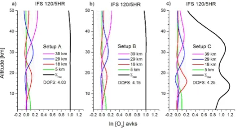
Fig. 2. Columns of the FTIR averaging kernels, avks, for retrieved ozone values using the setup A (a), setup B (b), and C (c), expressed as ln[O3], for the Iza˜na IFS 120/5HR.6row(black line) is the total

sensitivity of FTIR system and DOFS are the degrees of freedom for signal.

an ECC sonde climatology calculated from measurements between 1996 and 2006 and approximated to HALOE cli-matology above 30 km (Schneider et al., 2008b).

Setup A can be considered as the “NDACC” approach except for the logarithmic instead of the linear scale re-trieval of ozone. This strategy has already been used for the ozone trend estimations at Iza˜na and Kiruna as presented in Vigouroux et al. (2008) (updated in WMO, 2011). Setup B is further refined by an additional temperature retrieval, for which we simultaneously fit four CO2 microwindows

be-tween 962 and 970 cm−1. Schneider and Hase (2008) demon-strated that such temperature retrieval is very important when aiming for high quality ozone data. For the setups A and B the inversion problem is solved using an ad-hoc Tikhonov-Phillips slope constraint (TP1 constraint). This constrains the vertical profile slope and the absolute value for the upper-most atmospheric model altitude. The strength of the con-straint is determined by starting with a weak concon-straint and then increasing it until we observed a significant increase in the residual of the spectral fit (L-curve criterion). This is different to setup C, for which an Optimal Estimation (OE) constraint instead of the ad-hoc TP1 constraint is used. In this case, the a priori covariance matrix, Sa, is taken from

an ECC sonde climatology (Schneider et al., 2008b). In ad-dition, setup C includes an inter-species constraint between the different ozone isotopologues (666O3,686O3and668O3,

(4)

Table 1. Description of FTIR ozone retrieval setups. Note that the level of refinement increases from the setup A to the setup C.1Four temperature microwindows (MW) with isolated CO2signatures [cm−1]: 962.80–963.80, 964.25–965.25, 967.20–968.20, 968.60–969.60.

Retrieval Setup A: “NDACC” B + Temperature C + (TP→OE)

MW[cm−1] 1000–1005 1000–1005 + Temp. MW1 1000–1005 + Temp. MW1 Interfering species 666O3,686O3,668O3 666O3,686O3,668O3 666O3,686O3,668O3

H₂O, CO₂, C₂H₄ H₂O, CO₂, C₂H₄ H₂O, CO₂, C₂H₄

Logarithmic scale Yes Yes Yes

Temp. retrieval No Yes Yes

Int.-Spec. Const. No No Yes

Inversion method Tikhonov-Phillips (TP) with Tikhonov-Phillips (TP) with Optimal Estimation (OE) with slope constraint (TP1) slope constraint (TP1) Safrom Tenerife’s ECC sondes

variability, this constraint might also be advantageous for trend estimations.

For all setups H2O, CO2and C2H4are considered as main

interfering absorbers. Spectroscopic line parameters of these interfering absorbers as well as of ozone are taken from the HITRAN 2008 database (Rothman et al., 2009), except for H2O, where the parameters from the HITRAN 2009 update

are applied. The a priori mean profiles of the interfering absorbers are taken from the WACCM climatology (Whole Atmosphere Community Climate Model, http://waccm.acd. ucar.edu) provided by James W. Hanningan (National Center for Atmospheric Research).

It is important to mention that we do not vary any of the a priori trace gas profiles that depend on the season. Thereby, all variability observed in our retrieved ozone profiles comes from the measurements. As a priori for the temperature re-trievals, we use the diurnal radiosondes (Vaisala RS92) up to 30 km and extended it by the NCEP (National Centers for Environmental Prediction) 12:00 UT daily temperature pro-files. The radiosondes are launched twice per day (23:15 UT and 11:15 UT), just about 15 km southeast of the Iza˜na Ob-servatory on the coastline.

For all retrievals, we apply the ILS (Instrumental Line Shape: the interferometer’s modulation efficiency and phase error) as derived regularly from low pressure gas cell mea-surements by means of the code LINEFIT (Hase et al., 1999). 3.2 Vertical resolution of FTIR ozone profiles

The vertical structures that are detectable by a ground-based FTIR system are given by the averaging kernel matrix (avks,

ˆ

A). The columns of this matrix describe how an atmospheric perturbation is smoothed out by the remote-sensing system. As example, Fig. 2 depicts the avks columns for a typi-cal measurement of the IFS 120/5HR and for setups A, B, and C. We can observe that the maxima of these response functions generally peak at the altitude of the perturbations: the green line describes the response for an 1.0 disturbance at 5 km and it peaks close to 5 km, the red line represents the response on a disturbance at 18 km and it peaks close to 18 km, etc. The different widths of the avks and the different

Table 2. Mean (M) and standard deviation (σ) of the DOFS time series of the retrieved ozone obtained from the Iza˜na IFS 120/5HR for all setups. These values are shown for each layer (2.37–13 km, 12–23 km, 22–29 km, 28–42 km) and for the total column (2.37– 120 km).

Layer Retrieval Setup

[km] A B C

M,σ M,σ M,σ

2.37–13 1.01, 0.06 1.09, 0.05 1.31, 0.08 12–23 1.10, 0.06 1.23, 0.08 1.49, 0.11 22–29 1.01, 0.06 1.06, 0.05 1.02, 0.05 28–42 1.25, 0.06 1.28, 0.06 1.18, 0.06 2.37–120 3.84, 0.23 4.10, 0.14 4.20, 0.17

sensitivities (sum along the row of the avks,6row) are mainly

due to the differences in the applied a priori constraint. For all setups, and for altitudes below 40 km, the sensitivity is better than 80 %. Beyond 40 km the sensitivity significantly decreases for setup C, whereas for the setups A and B it re-mains very close to 1.0 (which is a typical behaviour for TP1 constraints).

(5)

Fig. 3. Time series of total DOFS of retrieved ozone values using the setup C for the whole FTIR time series between 1999 and 2010 (number of data,N, is 1887).

and B profiles. This is a consequence of the rather loose constraint applied for setup C at these altitudes (the con-straint of setup C is based on real ozone data, which show high variabilities from 15 to 25 km due to a vertically shift-ing tropopause). In addition, includshift-ing a simultaneous tem-perature fit improves the retrieval quality (i.e., reduces the residues of the fitted spectra), thus, allowing for a more de-tailed interpretation of the spectra (see also the increased DOFS when including the temperature fit).

When interpreting the FTIR ozone profile time series it is important to consider that trends in the sensitivity of the remote-sensing system (avks or DOFS) can influ-ence the ozone trend: decreasing DOFS might underestimate gradually increasing differences between the a priori ozone amounts used as constraint and the real ozone amounts, i.e., the ozone trends will be underestimated. Furthermore, there might be a bias between the climatologic ozone data (the a priori) and the FTIR ozone data due to systematic error sources like spectroscopic line parameters. In this case, the magnitude of the bias will decrease with decreasing DOFS, thereby leading to a trend even though real atmospheric ozone remains stable. The variability and the drifts in the DOFS can be observed in Fig. 3, which shows the time se-ries of the total DOFS for setup C. The apparent drift be-tween 1999 and 2004 means that trends estimated for this time period have to be treated with care. The DOFS time se-ries also shows some kind of annual cycle, which is strongly anti-correlated with the annual cycle of the ozone slant col-umn amounts (for low slant colcol-umns – less saturated ozone lines – the DOFS is higher than for high slant columns – par-tially saturated ozone lines). Likewise, in 2005 the change from the IFS 120M to the IFS 120/5HR instrument can be observed in the DOFS time series. As expected, we observe that the DOFS obtained from IFS 120M spectra are smaller than the DOFS obtained from the IFS 120/5HR spectra: the total DOFS values differ by 7 %. This difference is smaller in the troposphere (6–7 %) than in the stratosphere (up to 10 %).

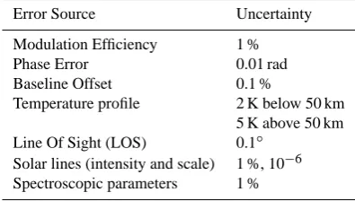
Table 3. Assumed experimental and temperature uncertainties.

Error Source Uncertainty

Modulation Efficiency 1 %

Phase Error 0.01 rad

Baseline Offset 0.1 %

Temperature profile 2 K below 50 km 5 K above 50 km Line Of Sight (LOS) 0.1◦

Solar lines (intensity and scale) 1 %, 10−6 Spectroscopic parameters 1 %

3.3 Error estimation

The theoretical error estimation is analytically performed by the retrieval code PROFFIT (Hase et al., 2004). It is based on the formalism suggested by Rodgers (2000). We consider three error types: (a) errors due to uncertainties in the input parameters (instrumental characteristics, spectroscopy data, etc.), (b) the smoothing error, and (c) errors due to measure-ment noise.

As uncertainties in the input parameters we assume the values as listed in Table 3. The uncertainties are split into sta-tistical and systematic contributions, 80 % and 20 %, respec-tively, except for spectroscopic parameters (line strength and pressure broadening coefficient), for which the entire uncer-tainty in the input parameter is systematic. The assumptions of Table 3 are reasonable for the IFS 120/5HR, but are very likely too optimistic for the IFS 120M (see, for instance, the discussion in Sect. 3.4). Hence, Table 3 only describes the errors for the IFS 120/5HR. For the IFS 120M the errors due to LOS (Line Of Sight) and ILS uncertainties are by a factor of 2–3 larger.

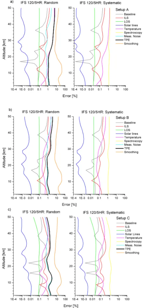
The propagation of uncertainty sources for a typical mea-surement of the IFS 120/5HR, and using the different re-trieval setups, is displayed in Fig. 4. The error profiles are shown as the root-square of the diagonal elements of the er-ror covariance matrix for the different erer-ror sources consid-ered (see Table 3). The error covariance matrices are calcu-lated following the matrix multiplication formalism as sug-gested by Rodgers (2000). The smoothing error (SE), asso-ciated with the smoothing of the real vertical distribution of ozone by the FTIR measurement process, is the leading error for all setups. It is (Aˆ−I)Sa(Aˆ −I)T, whereby I is a unity

matrix,A is the averaging kernel, and Sˆ athe assumed a

pri-ori covariance of atmospheric ozone. We use the same Sa

(6)

random errors are dominated by the measurement noise, the temperature and the ILS uncertainties. Above 20 km and for setup A the error due to temperature uncertainties notably increases, reaching about 5 % at 40 km. In contrast to the se-tups retrieving the temperature (sese-tups B and C), where the respective errors are lower than 2.5 %.

As summary, Table 4 shows the random error budget for the different partial column amounts and for the total column amount. It lists the total random errors (TRE) estimated as the root-square-sum of all parameter errors (TPE, input pa-rameters and measurement noise) and the smoothing error (SE):σTRE=

q

σ_TPE2 +σ_SE2 . The significant contributors to the TPE (ILS, temperature and measurement noise) are also shown. Note that the inclusion of a simultaneous temperature fit (setup B and C) reduces significantly the random error as-sociated with the temperature for all layers. For setup A, and especially for the higher layers (22–29 km and 28–42 km), the temperature uncertainty accounts for most of error on the ozone partial columns. This fact illustrates that a simultane-ous temperature retrieval is important when aiming on high quality middle stratospheric ozone data (Schneider and Hase, 2008). Applying the retrieval setup C, the FTIR technique provides ozone partial columns with an overall precision of better than 3 % for the tropopause and middle/upper strato-sphere and of better than 6 % for the tropostrato-sphere.

Regarding setup B and C, the spectroscopic parameters are responsible for most of the systematic errors, whereas for setup A the temperature uncertainty becomes an important systematic error source, especially above the troposphere.

High quality measurements are very important for trend studies, since they minimise possible artificial trends caused by drifts in the error sources. For example, a simultaneous temperature fit minimises the artificial trend that might be caused by a drift in the temperature uncertainty (e.g., it might be−1◦C in 2000 and gradually improve to∼0◦C in 2010). Another example is the ILS uncertainty (see Fig. 4). If a possible drift in the ILS is not adequately considered in the retrieval an artificial trend will be the consequence (in the following subsection, we demonstrate that it is very impor-tant to regularly monitor the ILS by laboratory cell measure-ments). Furthermore, a realistic constraint assures a correct interpretation of the variability as seen in the measured spec-tra, thereby leading to ozone data of a best possible quality (compare error budgets of setup B and C).

3.4 Long-term consistency of the ILS

Figure 4 shows that the ILS uncertainties are an important error source (in particular, middle and upper stratosphere). When aiming on a consistent long-term quality of ozone pro-files, a continuous and precise documentation of the ILS is mandatory. Therefore, at Iza˜na we make regular low pres-sure N2O cell measurements. These measurements allow for

retrieving the actual ILS by means of the LINEFIT code

(7)

Table 4. Estimated random errors relative to actual ozone partial columns and total column [%] for the Iza˜na IFS 120/5HR for all setups and for the different layers.

[km] A B C

TPE (ILS, Temp, Noi), SE, TRE TPE (ILS, Temp, Noi), SE, TRE TPE (ILS, Temp, Noi), SE, TRE

2.37–13 1.0 (0.4, 0.6, 0.8), 7.1, 7.2 0.9 (0.4, 0.5, 0.6), 6.8, 6.9 1.0 (0.3, 0.5, 0.8), 5.5, 5.6 12–23 1.4 (0.4, 1.3, 0.5), 2.4, 2.8 0.7 (0.5, 0.3, 0.4), 2.3, 2.4 0.7 (0.5, 0.3, 0.4), 1.8, 1.9 22–29 2.7 (<0.1, 2.7, 0.4), 3.2, 4.2 0.9 (0.6, 0.3, 0.5), 3.2, 3.3 0.9 (0.5, 0.3, 0.5), 2.8, 2.9 28–42 4.3 (0.7, 4.2, 0.5), 3.4, 5.5 2.0 (1.6, 0.7, 0.7), 2.9, 3.5 1.6 (1.3, 0.6, 0.6), 2.4, 2.9 2.37–120 2.3 (0.1, 2.3, 0.1), 0.2, 2.3 0.7 (0.4, 0.4, 0.2), 0.1, 0.7 0.6 (0.4, 0.3, 0.2), 0.2, 0.6

TPE [%]: Total Parameter Error due to input parameters and measurement noise; ILS [%]: Error due to instrumental line shape; Temp [%]: Error due to temperature; Noi [%]: Error due to measurement noise; SE [%]: Smoothing Error; TRE [%, in bold]: Total Random Error.

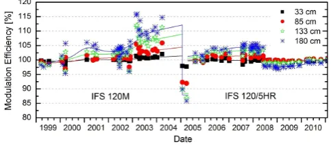
Fig. 5. Times series of the modulation efficiency [%] at different op-tical path differences (OPD) for the Iza˜na spectrometers. Individual data points indicate individual cell measurements. The lines are the smoothed efficiency curves used during the FTIR retrievals. Black at 38 cm, red at 85 cm, green at 133 cm and blue at 180 cm.

(Hase et al., 1999). LINEFIT estimates the ILS at 20 equidis-tant optical path intercepts. At Iza˜na we have performed such cell measurements about every two months. Figure 5 shows the 1999–2010 time series of the modulation efficiency ob-tained for the two spectrometers. The jumps in the time se-ries (beginning of 2005 for IFS 120M and June 2008 for the IFS 120/5HR) are due to realignments of the instruments.

As expected, we observe that the ILS of IFS 120M is sig-nificantly less stable than the ILS of IFS 120/5HR. While for the IFS 120/5HR the modulation efficiency can be de-termined with a precision of about 1 %, for the IFS 120M we only achieve a precision of 3 %. Concerning the phase error, we make a similar observation: with our regular cell measurements we can achieve a precision of 0.005 rad for the IFS 120/5HR, but only of 0.025 rad for the IFS 120M. It is important to note we apply the ILS as obtained from the cell measurement for our ozone retrieval. Otherwise, the re-sulting error in the ozone profiles would be much larger than estimated in Fig. 4 and Table 4.

3.5 Comparison between IFS 120M and IFS 120/5HR

During March and April 2005 both instruments (IFS 120M and IFS 120/5HR) measured side-by-side. The comparison between these coincidental measurements is displayed in Fig. 6, where the ozone partial columns as obtained from re-trieval setup C are shown.

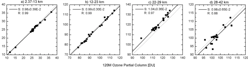
The agreement is excellent, except for the highest layers, where the FTIR data are more sensitive to instrumental un-certainties (ILS and measurement noise, see Fig. 4). For ex-ample, we observe a mean ratio between the IFS 120/5HR and 120M data of 0.98±0.39×10−2(±1 standard error of the mean value) with a correlation of 99 % in 2.37–13 km layer and 0.98±0.65×10−2 with a correlation of 88 % in 28–42 km layer. These values are for setup C results. When comparing the IFS 120M and IFS 120/5HR results obtained by retrieval setups A and B, we find more scatter and lower correlation coefficients at the highest altitudes. This is ex-pected from the error estimation (more uncertainty in setup A and B than in setup C retrieval data, see Table 4). Note also that higher errors are expected for the IFS 120M ozone re-trievals due to its higher ILS uncertainties (see Fig. 5) and its higher measurement noise and, consequently, lower sensitiv-ity. The lower sensitivity is clearly observed by comparing the DOFS time series of retrieved ozone from the two spec-trometers (see Fig. 3).

(8)

Table 5. Statistics of coincident measurements from the IFS 120/5HR and IFS 120M ozone partial columns for each setup and layer (N=19).

[km] A B C

M±SEM,σ,S,R M±SEM,σ,S,R M±SEM,σ,S,R

2.37–13 −0.3±0.4, 1.8, 1.00±0.42×10−2, 0.99 +2.8±0.4, 2.0, 0.97±0.41×10−2, 0.99 −2.6±0.4, 1.9, 0.98±0.39×10−2, 0.99 12–23 +1.0±0.4, 1.6, 0.99±0.36×10−2, 0.99 +1.4±0.3, 1.4, 0.99±0.32×10−2, 0.99 +1.1±0.3, 1.3, 0.99±0.30×10−2, 0.99 22–29 −6.2±0.4, 1.9, 1.07±0.48×10−2, 0.96 −4.0±0.4, 1.7, 1.04±0.41×10−2, 0.97 −3.7±0.3, 1.5, 1.04±0.36×10−2, 0.97 28–42 −3.5±0.8, 3.4, 1.04±0.83×10−2, 0.78 +0.4±0.7, 2.9, 1.00±0.63R−2, 0.84 +1.7±0.6, 2.4, 0.98±0.65×10−2, 0.88 M±SEM [%]: mean and standard error of the mean of relative differences (120M-120/5HR)/120/5HR;σ[%]: standard deviation of relative differences;S: slope of the linear regression trough origin;R: correlation coefficient of the linear fit.

Fig. 6. Comparison between the IFS 120/5HR and IFS 120M ozone partial columns [DU] for the 120M-120/5HR coincidences during March and April 2005 (N=19) and for setup C: (a) 2.37–13 km, (b) 12–23 km and (c) 22–29 km and (d) 28–42 km. The black solid lines are the linear regression lines through origin, whose parameters are shown in the legend (S is the slope of regression fit and R the correlation coefficient). The dotted lines are the diagonals.

4 Consistency of ECC sonde time series

Before using the ECC data as reference for empirically as-sessing the quality of the FTIR ozone data and their represen-tativeness for annual cycles and trends, it is very important to check the consistency of the ECC ozone time series. In this section, we use the coincident measurements of ozone to-tal column from Brewer spectrometers and of surface ozone from in situ analysers for empirically documenting the qual-ity and the long-term stabilqual-ity of the ECC sonde dataset. 4.1 ECC sonde vs. Brewer

The consistency and quality of the ECC sonde ozone pro-file (xECC org) time series can be estimated by comparing

it to independent and coincident very high quality mea-surements of ozone total amounts. At the Iza˜na Observa-tory such high quality measurements are performed by the FTIR system and by Brewer spectrometers. The Brewers have been operative since May 1991, and like the ECC sonde and FTIR Programs, they have been part of NDACC since March 2001. Furthermore, since November 2003 they rep-resent the Regional Brewer Calibration Center for Europe (http://www.rbcc-e.org/) of WMO/GAW, which guarantees the high quality of their ozone total column measurements (better than 1 %, Redondas and Cede, 2006).

The ECC sondes normally burst between 30 and 34 km. In order to homogenise the study, we only consider the ECC data measured up to 29 km. Thus, the ozone total columns from the ECC sondes (TCECC org) have been calculated by

integrating the ozone profiles up to 29 km and adding a typ-ical residual ozone column up to the top of atmosphere. This residual has been estimated from the mean difference between the daily Brewer total ozone columns (TCBrewer)

and ECC ozone partial amounts up to 29 km (PCECC org)

for all 515 Brewer/ECC coincidences from 1999 to 2010 (for more details see Schneider et al., 2008b). We found a mean and a standard deviation (1σ) for the ozone residual of 81.5 and 10.6 DU, respectively. Note that in our study, we apply Brewer measurements in order to remain independent from the FTIR data.

The Brewer total ozone columns can be used to correct the ECC sonde profiles (xECC) by:

xECC=_PCTCBrewer

ECC org+81.5 ·xECC org= CF·xECC org (1)

whereby CF (CF= TCBrewer

PCECC org+81.5) is the daily correction

fac-tor. Schneider et al. (2008b) illustrated that by this correction the quality of the ECC data can be significantly improved.

(9)

Fig. 7. Time series of correction factor (CF, according to Eq. 1) at the Iza˜na Observatory (a) and of ozone total col-umn amounts from ECC sondes without and with correction (TCECC=CF·TCECC org) (b). The mean correction factors for the

periods 1999–2004 and 2005–2010 are also shown. The black ar-rows indicate the change-point date.

2005–2010, respectively. Such systematic change of about

−4 % between the ECC records can be expected by chang-ing the senschang-ing solution type or ECC sonde type (Smit et al., 2007, and references therein). During 2005 the sensing solu-tions in the ECC sondes were substituted by a new batch, but the same manufacturer’s operating procedures, and ratio of cathode sensing solutions, have been kept during whole pe-riod (1999–2010). Nonetheless, in the light of above results, we might assume that some change in the sensing solutions was introduced by using the new batch. The discontinuities in the CF time series is also identified by a rank order change point test (Lanzante, 1996; Romero et al., 2011). This non-parametric method, based on the ranks of the monthly values from a time series, is not particularly affected by gaps and outliers in the time series.

The time series of ECC ozone total columns, without and with correction (TCECC organd TCECC, respectively), is

dis-played in Fig. 7b. The corrected ECC records benefit from the synergies of the two techniques: the high vertical resolu-tion of the ECC sondes and the high precision of the Brewer measurements.

4.2 ECC sonde vs. surface

At the Iza˜na Observatory the tropospheric surface ozone is also monitored by photometric in situ analysers. This surface dataset can also be used for documenting the long-term con-sistency of the ECC sonde profiles at Iza˜na’s altitude.

In order to evaluate possible drifts in the ECC sonde dataset, we examine the time series of the differences in the monthly means between the ECC and the photometric

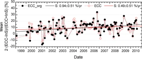
Fig. 8. Monthly mean time series of the relative differences [%] be-tween the ozone VMR from the ECC sonde data (corrected, ECC, and not corrected by the daily CF, ECC org,) at Iza˜na’s altitude and surface data (N=112). The solid lines are the linear regression lines of the least square fits. The slopes and the 95 % confidence ranges (±2σ) are shown in the legend (S).

surface data (Fig. 8). To do so the photometric surface data were averaged 30 min around the ECC measurements. For the ECC data corrected according to Eq. (1), the drift, i.e., the trend in the differences is not significant (0.49±0.51 % yr−1). On average, we find a mean bias and a scatter (1σ) of 10 % and 15 %, respectively, between the two techniques. Note that, if the ECC profiles are not corrected, we observed a significant drift in the difference between the ECC and the photometric surface data (0.94±0.51 % yr−1_),

confirming the importance of correcting the ECC time series before using it for long-term studies.

Both the Brewer and the photometric surface measure-ments identify a jump in the ECC time series. This jump would significantly affect the estimated ozone trends as well as the inter-comparison with another technique. Therefore, in the subsequent analysis we will exclusively apply the cor-rected ECC sonde time series (corcor-rected according to Eq. 1).

5 Validation of FTIR ozone profiles

(10)

Fig. 9. Relative differences [%] between the ozone partial columns (2.37–13 km, 12–23 km and 22–29 km) calculated from the ECC sonde and from the different FTIR setups: (a) mean values (error bars indicate the standard error of the mean) and (b) scatter or stan-dard deviation (1σ). It is also shown the differences between the FTIR and Brewer ozone columns.Xmeans the ECC or Brewer data.

two completely independent datasets, which would not be the case if we smooth the ECC data by the FTIR’s avks.

The straightforward comparison of ozone partial columns from FTIR and corrected ECC sondes is rather satisfac-tory, as shown in Fig. 9. We find a mean bias between

−8 % and−4 % in troposphere (2.37–13 km), about 1 % in the tropopause region (12–23 km) and about 7 % in mid-dle stratosphere (22–29 km) for all retrieval setups, while the scatter is between 6 % and 9 % for the two first layers and only of 3 % in middle stratosphere (see Fig. 9a and b). These results rather agree with the expected uncertainty for the ECC sondes given by Smit et al. (2007) (±5–10 %) and with our FTIR theoretical error estimation (Sect. 3.3). Furthermore, they are in good agreement with other inter-comparison studies using ECC sonde data (Calisesi et al., 2005; Nair et al., 2011 and references therein). It illustrates the good agreement between the ECC sonde and FTIR tech-niques. As example, Fig. 10 shows the direct comparison be-tween the coincident FTIR (setup C) and ECC sonde partial columns from 1999 to 2010 (N=262).

Part of the discrepancy observed between FTIR and ECC sonde measurements is due to the smoothing error (recall Ta-ble 4). Smoothing the ECC sonde profiles with the FTIR avks improves the agreement for all setups by reducing the scat-ter, on average, to 7 %, 5 % and 2 % for the 2.37–13 km, 12– 23 km and 22–29 km layers, respectively. Other sources of discrepancy might be errors in the FTIR and/or ECC data and the observation of different air masses by the FTIR ex-periment, on the one hand, and ECC exex-periment, on the other (Schneider et al., 2008b). The systematic discrepancies might be attributable to systematic ECC and FTIR errors

caused, for instance, by uncertainties in the spectroscopic line parameters.

It is important to note that the scatter between FTIR and ECC concentrations decreases as the level of refinement of setups increases, especially in the troposphere and the tropopause region. Due to the reduction of the temperature error and the use of a realistic constraint, setup C provides the FTIR profiles that best agree with the ECC sonde profiles. This is in good agreement to our theoretical estimation as presented in Table 4 and Fig. 4. As addendum to the com-parison to the ECC data, Fig. 9 shows the comcom-parison to the Brewer data that have been used in the Schneider et al. (2008a) paper. We observe that the scatter between the FTIR and Brewer ozone total column amounts is significantly re-duced (from 1.06 % to 0.71 %) as the FTIR setups become more refined, confirming the results of the FTIR-ECC com-parison. Similar results were found for the comparison be-tween FTIR and Iza˜na’s surface data, i.e., the best agreement is obtained for the retrieval setup C. We find a scatter (1σ) of 20 % for the setup C and of 23 % for setup A. The scatter between the ECC sonde and Iza˜na’s surface data is smaller (15 %, recall Sect. 4.2). The slightly increased scatter when comparing with the FTIR is due to the FTIR’s smoothing er-ror.

In order to evaluate possible artificial trend in the FTIR’s DOFS time series, we analyse the time series of the differ-ences between smoothed and unsmoothed ECC sonde data. This can be done for the 262 occasions during the 1999–2010 time period where FTIR and ECC measurements are per-formed in coincidence. For all setups, we observe that there are no significant trends in the 2.37–13 km and 12–23 km lay-ers, but that there is a significant trend (at 95% of confidence) for the 22–29 km layer. For example, for setup C, the trend is of 0.12±0.10 DU yr−1 (i.e., 0.11±0.09 % yr−1), which might indicate that drifts in the avks affect the Iza˜na 1999– 2010 middle/upper stratospheric FTIR ozone trend. These facts consolidate our applied strategy not to smooth the ECC sondes for trend comparisons. Otherwise, both instruments might show similar trends, due to the fact that there is a trend in the avks. However, we also have to consider that the data subset of ECC/FTIR coincidences is not well representative for the whole FTIR time series (the number of coincidences is rather small and most of them occur from April to Octo-ber).

6 Trends and seasonality

6.1 Ozone trends

(11)

Fig. 10. Comparison between the ozone partial columns from FTIR (setup C) and ECC sonde data (N=262): (a) 2.37–13 km, (b) 12–23 km and (c) 22–29 km. The black solid lines are the linear regression line of the least square fits, whose parameters are shown in the legend (S andBare the slope and the bias of the regression fit, respectively, andRthe correlation coefficient). The dotted lines are the diagonals.

Fig. 11. Time series of FTIR ozone partial columns [DU] (setup C) for the different layers. Black dots: individual measurements (N=1887); Red lines: annual cycle according to Eq. (2).

ground-based FTIR ozone trends and examines its consis-tency to trends obtained from ECC sonde and surface in situ analyser datasets.

The ozone trends are estimated by using a bootstrap re-sampling method (Gardiner et al., 2008), which models the total variation in ozone by a functionF (t ) and allows for separating the annual cycles from possible long-term trends:

F (t )=fo+ftrendt + p P

i=1

[aicos(ωit )+bisin(ωit )] (2)

wheret is measured in years,fo is a baseline constant and

ftrend the linear trend in change per year. The annual

cy-cle is modelled in terms of a Fourier series where ai and

bi are the parameters of the Fourier series to be determined

andωi=2π i/T with T=365.25 days. We consider

fre-quencies up to 3 yr−1(p=3), since the third order Fourier series provided the best overall results (Gardiner et al., 2008;

Fig. 12. Linear trends (% yr−1) between 1999 and 2010 for the FTIR (N=1887), the corrected ECC sonde (N=515) and surface in situ (N=42415) datasets. The error bars indicate the 95 % con-fidence ranges (±2σ).

Vigouroux et al., 2008). Figure 11 shows the FTIR ozone time series (setup C) and the fitted functionF (t )for the dif-ferent layers.

Although our bootstrap model does not capture atmo-spheric processes such as quasi-biennial oscillations (QBO) or solar cycle variations (e.g., Reinsel et al., 2002), they be-come a noise source in the linear trend determination and, thus, feed into the uncertainties in the determined trends (Vigouroux et al., 2008). The significance of linear trends is estimated by assuming that the residuals are Gaussian and uniform over the whole analysed time period (Gardiner et al., 2008).

(12)

Fig. 13. Annual cycle of the ozone partial columns [DU] obtained from the FTIR (setup A and C), the corrected ECC sonde data (not smoothed and smoothed by avks from the FTIR setup A and C): (a) 2.37–13 km, (b) 12–23 km, (c) 22–29 km and (d) 28–42 km. The error bars indicate the standard error of the mean value.

retrieval (setup B and C), whereas the setup A dataset indi-cates a positive trend. In order to get more insight into the long-term evolution of this tropospheric layer, we have also estimated the ozone trends from the night-time surface in situ data, whose for Iza˜na are well representative of the free tro-posphere conditions. Thus, the airmass detected by the in situ technique can be compared to the tropospheric airmass re-motely sensed by the FTIR system (Sep´ulveda et al., 2012). We observe a significant small negative trend (see Fig. 12), which better agrees with the setups that simultaneous fit the temperature profile. In summary, the trends obtained from the setup C datasets tend to be in better agreement with the trends obtained from the ECC sonde and surface in situ datasets, al-though the differences to the trends estimated from setup A and B datasets are rather small.

It is interesting to mention that the significant ozone trends observed by the FTIR system in the upper troposphere/lower stratosphere (negative trend) and in the middle/upper strato-sphere (positive trend) are also predicted by current climate models at the northern subtropical latitudes (Hegglin and Shepherd, 2009; Li et al., 2009). For example, Li et al. (2009) estimate that a decrease of ozone is to be expected in the lower stratosphere in the northern subtropical latitudes associated with the predicted increase in the stratospheric Brewer-Dobson circulation. An accelerated Brewer-Dobson circulation transports more ozone from tropics to the mid-high latitudes and could delay ozone recovery in the trop-ics and advanced ozone recovery in the extra-troptrop-ics. How-ever, we have to be aware that a 12-yr time series might be too short for validating the models due to the large year-to-year variability of this stratospheric circulation (Weber et al., 2011). Likewise, Li et al. (2009) show that the photochemical response to strong cooling induced by increasing greenhouse gases concentrations would lead to an upper stratospheric ozone increase. In addition, the leveling off of anthropogenic halogen components in the upper stratosphere since the mid-1990s has to be considered (WMO, 2007). Similar results were reported by WMO (2011).

For the upper stratosphere the quality of the FTIR ozone time series has not been empirically validated in this work

by day-to-day intercomparisons due to the lack of respective ECC data. Previous campaign studies show good agreement between the ozone measurements obtained from FTIR and other measurement techniques in this layer, such as ground-based LIDAR and millimeter-wave radiometer (Kopp et al., 2002; Vigouroux et al., 2008). However, at these altitudes the FTIR ozone data are very sensitive to ILS uncertainties and to measurement noise. Consequently, our upper stratospheric trend estimations should be treated with care, although they are consistent for all setups and are supported by other experimental studies. For example, Steinbrecht et al. (2009) found that the upper stratospheric ozone (35–45 km) has been slightly increasing since the late 1990s at other NDACC sites at similar latitudes (Mauna Loa, 19.5◦N 155.6◦E, and Ta-ble Mountain, 34.5◦_{N 117.7}◦_{E), using satellite- and}

ground-based LIDAR measurements. This stratospheric ozone re-covery has also been documented experimentally by FTIR records in northern subtropical, middle and polar latitudes (updated from Vigouroux et al., 2008 in WMO, 2011). 6.2 Ozone annual cycle

The annual ozone cycles have been calculated by produc-ing monthly averages considerproduc-ing the whole time series. Fig-ure 13 shows the annual cycles for the FTIR data (setup A and C) and the corrected ECC sonde data (not smoothed and smoothed by avks from the FTIR setup A and C). We observe that the agreement between the two techniques is rather sat-isfactory.

(13)

observed in the middle/upper stratosphere (22–29 km and 28–42 km). There we observe maximum ozone concentra-tions in summer-autumn when the tropical condiconcentra-tions prevail. In the middle stratosphere the FTIR system detects a maxi-mum in spring that is not found in the ECC sonde annual cycle. This is due to the smoothing error: the FTIR ozone partial column in this layer contains information from the lower layers (12–23 km), where the spring maximum is due to the annual cycle in the tropopause altitude.

Note that applying different constraints and temperature retrievals do not significantly affect the ozone seasonality.

7 Conclusions

In this paper, we document the quality of the ozone profiles obtained from ground-based FTIR systems and discuss its application for long-term studies. We investigate three dif-ferent retrieval setups: (A) an ad-hoc constraint for ozone and no temperature profile retrieval, (B) an ad-hoc constraint for ozone and a simultaneous temperature profile retrieval, and (C) an ozone constraint based on an ozone climatology (optimal estimation retrieval) and a simultaneous tempera-ture profile retrieval.

Our theoretical error assessment reveals that the measure-ment noise and the uncertainties in the ILS and the ap-plied temperature profile (for setup A) are the leading er-ror sources. In particular, the retrieved middle/upper strato-spheric ozone amounts are strongly affected by ILS and tem-perature uncertainties. We show that the temtem-perature error can be significantly reduced by performing a simultaneous temperature profile retrieval. Moreover, the ad-hoc constraint retrievals offer more DOFS in the middle/upper stratosphere than the optimal estimation retrieval. At lower altitudes it is vice versa. An optimal estimation retrieval is supposed to interpret the measured spectra in a best possible manner. Consequently, the ad-hoc constraint retrievals might misin-terpret ozone variability (over-/under-estimate variability at higher/lower altitudes).

For an empirical quality assessment, we use a coincident ECC sonde ozone profile dataset as reference, whose qual-ity, in turn, has been checked, independently from the FTIR data, by a comparison to Brewer total column and surface in situ measurements. During the 12-yr period of 1999–2010, the agreement between the vertical ozone distribution ob-tained by the FTIR and the ECC sondes is very satisfac-tory. We show empirically that the FTIR system is well able to capture the day-to-day ozone variability in the tro-posphere, tropopause region and middle stratosphere. Fur-thermore, both techniques reveal very similar annual season-ality. For the ozone retrieval setup that applies a constraint based on an ozone climatology and includes a simultane-ous temperature profile retrieval we observe a slightly better agreement than for the other setups. These observations con-firm our theoretical quality assessment.

Regarding ozone trends, we estimate the trends for the 1999–2010 time period for the ECC, surface in situ analy-sers, and FTIR datasets. In the middle stratosphere we ob-serve a significant positive trend (95 % confidence interval) for the ECC and for all three FTIR datasets (the FTIR also reveals a significant positive trend above 30 km, where there are no ECC data available). In the upper troposphere/lower stratosphere region the FTIR observes a significant negative trend (95 % confidence interval), which cannot be confirmed by the ECC dataset. At these altitudes ozone amounts are very variable and the trend estimates are rather uncertain. This is especially true for the ECC trend estimates, since there is only one ECC observation per week. FTIR obser-vations are made more frequently (several times per week), leading to smaller uncertainties in the trend estimates. In the troposphere we observe no significant trend neither in the ECC nor in the FTIR datasets. The surface in situ data re-veal a significant negative trend, which is interestingly also indicated by the two FTIR retrieval setups that apply a simul-taneous temperature retrieval.

A main reason for this satisfactory agreement is the fact that we take a lot of care in documenting the ILS (see Fig. 5), thereby avoiding artificial trends due to drifts in the ILS. A regular ILS monitoring, applying low pressure gas cell mea-surements, is very important for FTIR trend studies of strato-spheric absorbers. Furthermore, we think that a simultaneous temperature retrieval is important, since it can significantly reduce the risk of artificial trends caused by possible drifts in the temperature uncertainty, thereby theoretically increasing the reliability of the FTIR trends. In our study, we observe that the temperature retrieval modifies the estimated trends. Using a realistic constraint instead of an ad-hoc constraint is important for reproducing the large day-to-day variability (see comparisons in Sect. 5), and it also slightly affects the estimated trends. Finally, one should consider the temporal evolution of the DOFS when using remote-sensing data for trend studies. For example, if there is a bias in the remote-sensing data, this bias will very likely decrease with decreas-ing DOFS, thereby givdecreas-ing rise of an artificial trend.

(14)

Acknowledgements. Since 1999 the Izaña FTIR activities have been supported by different funding agencies: European Commis-sion, European Space Agency, Deutsche Forschungsgemeinschaft, Deutsches Zentrum für Luft- und Raumfahrt, and the Ministerios de Ciencia e Innovación and Educación from Spain. Furthermore, the research leading to these results has received funding from the European Community’s Seventh Framework Program ([FP7/2007-2013]) under grant agreement no. 284421 (see Article II. 30. of the Grant Agreement). We are grateful to the Goddard Space Flight Center for providing the temperature and pressure profiles of the National Centers for Environmental Prediction. M. Schneider is supported by the European Research Council under the European Community’s Seventh Framework Program (FP7/2007-2013)/ERC Grant agreement no. 256961 and E. Sepúlveda enjoys a pre-doctoral fellowship from the Spanish Ministry of Education. Finally, the authors would like thank Carlos Marrero and Pedro M. Romero for their useful comments.

Edited by: M. Weber

References

Anderson, J. G., Wilmouth, D. M., Smith, J. B., and Sayres, D. S.: UV Dosage Levels in Summer: Increased Risk of Ozone Loss from Convectively Injected Water Vapor, Science, 835–839, 2012.

Barret, B., De Mazi`ere, M., and Demoulin, P.: Retrieval and char-acterization of ozone profiles from solar infrared spectra at the Jungfraujoch, J. Geophys. Res., 107, 4788–4803, 2002. Calisesi, Y., Soebijanta, V., and van Oss, R.: Regridding

of remote soundings: Formulation and application to ozone profile comparison, J. Geophys. Res., 110, D23306, doi:10.1029/2005JD006122, 2005.

Gardiner, T., Forbes, A., de Mazi`ere, M., Vigouroux, C., Mahieu, E., Demoulin, P., Velazco, V., Notholt, J., Blumenstock, T., Hase, F., Kramer, I., Sussmann, R., Stremme, W., Mellqvist, J., Strand-berg, A., Ellingsen, K., and Gauss, M.: Trend analysis of green-house gases over Europe measured by a network of ground-based remote FTIR instruments, Atmos. Chem. Phys., 8, 6719–6727, doi:10.5194/acp-8-6719-2008, 2008.

Hase, F., Blumenstock, T., and Paton-Walsh, C.: Analysis of the instrumental line shape of high-resolution Fourier transform IR spectrometers with gas cell measurements and new retrieval soft-ware, Appl. Optics, 38, 3417–3422, 1999.

Hase, F., Hanningan, J. W., Coffey, M. T., Goldman, A., H¨ofner, M., Jones, N. B., Rinsland, C. P., and Wood, S. W.: Intercomparison of retrieval codes used for the analysis of high-resolution ground-based FTIR measurements, J. Quant. Spectrosc. Ra., 87, 25–52, 2004.

Hegglin, M. I. and Shepherd, T. G.: Large climate-induced changes in ultraviolet index and stratosphere-to troposphere ozone flux, Nat. Geosci., 2, 687–691, doi:10.1038/NGEO604, 2009. Johnson, D., Jucks, K., Traub, W., and Chance, K.: Isotopic

compo-sition of stratospheric ozone, J. Geophys. Res., 105, 9025–9031, 2000.

Kopp, G., Berg, H., Blumenstock, T., Fischer, H., Hase, F., Hochschild, G., H¨opfner, M., Kouker, W., Reedmann, T., Ruhnke, R., Raffalsky, U., and Kondo, Y.: Evolution of ozone and ozone-related species over Kiruna during the SOLVE/THESEO

2000 campaign retreived from ground-based milimeter-wave and infrared observations, J. Geophys. Res., 107, 8308, doi:10.1029/2001JD001064, 2002.

Kurylo, M. J. and Zander, R.: The NDSC-Its status after 10 years of operation, in: Proceedings of XIX Quadrennian Ozone Sympo-sium, Hokkaaido University, Sapporo, Japan, 167–168, 2000. Lanzante, J. R.: Resistant, robust and non-parametric techniques or

the analysis of climate data: theory and examples, including ap-plications to historical radiosonde station data, Int. J. Climatol., 16, 1197–1226, 1996.

Li, F., Stolarski, R. S., and Newman, P. A.: Stratospheric ozone in the post-CFC era, Atmos. Chem. Phys., 9, 2207–2213, doi:10.5194/acp-9-2207-2009, 2009.

Mauersberger, K., L¨ammerzahl, P., and Krankowsky, D.: Strato-spheric ozone isotope enrichments-revisited, Geophys. Res. Lett., 28, 3155–3158, 2001.

Nair, P. J., Godin-Beekmann, S., Pazmi˜no, A., Hauchecorne, A., Ancellet, G., Petropavlovskikh, I., Flynn, L. E., and Froidevaux, L.: Coherence of long-term stratospheric ozone vertical distribu-tion time series used for the study of ozone recovery at a north-ern mid-latitude station, Atmos. Chem. Phys., 11, 4957–4975, doi:10.5194/acp-11-4957-2011, 2011.

Redondas, A. and Cede, A.: Brewer algorithm sensitivity analysis, in: Sauna Workshop, Puerto de la Cruz, Tenerife, 2006. Reinsel, G. C., Weatherhead, E. C., Tiao, G. C., Miller, A. J.,

Na-gatani, R. M., Wuebbles, D. J., and Flynn, L. E.: On detection of turnaround and recovery in trend for ozone, J. Geophys. Res., 107, 4078–4090, 2002.

Rodgers, C.: Inverse Methods for Atmospheric Sounding: Theory and Praxis, World Scientific Publishing Co., Singapore, 2000. Romero, P. M., Marrero, C. L., Alonso-P´eerez, S., Cuevas, E., and

Afonso, S.: Una climatolog´ıa del agua precipitable en la regi´on subtropical sobre la Isla de Tenerife, vol. NTD CIAI-6, NIPO: 281-12-007-5, Servicio de Publicaciones de la AEMET, Madrid, Spain, 2011.

Rothman, L. S., Gordon, I. E., Barbe, A., Benner, D. C., Bernath, P. F., Birk, M., Boudon, V., Brown, L. R., Campargue, A., Cham-pion, J.-P., Chance, K., Coudert, L. H., Dana, V., Devi, V. M., Fally, S., Flaud, J.-M., Gamache, R. R., Goldmanm, A., Jacque-mart, D., Kleiner, I., Lacome, N., Lafferty, W., Mandin, J.-Y., Massie, S. T., Mikhailenko, S. N., Miller, C. E., Moazzen-Ahmadi, N., Naumenko, O. V., Nikitin, A. V., Orphal, J., Perevalov, V. I., A. Perrini, A. P.-C., Rinsland, C. P., Rotger, M., ˇSimeˇckov´a, M., Smith, M. A. H., Sung, K., Tashkun, S. A., Ten-nyson, J., Toth, R. A., Vandaele, A. C., and VanderAuwera, J.: The HITRAN 2008 Molecular Spectroscopic Database, J. Quant. Spectrosc. Ra., 110, 533–572, 2009.

Schneider, M. and Hase, F.: Technical Note: Recipe for monitoring of total ozone with a precision of around 1 DU applying mid-infrared solar absorption spectra, Atmos. Chem. Phys., 8, 63–71, doi:10.5194/acp-8-63-2008, 2008.

Schneider, M., Hase, F., and Blumenstock, T.: Ground-based re-mote sensing of HDO/H₂O ratio profiles: introduction and vali-dation of an innovative retrieval approach, Atmos. Chem. Phys., 6, 4705–4722, doi:10.5194/acp-6-4705-2006, 2006.

(15)

Schneider, M., Hase, F., Blumenstock, T., Redondas, A., and Cuevas, E.: Quality assessment of O3 profiles measured by

a state-of-the-art ground-based FTIR observing system, At-mos. Chem. Phys., 8, 5579–5588, doi:10.5194/acp-8-5579-2008, 2008b.

Sep´ulveda, E., Schneider, M., Hase, F., Garc´ıa, O. E., Gomez-Pelaez, A., Dohe, S., Blumenstock, T., and Guerra, J. C.: Long-term validation of tropospheric column-averaged CH4 mole frac-tions obtained by mid-infrared ground-based FTIR spectrometry, Atmos. Meas. Tech., 5, 1425–1441, doi:10.5194/amt-5-1425-2012, 2012.

Smit, H. G. J., Straeter, W., Johnson, B. J., Oltmans, S. J., Davies, J., Tarasick, D. W., Hoegger, B., Stubi, R., Schmidlin, F. J., Northam, T., amd J. C. Witte, A. M. T., Boyd, I., and Posny, F.: Assessment of the performance of ECC-ozonesondes under quasi-flight conditions in the environmental simulation chamber: Insights from the Juelich Ozone Sonde Intercom-parison Experiment (JOSIE), J. Geophys. Res., 112, D19306, doi:10.1029/2006JD007308, 2007.

Steinbrecht, W., Claude, H., Sch¨onenborn, F., McDermid, I. S., Leblanc, T., Godin-Beekmann, S., Keckhut, P., Hauchecorne, J. A. E. V. G., Swart, D. P. J., Bodeker, G. E., Parrish, A., Boyd, I. S., K¨ampfer, N., Hocke, K., Stolarski, R. S., Frith, S. M., Thomason, L. W., Remsberg, E. E., Savigny, C. V., Rozanov, A., and Burrows, J. P.: Ozone and temperature trends in the up-per stratosphere at five stations of the Network for the Detection of Atmospheric Composition Change, Int. J. Remote Sens., 30, 3875–3886, 2009.

Viatte, C., Schneider, M., Redondas, A., Hase, F., Eremenko, M., Chelin, P., Flaud, J.-M., Blumenstock, T., and Orphal, J.: Com-parison of ground-based FTIR and Brewer O3total column with

data from two different IASI algorithms and from OMI and GOME-2 satellite instruments, Atmos. Meas. Tech., 4, 535–546, doi:10.5194/amt-4-535-2011, 2011.

Vigouroux, C., De Mazi`ere, M., Demoulin, P., Servais, C., Hase, F., Blumenstock, T., Kramer, I., Schneider, M., Mellqvist, J., Strand-berg, A., Velazco, V., Notholt, J., Sussmann, R., Stremme, W., Rockmann, A., Gardiner, T., Coleman, M., and Woods, P.: Eval-uation of tropospheric and stratospheric ozone trends over West-ern Europe from ground-based FTIR network observations, At-mos. Chem. Phys., 8, 6865–6886, doi:10.5194/acp-8-6865-2008, 2008.

Weatherhead, E. and Andersen, S.: The search for signs of recovery of the ozone layer, Nature, 441, 39–45, 2006.

Weber, M., Dikty, S., Burrows, J. P., Garny, H., Dameris, M., Ku-bin, A., Abalichin, J., and Langematz, U.: The Brewer-Dobson circulation and total ozone from seasonal to decadal time scales, Atmos. Chem. Phys., 11, 11221–11235, doi:10.5194/acp-11-11221-2011, 2011.

WMO: Scientific Assessment of Ozone Depletion: 2006, Global Ozone Research and Monitoring Project-Report No. 50, World Meteorological Organization, Geneva, Switzerland, 2007. WMO: Scientific Assessment of Ozone Depletion: 2010, Global

Ozone Research and Monitoring Project-Report No. 2, World Meteorological Organization, Geneva, Switzerland, 2011. Zellweger, C., Klausen, J., Buchmann, B., and Scheel, H.-E.: