www.the-cryosphere.net/10/445/2016/ doi:10.5194/tc-10-445-2016
© Author(s) 2016. CC Attribution 3.0 License.
Wind tunnel experiments: cold-air pooling and atmospheric
decoupling above a melting snow patch
Rebecca Mott1, Enrico Paterna1, Stefan Horender1, Philip Crivelli1, and Michael Lehning1,2 1WSL Institute for Snow and Avalanche Research SLF, Davos, Switzerland
2School of Architecture, Civil and Environmental Engineering, Laboratory of Cryospheric Sciences (CRYOS), Ècole Polytechnique Fèdèrale de Lausanne, Lausanne, Switzerland
Correspondence to: Rebecca Mott ([email protected])
Received: 23 July 2015 – Published in The Cryosphere Discuss.: 8 October 2015 Revised: 8 February 2016 – Accepted: 8 February 2016 – Published: 29 February 2016
Abstract. The longevity of perennial snowfields is not fully understood, but it is known that strong atmospheric stability and thus boundary-layer decoupling limit the amount of (sen-sible and latent) heat that can be transmitted from the atmo-sphere to the snow surface. The strong stability is typically caused by two factors, (i) the temperature difference between the (melting) snow surface and the near-surface atmosphere and (ii) cold-air pooling in topographic depressions. These factors are almost always a prerequisite for perennial snow-fields to exist. For the first time, this contribution investigates the relative importance of the two factors in a controlled wind tunnel environment. Vertical profiles of sensible heat and mo-mentum fluxes are measured using two-component hot-wire and one-component cold-wire anemometry directly over the melting snow patch. The comparison between a flat snow sur-face and one that has a depression shows that atmospheric decoupling is strongly increased in the case of topographic sheltering but only for low to moderate wind speeds. For those conditions, the near-surface suppression of turbulent mixing was observed to be strongest, and the ambient flow was decoupled from the surface, enhancing near-surface at-mospheric stability over the single snow patch.
1 Introduction
Snow cover can be highly heterogeneous on various scales, introducing inhomogeneities in surface characteristics such as surface albedo, roughness, or temperature (Essery, 1997). Once an alpine snow cover gets patchy in spring, steps in surface roughness and surface temperature induce the
devel-opment of thermal internal boundary layers. Increasing air temperatures in spring cause stable internal atmospheric lay-ers above the melting snow-covered surface. The stability is further enhanced by the forced flow of warm air advected by the mean wind from the snow-free land over the colder snow-covered areas changing the atmospheric boundary-layer (ABL) characteristics over snow by increasing the lo-cal air temperature there. The complex interactions between snow, bare ground, and atmosphere strongly affect the en-ergy balance at the snow surface and, thus, snow melt and runoff in spring. Typically, hydrological and energy balance studies do not account for those processes involved because they rely on the existence of constant flux layers and simply apply bulk transfer models. Only a small number of investi-gations on processes driving snow melt that are affected by the development of thermal internal boundary layers exist so far (Liston, 1995; Essery, 1997; Neumann and Marsh, 1998; Essery et al., 2006; Granger et al., 2006; Mott et al., 2013, 2015).
bound-ary layer above due to the sheltering effect of valley ge-ometry (Price et al., 2011). Sheltering causes reduced tur-bulence and prevents heat transfer from above, allowing the valley atmosphere to cool by radiative heat loss (Burns and Chemel, 2014). The sheltering effect is enhanced by strong atmospheric stabilities that are typically connected with calm wind conditions, and boundary-layer decoupling (suppres-sion of turbulence near the surface) is promoted (Vosper et al., 2014). Cold-air pooling can also occur over snowfields that are located within topographical depressions where as-sociated atmospheric decoupling is mainly driven by the cooling effect of the underlying snow on the air. This phe-nomenon, however, has gained little attention so far (Fujita et al., 2010). Long-lasting snow patches are typically located within topographical depressions because snow is preferen-tially accumulated in sheltered areas (Tabler, 1975; Winstral et al., 2002; Lehning et al., 2008; Mott et al., 2010; Dadic et al., 2010; Mott et al., 2014) and the snow is well protected within topographical depressions due to lower wind speeds decreasing turbulent fluxes (Mott et al., 2011a). For low wind speeds, the cooling effect of the snow and advective trans-port of warm air increase the local atmospheric stability and promote cold-air pooling and atmospheric decoupling above snow patches (Fujita et al., 2010; Mott et al., 2013).
The mean perimeters of snow patches in alpine terrain are typically in the range of tens to hundreds of meters. The formation of shallow cold-air pools and connected atmo-spheric decoupling above small-scale snow patches is dif-ficult to measure or to simulate with a numerical model (Mott et al., 2015). In the field, atmospheric profiles obtained from eddy-correlation measurements are typically based on a few measurement points, which makes it difficult to capture boundary-layer dynamics of shallow internal thermal bound-ary layers. Especially turbulent heat fluxes close to the snow surface are difficult to measure in the field because of the rel-atively large path lengths of sonic anemometers and conse-quentially the low vertical resolution of measurement points close to the surface. Although measurements conducted by Mott et al. (2013) indicated that boundary-layer decoupling over a melting snow patch especially occurred during low ambient wind velocities, the effect of the topography via sheltering could not be analyzed because varying one param-eter at a time is difficult if not impossible to accomplish in the field.
When applying large-eddy simulations, a high horizon-tal resolution of at least 5 m and near-surface vertical res-olution of less than 1 m are necessary to adequately repre-sent the formation of thermal internal boundary layers. What cannot be captured with those resolutions is the strong sup-pression of turbulence due to strong atmospheric stability at the lowest centimeters above the snow surface (Mott et al., 2015). Wind tunnels provide controlled conditions to measure the boundary-layer dynamics above cooled surfaces (Ohya, 2001; Ohya et al., 2008). Furthermore, the available measurement techniques also allow us to measure vertical
profiles of turbulent quantities with a high vertical resolution of approximately 0.005 m (normalizing the vertical measure-ment resolution (dz) by boundary-layer height (δ) in the wind tunnel (dz/δ), this means 0.016). This comes at the expense of reduced eddy sizes and directional variation of winds in the tunnel. Measurements conducted in the wind tunnel are thus expected to advance our understanding of the flow field development and the associated heat exchange when the flow crosses a single snowfield. Earlier wind tunnel studies of the atmospheric stable boundary layer were conducted using a thermally stratified wind tunnel (Ohya, 2001; Ohya et al., 2008). For those experiments, stably stratified flows were generated by heating the wind tunnel airflow and cooling the test-section floor, creating high temperature differences be-tween air and floor up to 40◦C and bulk Richardson num-bers larger than 1. In our experiments, the warmer air within the wind tunnel flows across a snow patch, creating a shallow stable layer with smaller temperature differences up to 14◦C, which are typical for spring conditions when snow melts in higher altitudes (Mott et al., 2011a).
In this experimental study we investigate the development of the atmospheric boundary layer when the boundary-layer flow crosses a single snow patch. The purpose of this study is to examine boundary conditions for cold-air pooling and atmospheric boundary-layer decoupling over seasonal snow patches or perennial snowfields. We define boundary-layer decoupling to be characterized by a suppression of turbu-lent mixing near the surface, causing a significant reduction of vertical momentum transfer towards the surface (which would normally increase towards the surface, where shear is strongest). The experimental setup accounts for the effect of synoptic wind forcing and the effect of the topography. With this setup we want to look into the relative role of topo-graphic sheltering versus temperature differences in the gen-eration of decoupling and stratification over snow patches.
2 Methods and data 2.1 Experimental methods
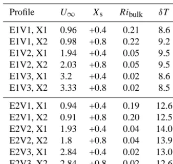
Table 1. Experimental setup for six atmospheric profiles with am-bient wind velocityV∞(m s−1), fetch distance over the snow patch
Xs (m), the bulk Richardson numberRibulk, and the temperature difference between the surface and the ambient air temperatureδT
(◦C). The labels of profiles refer to their position (X=Xs), ambient wind velocity (U=U∞), and the shape of the snow surface (flat: E1; concave: E2).
Profile U∞ Xs Ribulk δT
E1V1, X1 0.96 +0.4 0.21 8.6 E1V1, X2 0.98 +0.8 0.22 9.2 E1V2, X1 1.94 +0.4 0.05 9.5 E1V2, X2 2.03 +0.8 0.05 9.5
E1V3, X1 3.2 +0.4 0.02 8.6
E1V3, X2 3.33 +0.8 0.02 8.5
E2V1, X1 0.94 +0.4 0.19 12.6 E2V1, X2 0.91 +0.8 0.20 12.5 E2V2, X1 1.93 +0.4 0.04 14.0
E2V2, X2 1.8 +0.8 0.04 13.9
E2V3, X1 2.84 +0.4 0.02 13.0 E2V3, X2 2.84 +0.8 0.02 12.6
dimensions (zmax:l=0.06) were defined to scale with a cav-ity in the Wannengrat catchment (zmax:l=2.5:60=0.04), which was studied by Mott et al. (2013), revealing boundary-layer decoupling above a melting snowfield. We conducted our experiments on a manually designed concave depression made with compacted natural snow that was melting during the experiments. Much care was taken to ensure smooth tran-sition between the upstream fetch and the snow fetch as well as to construct a smooth concave section. The snowpack was isothermal during all experiments.
For experiments E1 and E2 profiles of mean and turbu-lent quantities were measured at 0.4 m (X1) and 0.8 m (X2) downwind of the leading edge of the snow patch. For E2, the depth of the snow-covered depression is 0.06 m at X1 and 0.1 m at X2. All experiments were performed at free-stream wind velocities of approximately 1, 2, and 3 m s−1 (V1, V2, and V3, respectively). All heights are given rela-tive to z=0, which is the height of the wooden floor and the initial snow cover at fetch distance 0. For the concave setup, z=0 corresponds to the highest point of the cavity. Consequently, for the concave setup E2 the snow surface be-longs toz= −0.06 m at X1 and toz= −0.1 m at X2. Please note that, due to the configuration of the probes, we were able to measure closer to the ground for the flat setup (E1) than for the concave setup (E2). While the lowest measure-ment point above snow is approximately 0.002 m for E1, it is 0.01 m for E2. Furthermore, the snow surface temperature was at its melting point during the whole experiment, result-ing in a change of the snow surface durresult-ing the experimental period. As a consequence of the melting snow surface, the heights above the snow surface are not consistent throughout
the experimental period. Thus, profiles not only of E2 but also of E1V2 and E1V3 feature negative heights.
The temperature and velocity fluctuations were mea-sured simultaneously using a system of a two-component platinum-coated hot-wire anemometer (TSI 1240-60) and a one-component cold-wire anemometer (Dantec 55P11). The calibration was performed in situ before each test against a calibrated miniature fan anemometer (Schiltknecht Mini-Air20) for the velocity measurements and against a digital thermometer (Labfacility Tempmaster-100). To ensure high statistical stationarity of the fluxes, we designed our experi-ments by sampling the flow at, at least, 100 times the integral timescale (Tropea et al., 2007). Data were acquired at a fre-quency of 1 kHz and for 100 s during the tests on setup 1 and 20 s during the tests on E2. The data were low-pass-filtered by means of a Butterworth filter with a cut-off frequency of 100 Hz. Furthermore, to eliminate low-frequency trends in the signal, data were also high-pass-filtered with a cut-off frequency of 0.2 Hz. With the tests being conducted at low velocities, a threshold was applied based on the Reynolds (the ratio of momentum forces to viscous forces) and Grashof number (the ratio of the buoyancy to viscous forces) to elimi-nate velocity data significantly influenced by natural convec-tion of the wire (Collis and Williams, 1958). The time series exceeding the latter threshold for more than 10 % of the time were not considered for the following analysis. Following this procedure four points in total have been removed from the data set. To account for the slope at measurement location X1, we applied the planar fit approach following Wilczak et al. (2001).
We estimated the uncertainty, considering both the system-atic and random components. The random uncertainty is sig-nificantly larger than the systematic uncertainty. The random uncertainty of a variableqwas considered as follows:
uq=σq/(hqi √
N , (1)
withσ being the standard deviationN being the number of independent samples separated by the integral timescale of
Figure 1. Sketch of the SLF boundary-layer wind tunnel and measurement setup of experiment 1 (flat setup, E1) and experiment 2 (concave setup, E2). Measurement positions X are given relative to the leading edge of the snow patch, with X0= −0.1 m, X1=0.4 m, and X2= 0.8 m. Note that all heightszused in the following figures are relative to the height of the topographical stepz=0. Consequently for the concave setup, the local surface at X1 corresponds toz= −0.06 m and at X2 toz= −0.1 m.
2.2 Quadrant analysis
Quadrant analysis consists of conditionally averaging the shear stresses into four quadrants depending on the sign of the stream-wise and vertical velocity fluctuations (Wallace et al., 1972).
Ifuandwcorrespond to stream-wise and vertical veloc-ity and primes indicate the deviation from the average value, each quadrant eventhu0w0i
i can be defined as
hu0w0ii= lim
T→∞ 1
T
T Z
0
u0(t )w0(t )Ii[u0(t )w0(t )]dt, (2)
whereT is the length of the time series andIi is a function
that triggers of a specific quadrantQi:
Ii[u0(t )w0(t )] = }1∀(u
0w0)∈Q
i
0∀(u0w0)6∈Q
i. (3)
The resulting types of motions are the following: outward motion of high-momentum fluid (quadrant 1), ejections of momentum fluid (quadrant 2), wallward motion of low-momentum fluid (quadrant 3), and sweeps of high-moment fluid towards the wall (quadrant 4). The four quadrants are defined as follows:
Quadrant 1 (Q1):u0>0, v0>0→(u0, v0)∈Q1,
Quadrant 2 (Q2):u0<0, v0>0→(u0, v0)∈Q2,
Quadrant 3 (Q3):u0<0, v0<0→(u0, v0)∈Q3,
Quadrant 3 (Q3):u0>0, v0<0→(u0, v0)∈Q4.
While Q1 and Q3 motions are positive stress-producing motions, ejections and sweeps contribute positively to the Reynolds stress. The negative contributions by Q1 and Q3 motions correspond to the interaction between ejection and sweep motions. In neutrally stratified boundary-layer flows, the main contributions to the Reynolds stress comes from sweep and ejection motions, and both motions are nearly equal (Wallace et al., 1972).
In our case all the events from each quadrant are consid-ered and no event is discarded based on its magnitude. There-fore the analysis concentrates on the overall flow dynamics rather than focusing on the strength of the motions. The sec-ond (ejections) and fourth (sweeps) quadrants constitute a positive contribution to the production of turbulent kinetic energy and to the momentum flux towards the surface, while the other two constitute a negative contribution.
3 Results
3.1 Experimental conditions
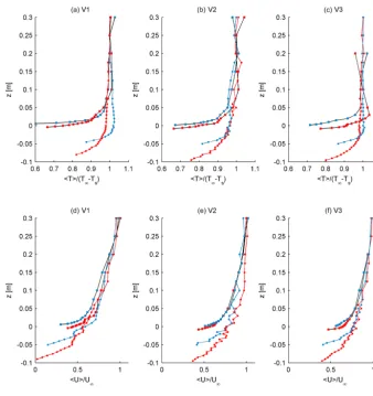
Figure 2. Vertical profiles of the mean air temperature (top) and wind velocity (bottom) normalized by the free-stream temperature/wind velocity.
the flow is expected to be dynamically unstable and turbu-lent. For both setups, the bulk Richardson number (Ribulk) was slightly higher at X2 than at X1 due to a slightly stronger cooling of the atmosphere further downwind. While the flow for the experimental cases with low free-stream wind (V1) was statically stable with Ribulk numbers ranging between 0.19 and 0.22, experimental cases driven by higher free-stream wind velocities (V2,V3) show low Ribulk numbers ranging between 0.02 and 0.05.
3.2 Vertical profiles of mean quantities
The vertical profiles of the stream-wise wind velocity U
and mean air temperatureT are illustrated in Fig. 2 for the different experimental cases and fetch distances. The mean air temperature is normalized by the difference between the ambient air temperatureT∞and the surface temperatureTs (which was 0◦C throughout the measurements). The mean wind velocityU is normalized by the free-stream wind ve-locityU∞.
The velocity profiles of E1 show a weakly pronounced lo-cal wind velocity maximum formed at X2 for low free-stream wind velocity (E1V1). For higher free-stream wind veloci-ties (E1V2, E1V3), the profiles exhibit a gradually increas-ing wind velocity with height without a local maximum ev-ident. The near-surface wind velocities are slightly higher at X2 than at X1. Wind profiles of E2 show a local wind maxi-mum for the low-wind-velocity case E2V1, which is less pro-nounced for E2V2. For the experiment with high free-stream wind velocities (E2V3), the formation of the local wind max-imum is not evident anymore. For E2V1, the wind profile at X1 shows a local wind maximum atz= −0.025 m (0.035 m above the local surface). At X2, the wind maximum was mea-sured at z= −0.05 m (which corresponds to 0.05 m above the local snow surface). The low-level maxima in velocity might be caused by the acceleration of the flow behind the topographical step (the highest point of the cavity) due to the detachment from the surface. A deep layer of strong wind velocity gradient is visible below the peak of wind velocity. Close to the wall, wind velocities become very small (smaller than 0.2 m s−1) and are much smaller for both distances than measured over the flat snow patch (E1) for a similar ambi-ent wind velocity. The extremely low values of wind veloci-ties within the cavity for the low-wind-velocity case indicates boundary-layer decoupling there. The temperature profiles for the low-wind-velocity cases are two-layered and show a change of temperature gradient at the height of the respective peaks in wind speed. Similar to the low-wind-velocity case, temperature profiles of the high-wind-velocity cases show a strong layering that coincides with the wind velocity profile.
3.3 Vertical profiles of turbulent quantities
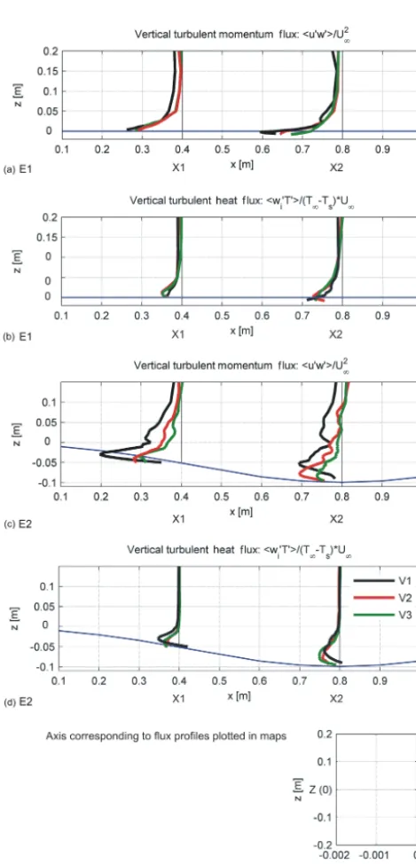
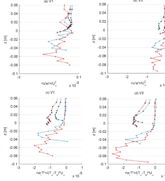
Figure 3 illustrates vertical profiles of turbulent momentum flux and vertical turbulent heat flux along the snow patch for the flat and the concave setup. Fluxes are normalized by the free-stream wind velocity and temperature difference be-tween snow surface and ambient air. Figure 4 zooms in on the near-surface profiles (ranging fromz= −0.1 to + 0.06 m) of turbulent momentum and vertical turbulent heat flux for the low-wind-velocity case V1 and the high-wind-velocity case V3. Primes indicate the deviation from the mean value, and overbars the average. Momentum fluxes are thus computed as a covariance between instantaneous deviation in horizon-tal wind speed (u0) from the mean value (u) and instanta-neous deviation in vertical wind speed (w0) from the mean value (w). Vertical heat fluxes are computed as a covariance between instantaneous deviation in air temperature (T0) from the mean value (T) and instantaneous deviation in vertical wind speed (w0) from the mean value (w). In theory a ther-mal internal boundary layer develops with increasing depth in downwind distance as a neutrally stratified flow crosses a single snow patch. Assuming that all measurements are con-ducted above the roughness sublayer, turbulent momentum and vertical turbulent heat fluxes within the stable internal
boundary layer are expected to increase with decreasing dis-tance to the snow surface (Essery et al., 2006).
For experiments conducted over the flat snow patch E1, profiles reveal an increase of negative momentum fluxes with decreasing distance to the snow surface (Figs. 3a, 4a, c). Con-trarily, the vertical profiles of turbulent quantities for the con-cave snow patch (Figs. 3c, 4a, c) show a distinct maximum in the negative vertical momentum flux at the height of the shear layer, indicating that both the surface and the high-shear region aroundz=0 contribute to turbulence genera-tion. For low wind velocities, profiles of momentum fluxes feature a distinct peak approximately 0.03–0.04 m above the local surface for X1 and X2 (Figs. 3c, 4a, c). Below that max-imum, momentum fluxes strongly decrease towards the snow surface. This near-surface suppression of momentum flux is strongest further downwind at X2, at the maximum depth of the cavity. The peak of the momentum flux appears to be strongest at the first measurement location downstream of the fetch transition (X1). At the downwind location X2, however, the magnitude of the momentum flux is much lower for the whole profile.
At X1, profiles of the vertical turbulent heat flux reveal a local maximum at z= +0.02 m for the flat snow patch with a decrease towards the surface below that maximum (Figs. 3b and 4c, d). Further downwind, the maximum heat flux was measured at the lowest point above the surface (z= +0.002 m), and no suppression of the vertical turbulent heat flux was measured there. On the contrary, for the concave setup, all profiles of heat fluxes feature a similar shape re-vealing distinct peaks of fluxes at the lowest few centimeters of the atmospheric layer (0.02–0.04 m above the local sur-face), coinciding with the maximum in vertical velocity fluc-tuations (not shown). Below that maximum, fluxes strongly decrease towards the snow surface (Figs. 3d and 4). The max-imum can be found at a higher distance to the ground for the low-wind-velocity case E2V1, coinciding with maximum wind speed at a height of 0.04–0.05 m above the local snow surface and strong shear below the local wind maximum (Figs. 2, 4). Close to the surface, the fluctuation of stream-wise and vertical velocity fluctuations are rapidly suppressed at both downwind distances and for all wind velocities. For higher wind velocities, however, the suppression of the ver-tical heat flux is confined to the lowest 0.01–0.02 m of the ABL and is much stronger for the downwind distance X2, where the maximum depth of the cavity is reached (Fig. 4d).
3.4 Turbulence phenomena at the snow surface
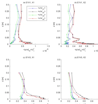
Results from the quadrant analysis are presented for the flat setup E1 (Fig. 5) and the concave setup E2 (Fig. 6). The stress fraction contribution of each quadrant gives insight into the physics of turbulence structures close to the wall (snow cover).
Figure 3. Vertical profiles of the turbulent fluxes: momentum flux u0w0and turbulent vertical heat fluxw0T0normalized by the tem-perature difference and free-stream wind velocity, plotted at the cor-responding measurement location along the snow patch for the flat and concave setups. The axis corresponding to the flux profiles is plotted outside of the individual plots.
stress comes from sweep and ejection motions, and both mo-tions are nearly equal in their contribution (Wallace et al., 1972). In the following, we will discuss the near-surface pro-files resulting from our experiments with flows characterized by a changing atmospheric stability towards the surface. We particularly want to distinguish between turbulence phenom-ena observed for the flat and the concave setup. For E1 the ejections (Q2) and sweeps (Q4) are observed to dominate the other two events over the whole boundary-layer depth (Fig. 5). Both contributions increase with decreasing distance to the wall, promoting the downward-directed momentum flux. This result is consistent for all free-stream wind veloci-ties (i.e., experiments E1V1, E1V2, E1V3). This distribution is analogous to the distribution of quadrant motions in neu-trally stratified boundary-layer flows over flat surfaces, where the ejection–sweep cycle was observed to be induced by co-herent flow structures (Adrian et al., 2000).
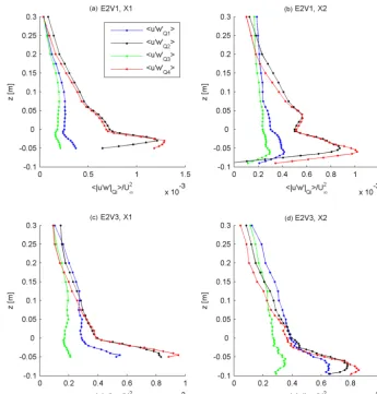
Over the concave snow patch E2, ejections and sweeps are observed to dominate over the other two quadrant motions, similarly to the flat case (Fig. 6). In contrast to E1, profiles for E2 reveal a clear dominance of sweeps (Q4) of high-speed fluid directed downward close to the snow surface for all se-tups, in particular for the lowest-wind-velocity case E2V1, where larger stability is also observed (Fig. 6). This marks a clear difference with the distribution of quadrant events for boundary-layer flows in neutral-stability conditions (see Methods section). At the lowest velocity it is interesting to observe that the peak of both ejections (Q2) and sweeps (Q4) (i.e., the height of peak wind velocity) occurs at a signifi-cantly higher distance from the snow surface than in the case of the two other tests at higher velocity. The strong suppres-sion of turbulent motions close to the surface is a clear indi-cation for boundary-layer decoupling at low wind velocities and will be discussed in the following section.
4 Discussion: indications of boundary-layer decoupling within the cavity
In order to discuss the near-surface turbulence in more de-tail, we show the near-surface profiles of mean wind veloc-ity, the vertical momentum, and heat fluxes, as well as the shear stress distribution for the low- and high-wind-velocity cases at the different measurement locations (Fig. 7). Fig-ure 8 shows the gradient Richardson number calculated from local wind and temperature gradients for atmospheric layers (height of layers is 0.025 m) and the Reynolds number calcu-lated from the local wind velocity at the respective measure-ment point for experimeasure-ments E2V1 and E2V3.
Figure 4. Vertical profiles of the turbulent fluxes: momentum fluxu0w0(a, b) and vertical heat fluxw0T0(c, d) normalized by the temperature difference and free-stream wind velocity.
of the local wind maximum (Fig. 7f, g). The region below this local flow acceleration corresponds to a region of re-duced turbulent mixing as observed in the vertical profiles of heat and momentum flux (Fig. 7f, g). The rapid decrease of all strong local motions below the peak atz= −0.05 m fur-ther confirms a strong suppression of turbulent mixing, thus strong atmospheric decoupling over the deepest point of the concave. Boundary-layer decoupling is also revealed by the high gradient Richardson numbers for those points within the cavity, clearly exceeding the critical value of 0.25 only for the low-wind-velocity case (Fig. 8a). Furthermore, very low Reynolds numbers calculated for measurement points below
z= −0.05 m that are significantly lower than for the higher-wind-velocity case indicate laminar flow close to the surface (Fig. 8b). These profiles suggest that the higher stability at X2 at the lowest velocity forces the unsteady and coherent flow structures to develop above the cold pool. Moreover, in this latter case such strong reduction of ejections (Q2) and sweeps (Q4) in the decoupled region to the level of the other
two quadrant events causes the vertical momentum flux to reduce toward zero (Fig. 7f). The strong suppression of high-momentum fluid from the outer region and the strong sup-pression of turbulent mixing close to the wall (Fig. 8) in-dicates favorable conditions for cold-air pooling within the cavity, which is strongest at the maximum depth of the cav-ity (Fig. 7f, g).
Figure 5. Shear stress contribution of the quadrants for the experimental setups E1V1 and E1V3.
values close to the wall. This strong increase of outward interactions (Q1) which are observed to increase with the free-stream velocity (Fig. 7l, p) is a further clear departure from the commonly observed distribution of quadrant mo-tions in neutrally stratified boundary-layer flows. The posi-tive stream-wise fluctuations, given by the Q1 and Q4 events, dominate the flow especially at the highest free-stream veloc-ities (Fig. 7p). This is due to sweeps (Q4) towards the near-surface region as discussed above and to the resulting dis-placement of high-speed, colder fluid upwards (Q1) from the near-surface region as an effect of the stronger mixing occur-ring at the higher velocities. The outward interactions (Q1) can therefore be seen as bouncing flow resulting from pre-ceding sweeps (Q4) directed towards the snow surface. This finds confirmation in the observation at the higher tested free-stream velocity E2V3 where the sweeps (Q4) peak closer to the snow surface, and in the relatively higher outward inter-actions (Q1) at X2 where the concave section allows the cold pool to form and as a consequence the mixing process to be stronger at the highest velocities. Thus, the inertial forces
ap-pear to be strong enough to mix most of the boundary layer within the cavity, causing an enhancement of turbulent fluxes of momentum and heat close to the wall. At the deepest point of the cavity, however, the turbulent mixing is still suppressed within a very shallow layer at the wall, and the concave sur-face still allows cold-air pooling.
con-Figure 6. Shear stress contribution of the quadrants for the experimental setups E2V1 and E2V3.
ditions and within sheltered locations, when buoyancy effects start to dominate over turbulence generation by shear. Thus, for typical melt conditions of a seasonal snow cover, only the special experimental conditions with a concave-shaped snow patch and low free-stream wind velocities allowed the de-velopment of near-surface vertical profiles of turbulence that are typical for very stable regimes (Mahrt, 2014) when the maxima of turbulence is reached in a layer decoupled from the surface. For high free-stream wind velocities, the iner-tia of the flow becomes strong enough to mix the boundary layer above the snow surface (also for concave setup) and to consequently inhibit the stagnation of cold air and associated boundary-layer decoupling within the local depression.
The general requirements of the experimental design, us-ing natural snow for our experiments and performus-ing all experiments for typical spring conditions (air temperatures above 5◦C), strongly restricted the time of year when experi-ments could be run. In summary, repeating the measureexperi-ments had the following limitations:
– Measurements could be only performed during typical spring conditions: when natural snow has been available and temperatures are clearly above the melting point but also not too high to create untypically stable conditions. – All measurements had to be finished within 1 day and within a few hours of that day when air temperatures were high enough during daytime.
– The snow cover was melting, and we had to prepare the snow cover for each single experimental design. Al-though the procedure we adopted to design the concave section filled with compacted snow allowed the con-struction with sufficient precision, rebuilding the sec-tion for each experimental run might have result in a significant increase of the measurement uncertainty due to small differences in the surface characteristics (see uncertainty estimates in the Supplement).
Figure 7. Near-surface vertical profiles of mean wind speed, turbulent momentum flux, turbulent heat flux, and shear stress distribution over the concave snow patch for experiment E2V1 at measurement locations X1 (a–d) and X2 (e–h), and for experiment E2V3 at X1 (i–l) and at X2 (m–p). Red horizontal lines mark the area of local wind maxima. Horizontal black lines indicate the upper limit of the near-surface suppression of turbulence. The black double arrow marks the layer where near-surface turbulence appears to occur.
varying footprints for the fluxes depending on wind speeds. At the same time, the differences between profiles at X1 and X2 give a first indication of how fluxes change in the stream-wise direction. It is clear that lateral transport of heat and mo-mentum plays an important role for the given conditions and
that the net effect of a topographic depression on the bound-ary layer above still needs to be systematically analyzed.
Figure 8. Vertical profiles of the (a) gradient Richardson numberRigcalculated from temperature and wind velocity gradients over a layer of dz=0.025 m and (b) Reynolds numberRecalculated from the local wind velocity at each measurement point.
wind conditions indicating boundary-layer decoupling. The measurements of Mott et al. (2013) were, however, only con-ducted over a concave-shaped snow patch and lacked simul-taneous measurements over a flat snow patch. Furthermore, measurements of the vertical profiles of turbulence intensi-ties that were conducted by a eddy-correlation system were restricted by the low possible number of three measurement points. Compared to field measurements, the experimental setup in the wind tunnel allowed a high vertical resolution of flux measurements and allowed us to account for the effect of the topography on the flow development and the generation of turbulence in the atmospheric layer adjacent to the snow. Comparing wind tunnel with field experiments, we have to consider that in the field other meteorological processes such as radiation may also become important drivers for cold-air pooling and boundary-layer decoupling. We expect, however, that these effects are extremely small over the length scales of our wind tunnel.
5 Conclusions
Wind tunnel experiments on flow development over a melt-ing snow patch were conducted for meteorological condi-tions typically observed over patchy snow covers and strong snow melt in alpine environments. For the first time wind tunnel experiments were conducted over a snowfield to ex-plore the relative role of topography versus pure thermody-namics in causing atmospheric decoupling for melting snow conditions. The experiments give evidence that topography is critical for the process of atmospheric decoupling by signif-icantly altering the near-surface flow field due to sheltering
effects. While the stability had only a small effect on flow dynamics over the flat snowfield, it strongly influenced the near-surface flow behavior over the concave-shaped snow patch, especially if the free-stream wind velocity was low. For that experimental setup, the near-surface suppression of turbulence was observed to be strongest, and the high-speed fluid was decoupled from the surface, enhancing atmospheric stability close to the surface and promoting the cold-air pool-ing over the spool-ingle snow patch. The atmospheric decouplpool-ing was clearly revealed by flux profile measurements (strong suppression of momentum and heat fluxes) and by quadrant analysis (strong reduction of ejections and sweeps in the de-coupled region). At higher wind velocities, the strongest tur-bulent mixing was measured much closer to the surface, in-dicating a rush-in of high-momentum fluid of the outer layer to the wall region. Below the wind maximum, however, a very shallow layer characterized by a suppression of turbu-lent mixing was still present. Over the flat snow patch, pro-files with low free-stream wind speeds only involved a weak suppression of the turbulent mixing in a very shallow layer above the snow cover. Thus, the strong atmospheric decou-pling and cold-air pooling over single snow patches appear to be promoted by the cooling effect of the snow in sheltered locations, causing the local development of a very stable in-ternal boundary layer above the snow patch.
the survival of long-lasting snow patches or all-season snow and ice fields in alpine or cold environments. The quantita-tive contribution of the atmospheric decoupling over melt-ing snow for the total mass and energy balance of a com-plete alpine catchment is not yet known. Although first nu-merical results of Mott et al. (2015) show that the interac-tion between boundary-layer flow and fracinterac-tional snow cover significantly affects the total energy balance, field measure-ments conducted over a larger area and for a complete melt season are necessary to estimate the relative frequency of phenomena enhancing (advective heat transport) or slowing down (atmospheric decoupling) snow melt. Such a compre-hensive experimental study is currently being conducted in a three-years project in an alpine catchment in the Swiss Alps. Extensive field experiments during the entire ablation period are expected to provide new insight into the frequency of de-scribed phenomena and the importance for the snow hydrol-ogy of the total catchment.
The Supplement related to this article is available online at doi:10.5194/tc-10-445-2016-supplement.
Acknowledgements. The work presented here is mainly supported
by the Swiss National Science Foundation SNF, financing the instrumentation (grants 206021_133786 and 200020-112022), the wind tunnel facility (grant 2160-060998) and projects supporting the experiments (grants 200021_150146 and 200021_147184).
Edited by: M. van den Broeke
References
Adrian, R. J., Meinhart, C. D., and Tomkins, C. D.: Vortex organi-zation in the outer region of the turbulent boundary layer, J. Fluid Mech., 422, 1–54, 2000.
Bodine, D., Klein, P., Arms, S., and Shapiro, A.: Variability of sur-face air temperature over gently sloped terrain, J. Appl. Meteo-rol., 48, 1117–1141, 2009.
Burns, P. and Chemel, C.: Evolution of Cold-Air-Pooling Pro-cesses in Complex Terrain, Bound.-Lay. Meteorol., 150, 423– 447, doi:10.1007/s10546-013-9885-z, 2014.
Collis, D. C. and Williams, M. J.: Two-domensional convection from heated wires at low Reynolds numbers, J. Fluid Mech., 6, 357–384, doi:10.1017/S0022112059000696, 1959.
Dadic, R., Mott, R., Lehning, M., and Burlando, P.: Wind Influence on Snow Depth Distribution and Accumulation over Glaciers, J. Geophys. Res., 115, F01012, doi:10.1029/2009JF001261, 2010. Essery, R.: Modelling fluxes of momentum, sensible heat and latent heat over heterogeneous snowcover, Q. J. Roy. Meteor. Soc., 123, 1867–1883, 1997.
Essery, R., Granger, R., and Pomeroy, J. W.: Boundary-layer growth and advection of heat over snow and soil patches: modelling and parameterization, Hydrol. Process., 20, 953–967, 2006.
Fujita, K., Hiyama, K., Iida, H., and Ageta, Y.: Self-regulated fluc-tuations in the ablation of a snow patch over four decades, Water Resour. Res., 46, W11541, doi:10.1029/2009WR008383, 2010. Granger, R. J., Pomeroy, J. W., and Essery, R.: Boundary-layer
growth and advection of heat over snow and soil patches: field observations, Hydrol. Process., 20, 953–967, 2006.
Gustavsson, T., Karlsson, M., Bogren, J., Lindqvist, S.: Develop-ment of temperature patterns during clear nights, J. Appl. Mete-orol., 37, 559–571, 1998.
Lehning, M., Löwe, H., Ryser, M., and Raderschall, N.: Inhomogeneous precipitation distribution and snow trans-port in steep terrain, Water Resour. Res., 44, W09425, doi:10.1029/2007WR006544, 2008.
Liston, G. E.: Local advection of momentum, heat and moisture during the melt of patchy snow covers, J. Appl. Meteorol., 34, 1705–1715, 1995.
Mahrt, L.: Stably stratified atmospheric boundary layers, Annu. Rev. Fluid Mech., 46, 23–45, 2014.
Mann, J. and Lenschow, D. H.: Errors in airborne flux measurements, J. Geophys. Res., 99, 14519–14526, doi:10.1029/94JD00737, 1994.
Mott, R., Schirmer, M., Bavay, M., Grünewald, T., and Lehning, M.: Understanding snow-transport processes shaping the mountain snow-cover, The Cryosphere, 4, 545–559, doi:10.5194/tc-4-545-2010, 2010.
Mott, R., Egli, L., Grünewald, T., Dawes, N., Manes, C., Bavay, M., and Lehning, M.: Micrometeorological processes driving snow ablation in an Alpine catchment, The Cryosphere, 5, 1083–1098, doi:10.5194/tc-5-1083-2011, 2011.
Mott, R., Gromke, C., Grünewald, T., and Lehning, M.: Relative im-portance of advective heat transport and boundary layer decou-pling in the melt dynamics of a patchy snow cover, Adv. Water Resour., 55, 88–97, doi:10.1016/j.advwatres.2012.03.001, 2013. Mott, R., Scipión, D. E., Schneebeli, M., Dawes, N., and Lehn-ing, M.: Orographic effects on snow deposition patterns in mountainous terrain, J. Geophys. Res.-Atmos., 119, 1419–1439, doi:10.1002/2013JD019880, 2014.
Mott, R., Daniels, M., and Lehning, M.: Atmospheric flow develop-ment and associated changes in turbulent sensible heat flux over a patchy mountain snow cover, J. Hydrometeorol., 16, 1315–1340, doi:10.1175/JHM-D-14-0036.1, 2015.
Neumann, N. and Marsh, P.: Local advection of sensible heat in the snowmalt landscape of Arctic tubdra, Hydrol. Process., 12, 1547–1560, 1998.
Ohya, Y.: Wind-Tunnel Study Of Atmospheric Stable Boundary Layers Over A Rough Surface, Bound.-Lay. Meteorol., 98, 57– 82, doi:10.1023/A:1018767829067, 2001.
Ohya, Y.: Intermittent bursting of turbulence in a stable boundary layer with low-level jet, Bound.-Lay. Meteorol., 126, 349–363, doi:10.1007/s10546-007-9245-y, 2008.
Price, J. D., Vosper, S., Brown, A., Ross, A., Clark, P., Davies, F., Horlacher, V., Claxton, B., McGregor, J. R., Hoare, J. S., Jemmett-Smith, B., and Sheridan, P.: COLPEX: field and numer-ical studies over a region of small hills, B. Am. Meteorol. Soc., 92, 1636–1650, 2011.
Tropea, C., Yarin, A. L., and Foss, J. F. (Eds.): Springer handbook of experimental fluid mechanics, Springer Science & Business Media, 2007.
Vosper, S. B., Hughes, J. K., Lock, A. P., Sheridan, P. F., Ross, A. N., Jemmett-Smith, B., and Brown, A. R.: Cold-pool forma-tion in a narrow valley, Q. J. Roy. Meteorol. Soc., 140, 699–714, doi:10.1002/qj.2160, 2014.
Whiteman, C. D., Zhong, S., Shaw, W. J., Hubbe, J. M., Bian, X., and Mittelstadt, J.: Cold pools in the Columbia basin, Weather Forecast., 16, 432–447, 2001.
Whiteman, C. D., Muschinski, A., Zhong, S., Fritts, D., Hoch, S. W., Hahnenberger, M., Yao, W., Hohreiter, V., Behn, M., Cheon, Y., Clements, C. B., Horst, T. W., Brown, W. O. J., and Oncley, S. P.: METCRAX: Meteorological experiments in Arizonas Meteor Crater, B. Am. Meteor. Soc., 89, 1665–1680, 2008.
Wallace, J. M., Eckelmann, H., and Brodkey, R. S.: The wall region in turbulent shear flow, J. Fluid Mech., 54, 39–48, 1972. Wilczak, J., Oncley, S., and Stage, S.: Sonic Anemometer Tilt
Correction Algorithms, Bound.-Lay. Meteorol., 99, 127–150, doi:10.1023/A:1018966204465, 2001.