Extreme event return times in long-term memory processes near 1/f

(1)

www.nonlin-processes-geophys.net/15/557/2008/ © Author(s) 2008. This work is distributed under the Creative Commons Attribution 3.0 License.

Nonlinear Processes

in Geophysics

Extreme event return times in long-term memory processes near 1

/f

R. Blender, K. Fraedrich, and F. Sienz

Universit¨at Hamburg, Meteorologisches Institut, Bundesstrasse 55, 20146 Hamburg, Germany

Received: 2 August 2007 – Revised: 17 June 2008 – Accepted: 17 June 2008 – Published: 16 July 2008

Abstract. The distribution of extreme event return times and their correlations are analyzed in observed and simu-lated long-term memory (LTM) time series with 1/f power spectra. The analysis is based on tropical temperature and mixing ratio (specific humidity) time series from TOGA COARE with 1 min resolution and an approximate 1/f

power spectrum. Extreme events are determined by Peak-Over-Threshold (POT) crossing. The Weibull distribution represents a reasonable fit to the return time distributions while the power-law predicted by the stretched exponential for 1/f deviates considerably.

For a comparison and an analysis of the return time pre-dictability, a very long simulated time series with an approx-imate 1/fspectrum is produced by a fractionally differenced (FD) process. This simulated data confirms the Weibull dis-tribution (a power law can be excluded). The return time se-quences show distinctly weaker long-term correlations than the original time series (correlation exponentγ¯≈0.56).

1 Introduction

Long-term memory (LTM) is a ubiquitous phenomenon in natural time series and mainly identified by power-laws char-acterized by a single correlation exponentγ in the correla-tion funccorrela-tion,C(t )∼t−γ (Fraedrich and Blender, 2003). In many observed time series, predominantly sea surface tem-peratures, 1/f power spectra are found related to smallγ

(Weissman, 1988; Monetti et al., 2003). In the current dis-cussion on anthropogenic climate change, the simulation of LTM becomes relevant since anthropogenic trends may be masked by low frequency internal variability (Blender and Fraedrich, 2003).

Correspondence to: R. Blender ([email protected])

Even weak LTM (with γ slightly below 1) has consid-erable impacts on return times of extreme events (Altmann and Kantz, 2005; Eichner et al., 2007). An obvious reason for this effect is the clustering of threshold crossings dur-ing periods with high averages (Bunde et al., 2005). The distribution of return timestr in the presence of LTM is

ap-proximately given by a stretched exponential,p∼exp(−trγ),

where the exponent is assumed to be identical to the corre-lation exponent γ. The stretched exponential is motivated by the study of Newell and Rosenblatt (1962) who derived an upper bound for the probability of no zero crossings in power-law correlated Gaussian processes. Olla (2007) ap-plied an-expansion for γ=1− and obtained a stretched exponential distribution with exponent γ. Stretched expo-nential distributions are found for linear systems with LTM (Altmann and Kantz, 2005). There are classes of nonlinear dynamical systems which show algebraic (power-law) dis-tributions (Zaslavsky, 2002). For inter-event disdis-tributions of earth quakes Corral (2004) suggests a gamma distribution. The long-term memory does not only alter the distribution of return times but also their temporal correlations which are the basis for the return time predictability (Bunde et al., 2004; Altmann and Kantz, 2005).

(2)

558 R. Blender et al.: Extreme event return times The paper is organized as follows: In Sect. 2 LTM is

de-fined and available results on return time distributions are summarized. The long term memory properties and the re-turn time distributions of the observational data are deter-mined in Sect. 3. In Sect. 4 simulated time series are com-pared and the correlation properties of the extreme event in-tervals are analyzed. The Sect. 5 concludes with a summary and discussion.

2 Estimating long-term memory and extreme event re-turn time statistics

For the estimation of long-term memory (LTM, Beran, 1994) several methods are available. We compare results of the De-trended Fluctuation Analysis (DFA, Peng et al., 1994) with fits of FARIMA (p, d,0) processes (Hosking, 1981). The FARIMA processes are able to assess the contributions of short- and long-term components. The distribution of the ex-treme event return times is altered in the presence of LTM since long periods with anomalous low or high persistent de-viations occur. The correlations between successive extreme event return times are useful for the prediction of extreme event return times.

2.1 Long-term memory analysis

A time series has long-term memory (LTM, also denoted as long-term persistence) if the correlation functionC(t )is not integrable (Beran, 1994). For a long-term power-law decay,

C(t )∼t−γ, LTM is equivalent toγ >0. Empirical time series have LTM if the autocorrelation follows a power-law with exponent 0<γ <1 for the largest time scales present. LTM is ubiquitous in nature and shows up mainly in temperature records (Fraedrich and Blender, 2003; Huybers and Curry, 2006). The exponentβof the power spectrum,S(f )∼f−β, and the correlation exponent are related byβ=1−γ, hence the power spectrum increases with decreasing frequency for

γ <1.

To determine LTM properties two methods are applied (see Sect. 2.1): Detrended fluctuation analysis (DFA, Peng et al., 1994), and an estimation of the parameters in FARIMA (p, d,0) processes (Hosking, 1981).

The two methods are independent complements for the analysis of our data and inhibit an erroneous detection of LTM: While there is a known LTM detection problem in the DFA in short term memory time series (Maraun et al., 2004), this method does not require any model assumption (for ex-ample normality of the data). The FARIMA process is ideal for the detection of short- and long-term memory, in addi-tion, it allows a significance test for the number of parame-ters, however, normality of the data is required.

(i) The DFA determines fluctuationsF (τ )on time scalesτ

in stationary anomaly sequences with LTM. Trends in the time series can be eliminated by extensions of the DFA (Fraedrich and Blender, 2003).

(ii) To assess the contributions of short- and long term memory components, fits of autoregressive processes (AR) and fractionally integrated autoregressive process are considered. In the following, FAR is used as a short notation for FARIMA (p, d,0) (Hosking, 1981) which includes an autoregressive (AR) process of orderpand a fractionally differenced (FD) process with dimension

d.

The AR process is defined by

φ (B)xt =t (1)

whereBis the backshift operator defined byBxt=xt−1, and

t is white noise. Using the coefficientsan, the polynomial φ (B)is

φ (B)xt =xt− p

X

n=1

anxt−n (2)

The FD process (Hosking, 1981) is derived from

(1−B)dxt =t (3)

and leads to an AR process of infinite order

xt = ∞ X

n=1

anxt−n+t, an= −

0(n−d)

0(−d)0(n+1) (4)

For low frequencies the FD process shows a scaling power spectrumS(f )∼f−β with spectral exponentβ=2dand cor-relation exponentγ=1−2d.

The FAR process is given by the combination

φ (B)(1−B)dxt =t (5)

and is determined bypcoefficients in the AR and the dimen-siond.

2.2 Extreme event return distributions

An extreme event in a time series xi, i=1, . . . , N, crosses

a given thresholdq withxi>q. The return timetr between

two extreme events is the time interval between two events withxi>q andxi+tr>qand lower valuesxj<q in between, i<j <i+tr. The mean return timeRqdepends on the

thresh-old q and is approximated by the probability distribution function (pdf)D(x)of the time series

R_q−1= Z ∞

q

D(x)dx (6)

In the present paper, the thresholdqis determined to obtain a specific value ofRq. For uncorrelated data, the return times

are exponentially distributed following a Poisson process

pq(tr)=

1

Rq

exp(−tr/Rq) (7)

(3)

LTM leads to periods with anomalous persistent low or high deviations. During such periods extreme high values are ei-ther rare (for low anomalies) or frequent (during high anoma-lies). Thus return time statistics shows clustering which is not observed in time series without memory.

For LTM time series stretched exponential return time dis-tributions are suggested (Bunde et al., 2004; Altmann and Kantz, 2005; Eichner et al., 2007)

pq(tr)≈ aγ Rq

exp[−(bγtr/Rq)γ] (8)

Note that the scaling exponentγ is conjectured to be equal to the correlation exponent which characterizes LTM. The co-efficientsaγ=γ 0(2/γ )/ 02(1/γ )andbγ=0(2/γ )/ 0(1/γ )

are determined by normalisation ofpqand the condition for the mean,Rq=<tr>;0is the gamma-function.

In the limitγ→0, the stretched exponential approaches a power law

logpq(tr)∼ −slogtr +const (9)

with the exponent

s= lim

γ→0γ b

γ

γ =1.5 (10)

Altmann and Kantz (2005) and Eichner et al. (2007) con-sider the correlation exponents 0.05<γ <1 that is, between almost 1/f and white noise. Eichner et al. (2007) show that the stretched exponential is valid for several types of distri-butionsD.

For small return times,trRq, the observed distribution deviates from the stretched exponential (8) and scales as (see Eq. (10) in Eichner et al., 2007).

Rqpq(tr)∼

_tr

Rq

s0

(11) with the proposed values0=γ0−1,γ0≈γ for Gaussian den-sity. For large return times (trRq) the limit of the distribu-tion (8) is

Rqpq(tr)∼exp[−(btr/Rq)γ] (12)

The stretched exponential is accepted as an approximate rep-resentation for linear LTM processes (Altmann and Kantz, 2005; Eichner et al., 2007).

An alternative to the stretched exponential distribution (8) is the Weibull distribution (Sornette, 2006; Abaimov et al., 2007) with the scale parameterτ and the shape parameterγ

pW(tr)= γ τ

_t

r τ

γ−1

exp[−(tr/τ )γ] (13)

Note that the Weibull distribution forγ <1 is frequently de-noted stretched exponential distribution; this, however, dif-fers from (8) by the prefactor ∼tγ−1. Without reference to Weibull, the power-law (11) is suggested by Eichner et

al. (2007) in their Eq. (10) to correct the pure stretched expo-nential,∼exp(−tγ), for small return times.

The advantages of the Weibull distribution for the charac-terization of extreme event return times are:

(i) The Weibull distribution (13) combines (8) and the short time limit (11) and describes the observed distribution in a wide range of return times.

(ii) The cumulative distribution function is known,

FW(tr)=1−exp[−(tr/τ )γ], and the mean recurrence time is determined byR=τ 0(1+1/γ ). This cumulative distribution function is useful for statistical analyses. (iii) According to Sornette (2006) power-laws can be

ap-proximated by the Weibull distribution in arbitrary in-tervals to any prescribed accuracy.

The fit of the discrete power-law and Weibull distribution to the return time series is performed following Clausset et al. (2007). The approach fits the parameters of the distribu-tions (exponents for power-laws; shape and scale parameters for Weibull) using Maximum Likelihood estimation and de-termines an optimal range (restricted by a minimum return time cutoff) by minimizing the Kolmogorov-Smirnov dis-tance.

The correlations between successive extreme event return times are one of the most useful aspects in practical ap-plications of extreme value theory. Given time series with weak LTM (correlation exponentsγ=0.4 and 0.7), Bunde et al. (2004) analyse the respective return times arranged in a sequence, and find their long-term correlation exponentsγ

to be similar to the exponents of the original time series. It is expected that this relationship changes distinctly for very strong LTM due to its close vicinity to the nonstationarity threshold 1/f.

In this paper, extreme events are determined by the Peak-Over-Threshold (POT) method with different thresholdsq, which are adjusted for mean return times Rq. The

de-trended fluctuation analysis (DFA) is employed to determine the LTM of the observational data and the recurrence times in the simulated data. Fits of FARIMA process support the LTM analysis of observational data. The time series are sim-ulated by fractionally differenced processes (FD, Hosking, 1981). The fits of the power-law and the Weibull distribu-tions are performed by the code available from Clausset et al. (2007). For all other calculations we use the statistics software R (R Development Core Team, 2005).

3 High resolution observational data

(4)

560 R. Blender et al.: Extreme event return times and Lukas, 1992). The aim of the international field

ex-periment TOGA COARE during 1992–1993 was to study the atmospheric and oceanic processes over the western Pa-cific. The data measured at the Research Vessel (R/V) Kexue (3.9◦S, 155.9◦E) encompasses boundary layer near surface air temperature and the mixing ratio with one minute resolu-tion (Fig. 1); this data set has been corrected by Lucas and Zipser (2000). In the air temperature time series the diurnal cycle (daily mean with 1 min resolution) is removed for the analysis. The weak diurnal cycle in the mixing ratio is not removed since this does not change the result.

The mixing ratio (Fig. 1c) reveals the presence of a large scale event during the first part of the time series (due to a passing 40-day wave). The fluctuations of the temperature and the mixing ratio are characterized by a 1/f power spec-trum in a wide range of time scales (Yano et al., 2001, 2004). Only a part of this time series (8.8·104time steps, roughly 61 days) is analyzed to keep the number of missing values be-low<5%. The missing values are replaced by the mean and no attempt has been made to determine the effect of these replacements.

The overall behaviour of the data indicates nonstationar-ities in both time series. The frequency distributions for both time series (Fig. 1b, d) show deviations from Gaussian, which are, however, not substantial and presumably related to the nonstationarity.

3.1 Long term memory analysis

To determine LTM properties of the two observed time se-ries two methods are applied (see Sect. 2.1): Detrended fluc-tuation analysis (DFA, Peng et al., 1994), and an estimation of the parameters in FARIMA (p, d,0) process (Hosking, 1981).

(i) The DFA spectra in Fig. 2a, b show scaling fluctu-ation spectra, F (τ )∼τα, with exponents α≈1. . .1.1 close to a 1/f−spectrum (α=1) for the temperature and the mixing ratio. The power spectrum is closely related to F (τ ) and scales as S(f )∼f−β with expo-nentsβ=2α−1≈1. . .1.2; the correlation exponents are

γ=1−β≈0. . .−0.2. Note that the temperature fluctua-tion spectrum in Fig. 2a approachesα≈1 (γ=0) for long time periods (tr>103min) during two decades. An

anal-ysis of a trend-eliminating version of the DFA yields the same exponents.

(ii) Short- and long term memory contributions are assessed by fits of autoregressive processes (AR) and fractionally integrated autoregressive process (FAR); see Sect. 2.1. To determine the optimal number of parameters in the FAR fit, the Akaike information criterion (AIC) is used based on the minimum of

AIC= −2 log(L)+2k (14)

whereLis the maximized likelihood function andkthe number of estimated parameters. For temperature and mixing ratio it appears that the FAR process is supe-rior to AR processes for small numbers of coefficients (Fig. 3a,b). The mixing ratio shows a higher preference for the FAR than temperature, which can be explained by the higher degree of scaling (Fig. 2b). Furthermore, a maximum likelihood ratio test (99% significance) sup-ports a lower degree of the autoregressive component in the FAR for the mixing ratio.

Likelihood ratio tests are performed to test whether higher order models give significant improvement compared to lower order models. FAR-models are tested against all (AR and FAR) lower order models, while the test for the AR-models is only performed for lower order. Filled symbols (Fig. 3) show significance against lower order models on the 99% significance level.

For both observed datasets FAR-models outperform the ARs for all model orders belowp=7 according to the Akaike information criterion and the likelihood ratio test. Even for temperature (Fig. 3a), where the information criterium looks quite similar for higher model orders, the likelihood ratio test prefers the FAR-models. However, the likelihood ra-tio test for temperature does not indicate an optimal model order. The mixing ratio (Fig. 3b) can best be characterized by an FAR-model including four additional AR coefficients with the correlation exponentγ≈5·10−4. Since the model of choice is less clear for the temperature we consider the corre-lation exponents and their standard deviations. The correla-tion exponents decay fromγ=0.016 forp=0 toγ≈10−4_for

p≥2; the standard deviations are below≈2·10−3_{. In} sum-marising we conclude that the spectra of both observed time series can be considered as 1/f.

3.2 Return time distributions

The return time distributionspq(tr)for temperature and

mix-ing ratio are determined for the mean return time Rq=100

(6). For the data the complementary cumulative distribution function (CCDF) is determined, CF(tr)=1−F (tr), where F (tr)is the cumulative distribution function. Scaling of the

distribution function is preserved in the CCDF with an nent reduced by 1. Unfortunately, a fit of the stretched expo-nential distribution is inhibited by insurmountable numerical difficulties.

The distributions in Fig. 4a, b are compared with the fits of Weibull distributions (13) and power-laws. The Weibull parameters, the power-law exponents, and the cutoffs are given in Table 1 together with confidence intervals, which are determined by resampling with replacement (1000 sam-ples). For temperature and mixing ratio the powerlaw expo-nents=1.5 lies outside the confidence intervalls.

(5)

R. Blender et al.: Extreme event return times 561

0 20000 40000 60000 80000

24 26 28 30 32

Time [min]

[

°

C

]

a) Air temperature

Density

24 26 28 30 32 0.0

0.1 0.2 0.3 0.4 0.5 _b)

0 20000 40000 60000 80000

14 16 18 20 22 24

Time [min]

[g/kg]

c) Mixing ratio

[°C]

Density

14 18 22

0.0 0.1 0.2 0.3 0.4 0.5 _d)

Fig. 1.Observations of (a) atmospheric near surface temperature and and (c) mixing ratio; corresponding frequency distributions in (b) and (d).

Fig. 1. Observations of (a) atmospheric near surface temperature and and (c) mixing ratio; corresponding frequency distributions in (b) and (d).

8 Blender, Fraedrich, Sienz: Extreme event return times

Fig. 2. DFA fluctuation function of (a) atmospheric near sur-face temperature and (b) mixing ratio at R/V Kexue. The solid

0 1 2 3 4 5 6 7 100

110 120 130 140

AR model order

AIC/1000

AR FAR a) Air temperature

0 1 2 3 4 5 6 7 140

150 160 170

AR model order

AIC/1000

AR FAR b) Mixing Ratio

Fig. 3.Akaike Information Criterion (AIC) for AR (4) and FAR (◦)

Fig. 2. DFA fluctuation function of (a) atmospheric near sur-face temperature and (b) mixing ratio at R/V Kexue. The solid (red) lines indicatesα = 1.1, the dashed (blue) lines represents a1/f−spectrum (α= 1).

0 1 2 3 4 5 6 7 100

110 120 130 140

AR model order

AIC/1000

0 1 2 3 4 5 6 7 140

150 160 170

AR model order

AIC/1000

Fig. 3.Akaike Information Criterion (AIC) for AR (4) and FAR (◦) models: a) air temperature and b) mixing ratio. Filled symbols show significance against lower order models according to likelihood-ratio tests.

Fig. 2. DFA fluctuation function of (a) atmospheric near surface temperature and (b) mixing ratio at R/V Kexue. The solid (red) lines

indicatesα=1.1, the dashed (blue) lines represents a 1/f−spectrum (α=1).

The cutoffs are determined by minimizing the Kolmogorov-Smirnov test statistic. The power-law fits are compared with the power-law s=1.5 predicted by the limit of the stretched exponential for 1/f noise (9, 10). The return time distributions for the two observed time series are

reasonably well approximated by Weibull distributions in a wide range of return times. Note that the power-law fits are restricted to narrow ranges (in particular for the mixing ratio) and are obviously worse approximations for the observed distributions. The power-law exponents for air temperature

(6)

562 R. Blender et al.: Extreme event return times

0 1 2 3 4 5 6 7 100

110 120 130 140

AR model order

AIC/1000

0 1 2 3 4 5 6 7 140

150 160 170

AR model order

AIC/1000

0 1 2 3 4 5 6 7 100

110 120 130 140

AR model order

AIC/1000

0 1 2 3 4 5 6 7 140

150 160 170

AR model order

AIC/1000

Fig. 3. Akaike Information Criterion (AIC) for AR (4) and FAR (◦) models: (a) air temperature and (b) mixing ratio. Filled symbols show significance against lower order models according to likelihood-ratio tests.

Blender, Fraedrich, Sienz: Extreme event return times 9

tr

CCDF

s = 1.5

10 100 1000 10000 0.001

0.010 0.100

1.000 _{a) Air temperature}

tr

CCDF

s = 1.5

10 100 1000 10000 0.001

0.010 0.100

1.000 _{b) Mixing ratio}

tr

CCDF

10 100 1000 10000 0.001

0.010 0.100

1.000 _{c) Simulated data}

Fig. 4. Complementary cumulative distribution functions for the return times in (a) air temperature, (b) mixing ratio, and (c) 1/f simulated data. Dashed (red) curves denote Weibull distributions (13) and solid (blue) power-laws distributions. Vertical lines denote cutoffskmin. The solid black lines denote the exponent1.5for the same cutoffs as the fits (this overlaps with the blue line in (c)). In (c) the 95% confidence interval is gray shaded.

Fig. 4. Complementary cumulative distribution functions for the return times in (a) air temperature, (b) mixing ratio, and (c) 1/f simulated data. Dashed (red) curves denote Weibull distributions (13) and solid (blue) power-laws distributions. Vertical lines denote cutoffskmin. The solid black lines denote the exponent 1.5 for the same cutoffs as the fits (this overlaps with the blue line in (c)). In (c) the 95% confidence interval is gray shaded.

(s=1.74) and mixing ratio (s=1.8) differ substantially from 1.5, since this value is beyond the confidence intervals (Table 1).

4 Simulated data

Simulated time series with self-similar LTM are generated by a linear autoregressive process. As the AR part (2) is respon-sible for short memory, the simulated data is simulated by an FD process (4), see Fig. 5 for the time series and the Gaus-sian frequency distribution. The power spectrum exponent

is chosen asβ=0.99 (d=β/2=0.495, γ=0.01) to obtain an approximation for a stationary time series with a 1/f power spectrum. To inhibit the impact of finite size effects in the comparison with observational data, the total length of the simulated time series is identical with that of the observed data (N=8.8·104). For the following analysis of the LTM in the return time sequence, however, a very long time series of

N=108is simulated.

(7)

R. Blender et al.: Extreme event return times 563

0 20000 40000 60000 80000

−6 −4 −2 0 2 4

6 a) Simulated data

Density

0.00 0.05 0.10 0.15 0.20 0.25 0.30

−5 0 5

b)

Fig. 5. (a) Simulated data (FD withγ = 0.01) and (b) frequency distribution.

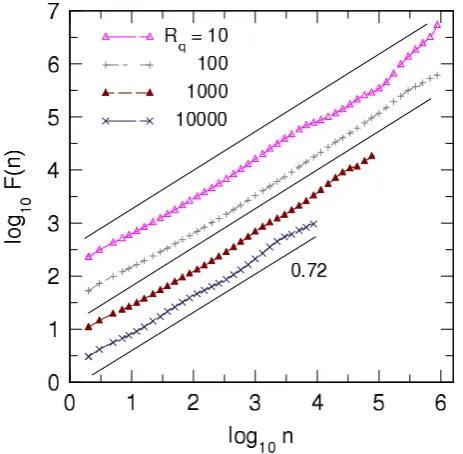
Fig. 6. DFA fluctuation functions for the sequence of return times obtained with a FD (γ = 0.01) and different thresholds corre-sponding to the mean return timesRqas indicated. nenumerates the return time sequence. The solid lines show the LTM exponent α= 0.72.

Fig. 5. (a) Simulated data (FD withγ=0.01) and (b) frequency distribution.

0 20000 40000 60000 80000

−6 −4 −2 0 2 4

6 a) Simulated data

Density

0.00 0.05 0.10 0.15 0.20 0.25 0.30

−5 0 5

b)

Fig. 5. (a) Simulated data (FD withγ = 0.01) and (b) frequency distribution.

Fig. 6. DFA fluctuation functions for the sequence of return times obtained with a FD (γ = 0.01) and different thresholds corre-sponding to the mean return timesRqas indicated. nenumerates the return time sequence. The solid lines show the LTM exponent

α= 0.72.

Fig. 6. DFA fluctuation functions for the sequence of return times

obtained with a FD (γ=0.01) and different thresholds correspond-ing to the mean return timesRq as indicated. nenumerates the return time sequence. The solid lines show the LTM exponent

α=0.72.

4.1 Return time distributions

The distributionpq(tr)for the return timestr is determined

for a thresholdqrelated to a mean return timeRq=100. The

analysis is analogous to Sect. 3.2. The distribution (Fig. 4c) is well approximated by a Weibull distribution. The 95% confidence interval (gray shaded) is determined by creat-ing 1000 time series with the same parameters. The shape and scale parameters areγ=0.2 and τ=0.29, respectively. The validity of the power law fit,pq∼tr−s with the exponent s=1.53, is restricted to tr≈10. . .500. The deviation from s=1.5, which is the 1/f limit of the stretched exponential, might originate in either:

Table 1. Values of: estimated parameters for Weibull and

power-law distributions (with 95% confidence intervals), and cutoffs for the Weibull (power-law) distribution.

temperature mixing ratio simulated data

shapeγ 0.21 (0.17, 0.27) 0.15 (0.11, 1.88) 0.19 (0.15, 0.25) scaleτ 0.36 (0.04, 1.94) 0.003 (10−5, 0.04) 0.29 (0.01, 2.68) exponents 1.74 (1.66, 1.85) 1.80 (1.69, 1.94) 1.53 (1.49, 1.57) cutoffk_min 4 (8) 5 (46) 5 (10)

(i) The conjecture that the stretched exponential exponent (see Eq. 8) is identical to the correlation exponentγ is not valid.

(ii) The streched exponential is not valid for very small

γ=0.01, i.e. near 1/f.

4.2 Potential predictability of extreme event return times For time series with weak LTM (correlation exponents

γ=0.4,0.7, Bunde et al., 2004) the sequencestr(n)

com-posed of extreme event return times show long-term correla-tions with similar LTM as the time series itself. To analyse this behavior in the vicinity of 1/f noise, the correlation ex-ponent is γ=0.01 (as in Sect. 4.1) and the extreme events are based on different thresholds providing the mean return timesRq=10,100,1000,10000. The total length of the time

series isN=108. Note that this is two decades longer than

N=221≈2.1·106in Eichner et al. (2007). The sequence of the return times is analyzed by detrended fluctuation anal-ysis (DFA). Figure 6 shows that the long-term correlation of the return times is described by a power-law fluctuation functionF (n)∼nα withα≈0.72 independent of the thresh-old and the mean return time; the indexn enumerates the return times. This corresponds to the power spectrum expo-nentβ≈0.44 (usingβ=2α−1) and the correlation exponent

(8)

564 R. Blender et al.: Extreme event return times 5 Conclusions

This paper presents an analysis of the extreme event re-turn time statistics for observed and simulated data with 1/f power spectra. The observed data is given by mea-surements of temperature and mixing ratio during TOGA-COARE (November 1992–February 1993) at the research vessel Kexue. In the time series of one minute resolution, 61 days with low numbers of missing values are extracted. Both time series show a scaling power spectrum,S(f )∼f−β, with

β=1. . .1.2; the correlation exponent inC(t )∼t−γ is related byγ=1−β. This result is determined by detrended fluctua-tion analysis and substantiated by a fit of a FARIMA (p, d,0) fractionally differenced autoregressive process which yields

d≈0.5 for the long-term behavior (β=2d). Hence, both time series are considered as 1/fnoise.

Extreme events are determined by Peak-Over-Threshold (POT) crossing. The observed return time distributions

pq(tr)are compared to a stretched exponential,∼exp(−tγ),

and a Weibull distribution,∼tγ−1exp(−tγ). According to the approach by Altmann and Kantz (2005) and Eichner et al. (2007), the stretched exponential distribution converges to a power-lawpq(tr)∼tr−s withs=1.5 forγ→0.

The return time distributions for the two observed time se-ries are better approximated by a Weibull distribution than by a power-law. If a power-law is fitted in the intermediate range of return times, the temperature yields a power-law ex-ponents=1.74, while the mixing ratio yieldss=1.8; both are distinctly different from the stretched exponential limit.

Simulated data is generated by a fractionally differenced autoregressive process with a power spectrum in the vicin-ity of the stationarvicin-ity threshold,β=0.99 (γ=0.01). As for the observational data, the Weibull distribution yields a con-vincing representation of the return time distributions, while a power-law can be excluded.

The simulated data is used to evaluate the potential pre-dictability of the extreme event return times. The LTM in the sequence of return times is analyzed by the detrended fluctuation analysis and reveals a power law fluctuation func-tionF (n)∼nα withα≈0.72 (correlation exponentγ¯≈0.56). Thus, the return time sequences show weaker long-term cor-relations than the original time series. This values is indepen-dent of the threshold and the mean return time. A possible reason is that short term random effects lead to level cross-ings which, thereby, perturb the overall LTM of the original time series.

The analysis leads to the following main conclusions for the behavior of extreme event return times in the 1/f limit:

(i) The return time distributions for time series in the vicin-ity of a 1/f power spectum are well approximated by the standard Weibull distribution. This is suggested by the observed time series and substantiated by the sim-ulated data. The stretched exponential (which differs

from Weibull by the absence of a prefactor) is likely to be convenient for weak LTM.

(ii) The sequence of return times shows LTM with

F (n)∼nα with α≈0.72 which is weaker than in the original time series (α=0.995). However, the correla-tionC(n)∼n−0.56is still promising for the prediction of return times.

Future analyses should consider the Weibull distribution as an alternative to the stretched exponential return time distri-bution for a wide range of LTM correlation coefficientsγ.

Acknowledgements. We like to thank the reviewers and the editor

for their useful comments. This work has been supported by the EC project E2C2, Contract No. 012975.

Edited by: B. D. Malamud

Reviewed by: H. Rust and three other anonymous referees

References

Abaimov, S. G., Turcotte, D. L., Shcherbakov, R., and Rundle, J. B.,: Recurrence and interoccurrence behavior of self-organized complex phenomena, Nonlin. Processes Geophys., 14, 455–464, 2007,

http://www.nonlin-processes-geophys.net/14/455/2007/. Altmann, E. G. and Kantz, H.: Recurrence time analysis, long-term

correlations, and extreme events, Phys. Rev. E, 71, 056106, 2005. Beran, J.: Statistics for long-memory processes, Chapman &

Hall/CRC Press, London, 315 pp., 1994.

Blender, R. and Fraedrich, K.: Long time memory in global warm-ing simulations, Geophys. Res. Lett., 30(14), 1769–1772, 2003. Bunde, A., Eichner, J. F., Havlin, S., and Kantelhardt, J. W.: Return

intervals of rare events in records with long-term persistence, Physica A, 342, 308–314, 2004.

Bunde, A., Eichner, J. F., Kantelhardt, J. W., and Havlin, S.: Long-term memory: A natural mechanism for the clustering of extreme events and anomalous residual times in climate records, Phys. Rev. Lett., 94, 048701, 2005.

Clauset, A., Shalizi, C. R., and Newman, M. E. J.: Power-law distri-butions in empirical data, http://arxiv.org/abs/0706.1062, 2007. Corral, A.: Long-term clustering, scaling, and universality in

the temporal occurrence of earthquakes, Phys. Rev. Lett., 92, 108501, 2004.

Eichner, J. F., Kantelhardt, J. W., Bunde, A., and Havlin, S.: Statis-tics of return intervals in long-term correlated records, Phys. Rev. E, 75, 011128, 2007.

Fraedrich, K. and Blender, R.: Scaling of atmosphere and ocean temperature correlations in observations and climate models, Phys. Rev. Lett., 90, 108501, 2003.

Hosking, J. R. M.: Fractional differencing, Biometrika, 68, 165– 176, 1981.

Huybers, P. and Curry, W.: Links between annual, Milankovitch and continuum temperature variability, Nature, 441, 329–332, 2006. Lucas, C. and Zipser, E. J.: Environmental variability during TOGA

COARE, J. Atmos. Sci., 57, 2333–2350, 2000.

(9)

Monetti, R. A., Havlin, S., and Bunde, A.: Long-term persistence in the sea surface temperature fluctuations, Physica A, 320, 581– 589, 2003.

Maraun, D., Rust, H. W., and Timmer, J.: Tempting long-term memory – on the interpretation of DFA results, Nonlin. Processes Geophys., 11, 495–503, 2004,

http://www.nonlin-processes-geophys.net/11/495/2004/. Newell, G. F. and Rosenblatt, M.: Zero crossing probabilities for

Gaussian stationary processes, Ann. Math. Stat. 33, 1306, 1962. Olla, P.: Return times for stochastic processes with power-law

scal-ing. Phys. Rev. E, 76, 011122, 2007.

Peng, C.-K., Buldyrev, S. V., Havlin, S., Simons, M., Stanley, H. E., and Goldberger, A. L.: On the mosaic organization of DNA sequences. Phys. Rev. E, 49, 1685–1689, 1994.

R Development Core Team, R: A language and environment for sta-tistical computing, Vienna, Austria, http://www.R-project.org, 2005.

Sornette, D.: Critical phenomena in natural sciences, 2nd ed., Springer Series in Synergetics, Springer-Verlag, Heidelberg, 528 p., 2006.

Webster, P. and Lukas, R.: TOGA COARE: the Coupled Ocean-Atmosphere Response Experiment, Bull. Amer. Meteor. Soc., 73, 1377–1416, 1992.

Weissman, M. B.: 1/f noise and other slow, nonexponential kinet-ics in condensed matter, Rev. Mod. Phys., 60, 537–571, 1988. Yano, J.-I., Fraedrich, K., and Blender, R.: Tropical convective

vari-ability as 1/f-noise, Journal of Climate, 14, 3608–3616, 2001. Yano, J.-I., Blender, R., Zhang, C., and Fraedrich, K.: 1/f-Noise and

pulse-like events in the tropical atmospheric surface variabilities: Convective self-criticality and impacts on ENSO, Quart. J. Roy. Meteorol. Soc., 130, 1697–1721, 2004.