www.atmos-meas-tech.net/9/3641/2016/ doi:10.5194/amt-9-3641-2016
© Author(s) 2016. CC Attribution 3.0 License.
Toward autonomous surface-based infrared remote sensing of polar
clouds: cloud-height retrievals
Penny M. Rowe1,2, Christopher J. Cox3,4, and Von P. Walden5 1NorthWest Research Associates, Redmond, WA, USA
2Physics Department, Universidad de Santiago de Chile, Santiago, Chile
3Cooperative Institute for Research in Environmental Sciences, University of Colorado, Boulder, CO, USA 4NOAA Earth System Research Laboratory, Physical Sciences Division, Boulder, CO, USA
5Department of Civil and Environmental Engineering, Washington State University, Pullman, WA, USA Correspondence to:Penny M. Rowe ([email protected])
Received: 12 February 2016 – Published in Atmos. Meas. Tech. Discuss.: 7 March 2016 Revised: 31 May 2016 – Accepted: 22 June 2016 – Published: 9 August 2016
Abstract. Polar regions are characterized by their remote-ness, making measurements challenging, but an improved knowledge of clouds and radiation is necessary to under-stand polar climate change. Infrared radiance spectrometers can operate continuously from the surface and have low power requirements relative to active sensors. Here we ex-plore the feasibility of retrieving cloud height with an in-frared spectrometer that would be designed for use in remote polar locations. Using a wide variety of simulated spectra of mixed-phase polar clouds at varying instrument resolutions, retrieval accuracy is explored using the CO2slicing/sorting and the minimum local emissivity variance (MLEV) meth-ods. In the absence of imposed errors and for clouds with op-tical depths greater than ∼0.3, cloud-height retrievals from simulated spectra using CO2slicing/sorting and MLEV are found to have roughly equivalent high accuracies: at an in-strument resolution of 0.5 cm−1, mean biases are found to be∼0.2 km for clouds with bases below 2 and−0.2 km for higher clouds. Accuracy is found to decrease with coarsen-ing resolution and become worse overall for MLEV than for CO2 slicing/sorting; however, the two methods have differ-ing sensitivity to different sources of error, suggestdiffer-ing an ap-proach that combines them. For expected errors in the at-mospheric state as well as both instrument noise and bias of 0.2 mW/(m2sr cm−1), at a resolution of 4 cm−1, average re-trieval errors are found to be less than ∼0.5 km for cloud bases within 1 km of the surface, increasing to ∼1.5 km at 4 km. This sensitivity indicates that a portable, surface-based infrared radiance spectrometer could provide an important
complement in remote locations to satellite-based measure-ments, for which retrievals of low-level cloud are challeng-ing.
1 Introduction
Measurements of cloud properties are needed to improve cli-mate and forecast models of the Arctic and Antarctic atmo-spheres (Hines et al., 2004; Town et al., 2007; Wesslen et al., 2014). Clouds have a strong impact on the polar regions, and recent work indicates that sensitivity to clouds may increase as polar regions warm (Cox et al., 2015b). At the same time, large errors have been found in atmospheric radiative fluxes and cloud radiative forcing in reanalysis products and cli-mate models, which have been partially attributed to errors in cloud-base heights (Walsh et al., 2009); for ERA-Interim, Wesslen et al. (2014) find that cloud-base height is often too high.
thus directly tied to, their radiative effect. However, passive satellite-based instruments are best suited for viewing the tops of clouds and have less sensitivity to the important re-gion of the atmosphere that affects the surface energy bud-get, that is, between the surface and the base of the cloud. Thus, satellite-based measurements should be complemented by surface-based measurements.
Atmospheric observatories that are capable of surface-based remote sensing of cloud properties exist in the Arc-tic at a small number of coastal and interior land stations; in addition, a number of field campaigns have been con-ducted over the Arctic Ocean (see Uttal et al., 2015, and ref-erences therein). In the Antarctic, field stations are sparsely located, principally on the coast, and have fewer instruments for measuring cloud properties than in the Arctic. In ad-dition to cloud measurements from existing field stations and past campaigns (Bromwich et al., 2012, and references therein), the Atmospheric Radiation Measurement (ARM) West Antarctic Radiation Experiment (AWARE) is making a broad suite of measurements from November 2015 to 2017. Nevertheless, there remains a dearth of surface-based remote sensors in the Antarctic. The lack of instrumentation at both poles is due largely to the expense and logistical challenge of deploying instruments in these remote regions. A lack of autonomous sensors prevents collection of data at loca-tions other than established staloca-tions. New instruments are needed that address these challenges, in particular designs intended for the purposes of both climate monitoring and process studies representing a more comprehensive range of regional high-latitude climates.
Surface-based infrared spectrometers, such as the At-mospheric Emitted Radiance Interferometer (AERI) of the ARM program, are proven instruments that have been used to retrieve cloud temperature or height in the Antarctic (Mahesh et al., 2001) and Arctic (Rathke et al., 2002). There have been a limited number of cloud-height retrievals from surface-based infrared spectrometers because cloud height is more typically measured by co-located active instruments. How-ever, a legacy of cloud-height retrievals from stand-alone passive infrared remote sensors on satellites has demon-strated the usefulness of this approach and led to refined re-trieval methodologies (e.g., Smith and Platt, 1978; Minnis et al., 2001; Kahn et al., 2007). Infrared spectrometer tech-nology can be relatively low-cost, with energy requirements that are considerably lower than active instrumentation such as lidar (e.g., Christensen et al., 2004). Thus, portable, au-tonomous infrared spectrometers are a viable solution for ac-quiring long-term, high temporal resolution, surface-based measurements of clouds and the atmospheric state from a more spatially diverse and comprehensive sample of the high latitudes, including over sea ice. Evaluating the requirements for accurate cloud-height retrievals is a first step towards de-velopment of such a system.
Here we evaluate the potential for using an autonomous infrared spectrometer capable of being deployed in remote
regions for retrieving cloud-base height. In particular, noise characteristics depend on instrument resolution (which lim-its the instrument throughput), and hence noise decreases as resolution becomes coarser. Thus we also test the effects of instrument resolution on the accuracy of cloud-height re-trievals. Since such an instrument is currently hypothetical, our analysis makes use of a simulated dataset from Cox et al. (2016). Using simulated data also affords a number of use-ful advantages for evaluating design aspects of an infrared spectrometer by permitting control over the sources of er-ror and maintaining a fixed and known standard for com-parison. This allows uncertainties associated with retrieval methodology and instrument characteristics to be isolated. Two established methods for retrieving cloud height using spectrally resolved infrared instruments, the minimum local emissivity variance (MLEV) technique (Huang et al., 2004) and the CO2slicing (e.g., Menzel et al., 1983; Mahesh et al., 2001) and sorting (Holz et al., 2006) technique, are further developed and intercompared here. Although these have been compared for satellite-based retrievals from upwelling radi-ances (Holz et al., 2006), they have not been compared for retrievals from downwelling radiances or with consideration of variability in noise characteristics and spectral sampling between different types of spectrometers, which are key engi-neering barriers to developing an autonomous surface-based system. Here we evaluate and compare these techniques to determine relative accuracies for surface-based retrievals of downwelling radiance in the Arctic and to constrain the in-strument requirements for providing cloud-height informa-tion from an infrared spectrometer that is designed for au-tonomous deployment.
2 Simulated radiances
ad-0 1 2 3 4 5 6 7 8 0
5 10 15 20 25
Height [km]
Frequency
of
occurrence
[%
]
(a) Base
Top
0 0.25 0.5 0.75 1 1.25 1.5 1.75 2 0
5 10 15 20 25
Thickness [km]
Frequency
of
occurrence
[%]
(b)
210 220 230 240 250 260 270 280 290 0
10 20 30
Temperature [K]
Frequency
of
occurrence
[N]
(c) Ice
Mix. Liq. All
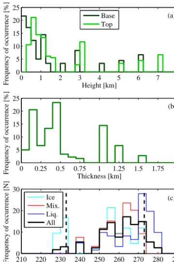
Figure 1. Reproduced from Cox et al. (2016). Distributions of
macrophysical properties for 222 simulated clouds.(a)Cloud-base height (black) and cloud-top height (green);(b)physical thickness; (c)cloud mean temperature. The vertical lines in(c)represent the physical limits imposed on the cloud phase; liquid is present above the lower limit, while ice is present below the upper limit.
ditional spectra created in a similar manner). These are de-scribed below.
2.1 Base dataset
For the base dataset, a variety of typical Arctic atmospheres are represented, including conditions for all four seasons and a variety of cloud types. Because of the high incidence of mixed-phase clouds in polar regions, both single-phase and mixed-phase clouds are included. Temperature-dependent single-scattering parameters are used for liquid (see Rowe et al., 2013, and references therein), while single scatter-ing parameters for ice spheres are from Warren and Brandt (2008). In the base dataset, mixed-phase clouds are mod-eled as externally mixed in a single layer. Cloud-base heights range from 0 to 7 km with temperatures ranging from 225 to 283 K. Figure 1, reproduced from Cox et al. (2016), shows the distributions of cloud height, thickness, and temperature for the base dataset. Overall, the atmospheric temperature and humidity profiles as well as the cloud optical depths, phases, effective radii, and cloud heights used in the model are intended to be realistic for the Arctic. Temperature inver-sions are included and cloud heights are typically low with fewer high clouds. Total cloud optical depth referenced to
the visible region (hereafter termed cloud optical depth for brevity) varies from 0 to 12. Cloud optical depth divided by cloud physical thickness (a proxy for visible extinction co-efficient) varies from 0 to 0.01 m−1 near the surface and 0 to 0.001 m−1 above 4 km. To test the limits of cloud prop-erty retrievals, a few extreme and/or less likely cases were included. For example, the dataset includes a few cases of clouds with optical depths that are extremely low (<0.2) and includes high clouds that are optically thick as well as thin. Precipitable water vapor (PWV) amounts span the range typ-ical of the polar regions, but some cases are included that are quite high for the polar regions (mean=1 cm, standard deviation=0.72 cm, maximum=3 cm, minimum=0.2 cm). The base set is comprised of 222 clouds. Of these, 157 have bases below 2 km (hereafter referred to as “low clouds”) and 65 have bases above 2 km (hereafter referred to as “high clouds”). While all simulations are for single-layer clouds, the cloud layer spans multiple model layers for 69 % of the low clouds (108 out of 157). This base set allows determi-nation of the accuracy of the retrievals for varying atmo-spheric temperature and humidity profiles, precipitable water vapor amounts, cloud heights, temperatures, optical depths, ice fractions, and effective radii for clouds that are otherwise simplistic. In this work, the base dataset is used for analyses unless otherwise noted.
Unlike clouds in the base dataset, real clouds are verti-cally and horizontally inhomogeneous, vary temporally, and consist of a variety of ice habits. Simulations that account for these variations were created with other atmospheric and cloud properties held constant. For this purpose, subsets of the base set of clouds were selected.
2.2 Subset: cloud inhomogeneity
Cloud inhomogeneity includes vertical variation through the cloud, horizontal variation over the instrument field of view, and variation with time during the timespan of a measure-ment. For testing the effects of cloud inhomogeneity, cases were selected in which clouds span multiple model layers (to simulate vertically varying cloud properties), have opti-cal depths greater than 0.5 (retrievals using the base dataset indicate that for optical depths less than about 0.5 the cloud signal is often too low for accurate retrievals), and are mixed phase (ice fractions between 0.2 and 0.8). This subset con-sists of 23 cases. From this subset, simulations were rerun with various attributes modified. To allow isolation of errors due to various assumptions, each new simulation was mod-ified in only one respect; in all 92 additional spectra were created. Modifications include the following.
each model layer. Thus, for a three-model-layer cloud with layers of equal physical thickness, the top-layer optical depth would be 25 % of the total, the middle layer 50 %, and the bottom layer 25 %. The total optical depth through the cloud is the same as in the corresponding base dataset case, and ice fraction (with respect to optical depth) is kept the same.
For horizontally and temporally varying cloud simula-tions, the cloud measurement is expected to be a linear com-bination of spectra of different clouds. Such spectra were cre-ated by averaging spectra. First, an additional set of simula-tions for physically thin clouds was created by placing all cloud optical depth in the middle model layer. Simulations of these physically thin clouds, the set of vertically inhomo-geneous clouds described above, and the base dataset were then averaged to simulate time averages of clouds that vary from physically thin and dense to thicker and more diffuse.
Because measurements indicate that Arctic clouds are of-ten composed of an ice layer topped by a liquid layer, liquid-topped clouds were created by placing all cloud liquid in the top model layer and placing all ice in the model layers below. Total optical depths of liquid and ice were kept the same as in the corresponding cases from the base dataset.
2.3 Subset: ice habit
To create a subset of cases suitable for testing the effect of ice habit on retrievals, cases were selected for which ice op-tical depth was greater than 0.5 and ice fraction was greater than 0.5 %. While 79 such cases exist, 15 representative cases were selected. These include seven low clouds and eight high clouds. For both low and high clouds, winter, summer, and transition (spring/fall) seasons are represented, and optical depth varies from 0.8 to 5. The 15 cases, for five ice habits, represent 75 additional simulations. Spectra were simulated for this subset for the following ice habits: hollow bullet rosettes, smooth plates, rough plates, smooth solid columns, and rough solid columns, using the single scattering param-eters of Yang et al. (2005, 2013). Further details about these simulations are provided in Cox et al. (2016).
2.4 Spectral resolution
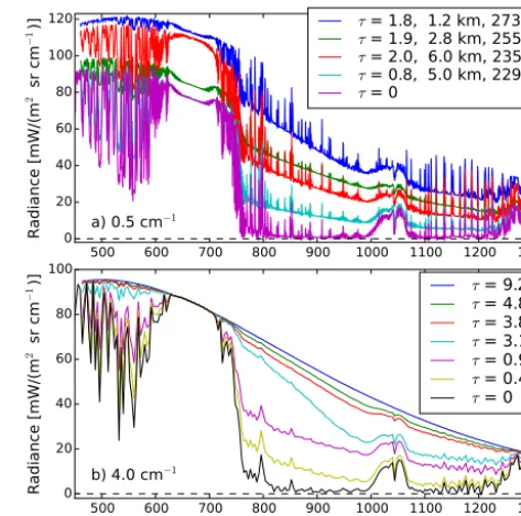
The perfect resolution spectra were convolved with sinc functions to create sets of simulated cloudy-sky radiances at resolutions of 0.1, 0.5, 1, 2, 4, and 8 cm−1. These simu-lated cloudy-sky radiances serve as the “observations”,Robs, used to test the cloud-height retrievals. Some examples are shown in Fig. 2 at resolutions of 0.5 and 4 cm−1. Absorp-tion lines are clearly evident at the finer spectral resoluAbsorp-tion but are smoothed out at the coarser resolution. At around 667 cm−1 the radiance depends on the surface tempera-ture and clouds have negligible effect. Moving from 667 to 710 cm−1, the effects of temperature inversions are evident: a decreasing radiance indicates temperatures decreasing with height, whereas an increasing radiance indicates
tempera-W
Figure 2. (a) Downwelling radiance spectra at a resolution of
0.5 cm−1, for visible optical depths, cloud-base heights, and tem-peratures shown in legend.(b)Same but at a resolution of 4 cm−1 for a cloud-base height of 1.4 km and temperature of 249 K.
tures increasing with height. In panel (a), the uppermost three spectra have similar optical depths (≈2) but different cloud-base temperatures; the radiance decreases in the window re-gion (750 to 1300 cm−1) with decreasing cloud temperature. (Note that the lower two spectra have lower optical depths, with an optical depth of 0 indicating clear skies.) In panel (b), atmospheric profiles are identical and the cloud-base height is 1.4 km for all clouds, but the optical depth varies. The radi-ance decreases with decreasing optical depth in the window region. Note also that the shapes of the spectra differ for op-tical depths of 3.8 and 3.1; spectral shape also depends on thermodynamic phase, effective radius, and ice habit.
3 Cloud-height retrieval methods
atmo-spheric transmittance. Finally, we describe modifications to the MLEV and CO2 slicing/sorting methods made in this work. For MLEV, the method is modified for downwelling radiances, while for CO2slicing and sorting the best aspects of the methods of Holz et al. (2006) and Mahesh et al. (2001) are combined, based on experimentation with retrievals from the dataset of simulated Arctic downwelling radiances. The retrievals all assume a zenith view.
3.1 Cloud emissivity
Both MLEV and CO2slicing depend on approximations in-volving the cloud emissivity over the wavenumber range of interest: MLEV assumes it is smoothly varying with wavenumber, while CO2 slicing traditionally assumes it is constant. Ignoring scattering, the observed downwelling ra-diance for a zenith view,Robs, is
Robs≈ TOA Z
0
B(T (z))dt
dzdz, (1)
where the parentheses represent functionality,Bis the Planck function,T is temperature,zis height,tis the transmittance from the surface toz, and the integration is from the surface (height of 0) to the top of atmosphere (TOA). The integral can be broken up into contributions from the surface to the cloud base (base), from cloud base to cloud top (top), and from cloud top to the TOA. The radiance contribution from the surface to the cloud base (Rc) is unaffected by the pres-ence of the cloud.
Robs≈Rc+ top Z
base
B(T (z))dt dzdz+
TOA Z
top
B(T (z))dt
dzdz (2)
If we assume that the cloud is in an infinitesimally thin layer (zbase=ztop) devoid of gases (i.e., gaseous transmit-tance within the cloud equals unity), a number of simplifi-cations are possible. We letB(T (zbase))=B(T (ztop))=Bc, the Planck function at the cloud temperature. The first in-tegral on the right-hand side can then be solved to give Bc[1−tcld]tc, wheretcis the gaseous transmittance from the surface to the cloud base andtcldis the cloud transmittance. We have
Robs≈Rc+Bctc[1−tcld] +tcld TOA Z
top
B(T (z))dt
0
dzdz, (3)
wheret0 is the cloud-free transmittance from the surface to heightz. The final integral is the radiance contribution from above the cloud that makes it through the gaseous atmo-sphere below the cloud; it is independent of the cloud pres-ence and is equal to Rclr−Rc. Assuming local thermody-namic equilibrium (and again ignoring scattering), the cloud
absorptivity equals the emissivity, so that(1−tcld)=. We can ignore the cloud fraction when the instrument field of view is small, but the emissivity can also be thought of as an effective emissivity that takes into account any patchiness in the cloud within the field of view.
Robs≈Rc+Bctc+ [Rclr−Rc]tcld (4) Substituting in (1−) fortcldand simplifying gives
Robs≈Rclr+[Bctc+Rc−Rclr]. (5) The equation can be rearranged to solve for the emissivity: ≈ Robs−Rclr
Bctc+Rc−Rclr
. (6)
Eq. (6) is comparable to Eq. (4) of Huang et al. (2004) and Eq. (2) of Holz et al. (2006), whereRcld=Bctc+Rc. The equation in the form shown here demonstrates that cloud height and effective emissivity are very closely connected, making cloud-height retrievals challenging.Bc depends on cloud temperature, which in turn depends on cloud height, andtc andRc both depend on cloud height. Thus errors in cloud height can be largely accounted for by errors in emis-sivity.
The right-hand side of Eq. (6) depends on the observed ra-diance,Robs, and quantities that can be calculated based on knowledge of the cloud-free atmospheric state. In this work, RclrandRcare calculated from atmospheric profiles of pres-sure, temperature, and trace gas amounts, using similar ra-diative transfer calculations as those performed by LBLRTM (Clough et al., 1992). Rclr need only be calculated once, whereas tc and Rc are calculated for each potential cloud height.Rclr,tc, andRcall include gaseous contributions and therefore vary rapidly with frequency. By contrast,andBc should vary slowly with frequency.
To summarize the model assumptions, they include mod-eling the atmosphere as a plane-parallel, layered atmosphere in local thermodynamic equilibrium, ignoring scattering, as-suming the cloud is in an infinitesimally thin layer devoid of gases, and assuming that the emissivity is slowly varying or constant with frequency over∼710–950 cm−1.
3.2 MLEV
To find the MLEV,is calculated for each potential cloud height,c, for wavenumbers between limits ν1 andν2. The “local” emissivity variance (LEV) is then calculated accord-ing to Eq. (5) of Huang et al. (2004):
LEVc=
ν2
X
ν1
(c,ν− hc,νi)2, (7)
ν2but rather over a small wavenumber region (1ν) aboutν:
h(c, ν)i = 1 1ν
ν+1ν/2 X
ν−1ν/2
c,ν. (8)
Huang et al. (2004) use ν1=750 and ν2=950 cm−1 in Eq. (7) and use an interval of1ν=5 cm−1in Eq. (8). When Eq. (7) is calculated with an incorrect height, errors in the calculated values oftcandRcresult in errors in the calculated effective emissivity that vary rapidly with frequency due to the dependence oftcandRcon trace gases, causing the LEV to be large. Thus the correct cloud height is retrieved as that corresponding to the minimum LEV, or MLEV.
In this work, the MLEV method is performed similarly to that of Huang et al. (2004) but for downwelling radiances and for a variety of different spectral resolutions. Furthermore, all values are calculated for the desired instrument resolution. This is done by convolvingRclr,tc, andRcwith a sinc func-tion with the desired linewidth. As in Huang et al. (2004), we useν1=750 andν2=950 cm−1. For resolutions of 0.5 and 1 cm−1, we use an interval of1ν=5 cm−1in Eq. (8) (cor-responding to averaging over 10 or 5 spectral points, respec-tively), like Huang et al. (2004). However, for a resolution of 2 cm−1, we use1ν=10 cm−1(average over 5 points), and for resolutions of 4 and 8 cm−1we use1ν=24 cm−1 (aver-age over 6 or 3 points, respectively). Small variations about these values were found to give similar results.
The steps for MLEV are as follows.
1. Choose model heights (layer boundaries) for the model atmosphere. CalculateRclr. CalculateRc,Bc, andtcfor each model height for the clear-sky atmosphere based on best estimates of temperature, water vapor, and trace gas amounts.
2. Calculate the LEV (Eqs. 6–8) for each trial cloud height. 3. Find the height that corresponds to the MLEV.
3.3 CO2slicing and sorting
In Mahesh et al. (2001), CO2slicing makes use of the varia-tion in the absorpvaria-tion coefficient of the CO2band from∼700 to 755 cm−1, where CO2emission dominates. (Unlike H2O, CO2is a well-mixed gas and thus can be estimated fairly ac-curately from surface measurements.) Rearranging Eq. (5), including the wavenumber dependence explicitly, and divid-ing both sides by the same quantities at a reference wavenum-ber,ν0, gives
Robs(ν)−Rclr(ν) Robs(ν0)−Rclr(ν0)
= (9)
(ν)[Bc(ν)tc(ν)+Rc(ν)−Rclr(ν)] (ν0)[Bc(ν0)tc(ν0)+Rc(ν0)−Rclr(ν0)]
.
The value of νis varied from∼700 to 755 cm−1, whileν0 is chosen to be a wavenumber close to this spectral region
but where the absorption coefficient of CO2is small enough (i.e., the transmittance is large enough) that the downwelling radiance is sensitive to the entire atmospheric column (Ma-hesh et al., 2001, chose∼812 cm−1). It is next assumed that the emissivity is constant from 700 to 812 cm−1, so that the emissivity terms cancel.
Robs(ν)−Rclr(ν) Robs(ν0)−Rclr(ν0)
= (10)
Bc(ν)tc(ν)+Rc(ν)−Rclr(ν) Bc(ν0)tc(ν0)+Rc(ν0)−Rclr(ν0)
The left-hand side (LHS) of Eq. (10) is constant, while the right-hand side (RHS) varies with assumed cloud height. So-lutions are found at each wavenumber where the RHS equals the LHS, giving a retrieved cloud height for eachν. When the RHS is not equal to the LHS at any height, the solution is found where the magnitude of the difference (RHS−LHS) is smallest. Due to model and measurement errors, retrieved cloud heights vary for different values ofν. (Note that Ma-hesh et al., 2001, retrieve cloud-base pressure rather than height; in this work, cloud-base height is retrieved.) Mahesh et al. take a weighted average of the results obtained, where the weights are the change in the RHS with a change in the pressure at the cloud base, determined in a 10 hPa interval centered about the retrieved cloud-base pressure. This typi-cally provides more weight to wavenumbers with “e-folding” distances close to the cloud base.
Multiple solutions may exist at a givenνdue to errors or due to the presence of near-surface temperature inversions, which are common in the polar regions. Due to a tempera-ture inversion, the cloud temperatempera-ture may exist at more than one height. Because the retrieval methodology relies to a large extent on sensitivity to cloud temperature (rather than height), choosing between heights having the same temper-ature can be challenging. To do this, the best result is de-termined for each set of solutions (e.g., the set below the inversion and the set above the inversion). Then, to choose between sets of cloud bases above and below a temperature inversion, Mahesh et al. (2001) perform a second step us-ing “short-sighted” wavenumbers. Short-sighted wavenum-bers are those with low transmittances, and are sensitive to low clouds but not high clouds. Mahesh et al. find the per-centage of short-sighted wavenumbers at which a cloud is detected. When this is large, the cloud base is assumed to be within the inversion; when it is small, the cloud base is assumed to be above the inversion.
Holz et al. (2006) use clear-sky brightness temperature as a proxy for clear-sky transmittance. (As will be discussed, this is a reasonable proxy when temperatures decrease with height in the troposphere, which is not always the case for this work.) First, clear-sky brightness temperatures are sorted. The sorted index is then applied to cloudy-sky ness temperatures. Sorted clear-sky and cloudy-sky bright-ness temperatures are then compared to determine at which wavenumbers they differ. Sorted wavenumbers are only used in the retrieval when the clear-sky and cloudy-sky brightness temperatures differ. This sets the lower limit in the gaseous transmittance such that wavenumbers that have little sensi-tivity to the cloud are excluded from the cloud-height de-termination. An upper limit in gaseous transmittance is also selected, based on where the slope of the brightness temper-ature decreases. Finally, Holz et al. found results were im-proved when only wavenumbers between strong CO2 absorp-tion lines were used.
Once the subset of wavenumbers to be used has been determined, a unique cloud height is determined for each wavenumber in a similar manner as for CO2slicing, but us-ing a different formulation, which is designed for upwellus-ing radiances (see Eq. 1 of Holz et al., 2006).
After a unique cloud height has been found for each wavenumber, the method for determining the best overall cloud height also differs from that of Mahesh et al. (2001). Instead of weighting the cloud heights, an error function is computed for each retrieved cloud height,c.
Err=X
ν0
Robs(ν)−Rclr(ν) (11) −c(ν0)[Bc(ν)tc(ν)+Rc(ν)−Rclr(ν)]
The sum is over the selected wavenumbers,ν0. The optimal cloud height is chosen as that which minimizes this equation. This work uses aspects of the CO2slicing method of Ma-hesh et al. (2001) as well as the CO2slicing/sorting method of Holz et al. (2006) and additional adaptations for compu-tational efficiency and for cloud retrievals specifically from downwelling radiance measurements made in the polar re-gions. Based on detailed sensitivity studies and trial and er-ror, the following modifications were made.
CO2 sorting is applied slightly differently in this work. The use of brightness temperature as a proxy for transmit-tance, as in Holz et al. (2006), is not a good approximation in the polar regions. While gaseous transmittance, which is de-fined relative to the surface, always decreases with height, clear-sky brightness temperatures do not always decrease with height in the polar regions; they can increase with height within near-surface temperature inversions, which are com-mon in the polar regions. Thus in our method, wavenumbers are sorted by gaseous transmittance from the surface to the TOA, tTOA. The gaseous transmittances are calculated for each measured radiance spectrum (at the desired resolution) based on the clear-sky atmospheric state and then sorted.
Another difference in our application of sorting involves setting the threshold for choosing the wavenumbers to use. Within the spectral range of 700 to 750 cm−1, at some wavenumbers CO2 transmits so little radiance that there is little sensitivity to cloud. At these wavenumbers,Robs−Rclr is expected to be on the order of the uncertainty. Thus a threshold is needed for which there is adequate cloud sig-nal for the retrieval. A threshold of 0.5 RU is used here (1 RU, or radiance unit, is defined to be 1 mW/(m2sr cm−1)). The gaseous transmittance tthresh determined as the trans-mittance for which the magnitude ofRobs−Rclris equal to 0.5 RU, and wavenumbers (ν) are selected that correspond to tTOA≥tthresh. A final difference is that an upper wavenum-ber cutoff of 755 cm−1is used, rather than estimating a cut-off based on the slope of the brightness temperature; the re-trieval is not sensitive to small variations in the choice of upper wavenumber.
Like Mahesh et al. (2001), we use short-sighted wavenum-bers to distinguish between multiple solutions. However, whereas Mahesh et al. found that wavenumbers between 670 and 700 cm−1 are sensitive to clouds within the inversion, this wavenumber range was found to have negligible sensi-tivity to clouds at any height for the atmospheric profiles used here. Instead, the best wavenumber range for the atmospheric profiles used here is found to be 705 to 715 cm−1. In addition, sensitivity studies indicate that a method that gives more ac-curate results than the method employed by Mahesh et al. is to once more find the solution that minimizes the error function given in Eq. (11), this time summing over the short-sighted wavenumbers (step 10 below). These short-short-sighted wavenumbers are where the transmittance is low and thus generally represent wavenumbers that were excluded in cal-culating the error function previously. The steps of the CO2 slicing/sorting method used in this work are summarized as follows.
1. Choose model heights (layer boundaries) for the model atmosphere. CalculateRclr. CalculateRc,Bc, andtcfor each model height for the clear-sky atmosphere based on best estimates of temperature, water vapor, and trace gas amounts.
2. Calculate the LHS of Eq. (10).
3. Calculate the RHS of Eq (10) for each model height and for each wavenumber.
4. Use CO2sorting to choose the best set of wavenumbers for the retrieval; these are typically between 720 and 755 cm−1.
5. Find the height(s) at which the LHS and RHS agree best (interpolate to find where they cross or, if they never cross, determine where the difference is a minimum) for each wavenumber selected by CO2sorting.
This yields sets of cloud heights retrieved, comprised of one height for each selected wavenumber within each set, with corresponding reference emissivities. For ex-ample, there might be a set of cloud heights retrieved (clower set(ν)) corresponding to heights below the inver-sion and a set (chigher set(ν)) above the inversion. 7. Calculate the error function as in Eq. (11) for the height
retrieved at the first wavenumber,c=clower set(ν=ν1), using the corresponding c(ν0) andBc(ν), tc(ν), and Rc(ν).
8. Repeat step 7 for each of the remaining selected wavenumbers (ν=ν2, etc). Findzc,lower set that corre-sponds to the minimum error. This yields a single cloud-height retrieval (cret, lower set).
9. Repeat 7 and 8 for the higher set of retrieved heights, yielding a single cloud-height retrieval (cret, higher set). 10. To choose betweencret, lower set andcret, higher set,
calcu-late the error function again for each of them. However, this time use the short-sighted wavenumbers; these are typically between 705 and 715 cm−1.
4 Results
In this section we demonstrate cloud-height retrieval accu-racy for the simulated spectra, including comparison of the results of the MLEV and CO2 slicing/sorting methods as adapted for this work against the true cloud-base heights, and characterize the effects of ice habit, cloud inhomogene-ity, temporal averaging of measured spectra, and sources of error. To understand how different hypothetical instrument specifications and varying amounts of ancillary information affect the results, the comparisons are made with and with-out imposed errors (e.g., instrument noise and bias and un-certainty in the water vapor and temperature profiles) and as functions of instrument resolution.
4.1 Cloud mask and retrieval capability
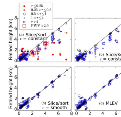
An important aspect of a cloud-height retrieval algorithm is that it must be able to determine whether there is a cloud present. Figure 3a shows a scatter plot of cloud height re-trieved using CO2slicing/sorting vs. true cloud-base height, for the base dataset. For these retrievals, no errors were im-posed, so the only error present is model error. The spectral resolution is 0.5 cm−1. The points are color-coded according to the cloud optical depth (in a real experiment, the optical depth will not be known). Cases with high PWV(>2.9 cm) are indicated in red boxes; these points will be discussed later. The true cloud bases are offset by a small random factor so that the points are spread out slightly for better visibility; the discrete cloud-base heights are evident for bases between 2 and 7 km.
Figure 3.Retrieved cloud height vs. true cloud base for cases with
no error and a simulated instrument resolution of 0.5 cm−1. The CO2slicing/sorting method (“Slice/Sort” in the figure) and MLEV methods are described in the text. In the figure, a small positive random number (mean of 0.2 km) was added to heights above 2 km to separate points for clarity.
Retrieved cloud-base heights for clouds with very low op-tical depths (less than 0.5; red and orange points) stand out as having larger retrieval errors. These points constitute clouds that are below the radiance detection threshold and therefore need to be removed from the analysis. The cloud mask is set according to a threshold for a difference between measured and simulated radiance; for the wavenumbers selected using CO2sorting, a requirement that the root mean square (RMS) difference between observed and clear-sky radiances differ by at least 2.2 RU is found to remove most low-accuracy points, as shown in Fig. 3b. All cases with cloud optical depths below 0.25 were removed and many of the clouds with optical depths below 0.5 were removed.
Robs(ν)−Rclr(ν) Robs(ν0)−Rclr(ν0)
= (12)
c,rat(ν)
Bc(ν)tc(ν)+Rc(ν)−Rclr(ν) Bc(ν0)tc(ν0)+Rc(ν0)−Rclr(ν0)
,
wherec,rat(ν)is determined at each trial cloud height (c) as an estimate of the ratio of the emissivity atνto the emissiv-ity atν0. For each trial heightc,rat(ν)is determined by first calculating the emissivity,c(ν), according to Eq. (6). While
c(ν)should be smooth, the observed value is highly variable
due to errors. Errors are expected to be lowest where the sig-nal is strongest. Thus the next step is to select the wavenum-bers where the signal is the strongest; for this a subset of the wavenumbers selected by CO2 sorting is used. When fewer than 16 wavenumbers are selected by CO2sorting, then no emissivity smoothing is attempted;c,rat(ν)is set to one; that is, Eq. (12) is abandoned in favor of Eq. (10). When at least 16 wavenumbers are selected by CO2 sorting, then the 16 to 30 points with the highest signal are used. A straight line is fitted to the emissivity at the selected wavenumbers, and its value is divided by c(ν0) to get an equation for c,rat for the selected wavenumbers. This equation is used for all wavenumbers within the range of the first and last of the se-lected wavenumbers. However, outside this range,c,ratis set to 1 because the weakness of the signal prohibits obtaining an estimate of the emissivity that is better than the assump-tion c(ν)=c(ν0), and examination of the true emissivity indicates that it may not continue to fall on the straight line determined by the fit at the selected wavenumbers.
Using a smooth, rather than constant, emissivity removes much of the low bias observed in Fig. 3b for clouds with bases above 2 km, as shown in Fig. 3c.
Returning to cases with high PWV (red boxes in panel a), note that these occur for cloud-base heights near 2 and 4 km. We see in panels (c) and (d) that these clouds are retrieved quite accurately. It is generally true that these higher-PWV cases can be retrieved accurately even when errors are im-posed, except for when large errors exist in PWV itself.
Figure 3d shows the scatter plot for cloud heights retrieved using MLEV. Comparing Fig. 3c and d, we see that both CO2 slicing/sorting and MLEV are quite accurate for single-layer clouds in the absence of imposed errors.
fig:resultsScatterErrspt5fig:resultsScatterErrs4
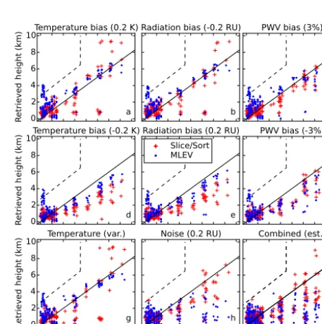
In a real experiment, there are errors in the observed ra-diance (noise or bias) and in knowledge of the atmospheric state, most notably temperature and humidity. To probe the effects of these sources of error, cloud heights are retrieved with errors imposed on the temperature or water vapor pro-files used in the retrieval or on the simulation of “observed” radiance (noise or radiation bias). Detailed studies of a va-riety of errors are summarized in Fig. 4 for a resolution of 0.5 cm−1and Fig. 5 for a resolution of 4.0 cm−1. The pan-els of these figures are scatter plots similar to Fig. 3c and d, but both CO2 slicing/sorting (blue pluses) and MLEV (red
c b c b c b
Figure 4.Retrieved vs. true cloud base for cases with the errors
shown in the titles for the CO2 slicing/sorting (Slice/Sort) and MLEV methods (at a resolution of 0.5 cm−1; see text for descrip-tion of errors). The dashed lines indicate the upper left region where points rarely lie.
b b
b c c
c
Figure 5.Retrieved vs. true cloud base for cases with the errors
Table 1.Errors in retrieved cloud height for clouds with bases below 2 km using the CO2slicing/sorting and MLEV retrieval methods at a resolution of 0.5 cm−1. Errors were determined by imposing a source of error (source) on either the cloudy-sky radiance – noise or radiation bias (bias) – or on the simulated radiances used in the retrieval. For profiles, biases were imposed at all heights, except for variable temperature errors (var.; see text) and errors in the tem-perature inversion (inv.; see text). The mean error (mean) and the standard deviation (SD) of the errors in retrieved cloud height are given. There were 157 cases, of which some were omitted based on screening (omit). The final two rows show estimates of the com-bined error for realistic sources of errors, calculated as described in the text.
CO2slicing/sorting MLEV
Source Value Mean SD Mean SD Omit
(km) (km) (km) (km) (no.)
None – 0.16 0.34 0.14 0.48 30
Noise 0.2 0.13 0.38 0.07 0.40 30
Bias (RU) 0.2 −0.02 0.34 0.03 0.48 29
Bias (RU) −0.2 0.27 0.37 0.27 0.38 33
Temp. (K) 0.2 0.30 0.35 0.21 0.48 33
Temp. (K) −0.2 −0.01 0.34 0.02 0.49 29
Temp. (K) var. 0.28 0.34 0.22 0.45 30
Temp. (K) inv. 0.39 1.00 0.14 0.62 30
PWV (%) 3 0.16 0.34 0.19 0.49 31
PWV (%) −3 0.14 0.35 0.05 0.61 29
PWV (%) 10 0.16 0.34 0.21 0.60 34
PWV (%) −10 0.13 0.36 −0.12 0.67 26
Combined – 0.23 0.38 0.18 0.49 34
Combined – 0.01 0.33 −0.05 0.45 27
dots) are plotted in each panel. Error sources and amounts are given in the titles (the black dashed line is discussed in Sect. 5.2), and mean errors and the standard deviations of errors are given in Tables 1 and 2. Errors are calculated as re-trieved cloud height minus true cloud base. Panels a–f show the results of biases in temperature, measured radiance, and PWV. Positive temperature biases cause biases in simulated radiances that are fairly smooth spectrally and thus have a very similar effect as negative radiation biases, and likewise for negative temperature biases and positive radiation biases. However, for water vapor, the effect is complicated by spec-trally varying line strengths, and PWV biases affect retrievals differently, particularly positive PWV biases. Random errors in temperature (see Tables 1 and 2) and PWV (not shown) were also tested but were found to have a smaller effect than bias errors due to partial cancellation. The effect of noise in measured radiation is shown in panel (h). Larger PWV bi-ases were also tested (10%; see Tables 1 and 2, not shown in figure). In addition, errors due to failing to capture the tem-perature inversion were calculated, as well as the effects of estimated temperature and PWV errors based on errors found in reanalysis data. Failing to capture temperature inversions can have a large effect on low clouds (Fig. 4g). Expected er-rors in reanalysis data cause retrieval erer-rors of similar mag-nitude as for biases in temperature (Fig. 5g) and PWV (not
Table 2. Errors in retrieved cloud height for clouds with bases
≥2 km using the CO2slicing/sorting and MLEV retrieval methods at a resolution of 0.5 cm−1. Errors were determined by imposing a source of error (source) on either the cloudy-sky radiance – noise or radiation bias (bias) – or on the simulated radiances used in the retrieval. For profiles, biases were imposed at all heights, except for variable temperature errors (var.) and errors in the temperature in-version (inv.; see text). The mean error (mean) and the standard de-viation (SD) of the errors in retrieved cloud height are given. There were 65 cases, of which some were omitted based on screening (omit). The final two rows show estimates of the combined error for realistic sources of errors, calculated as described in the text.
CO2slicing/sorting MLEV
Source Value Mean SD Mean SD Omit
(km) (km) (km) (km) (no.)
None – −0.10 0.33 0.01 0.19 32
Noise 0.2 −0.16 0.95 −1.28 1.27 32
Bias (RU) 0.2 −1.10 0.58 −0.69 0.35 29
Bias (RU) −0.2 0.60 1.63 0.38 0.20 32
Temp. (K) 0.2 0.87 1.80 0.44 0.24 32
Temp. (K) −0.2 −1.36 1.10 −0.86 0.46 29
Temp. (K) var. 1.02 1.74 −0.16 0.41 32
Temp. (K) inv. −0.58 1.23 −0.55 0.91 32
PWV (%) 3 0.11 0.47 0.01 0.70 33
PWV (%) −3 −0.30 0.50 −1.02 0.76 27
PWV (%) 10 0.54 0.87 −2.24 1.92 35
PWV (%) −10 −0.84 0.74 −2.74 1.66 22
Combined – 0.67 1.73 −1.28 1.60 33
Combined – −1.04 0.67 −1.99 1.28 27
Table 3.Errors in retrieved cloud height for macroscopically vary-ing clouds (see text), usvary-ing the CO2slicing/sorting and MLEV re-trieval methods at a resolution of 0.5 cm−1. For the upper set of cases (error=n), no errors were imposed on the retrieval, while for the lower set of cases (error=y) noise of 0.1 mW/(m2sr cm−1) and temperature bias of 0.1 K were imposed. The mean error (mean) and the standard deviation (SD) of the errors in retrieved cloud height are given.
CO2slicing/sorting MLEV
Cloud type Error Mean SD Mean SD
(km) (km) (km) (km)
Dense n 0.20 0.35 0.11 0.39
Diffuse n 0.25 0.33 0.35 0.55
Inhomogeneous n 0.36 0.42 0.43 0.57
Temporally varying n 0.24 0.27 0.23 0.41
Liquid topped n 0.25 0.34 0.35 0.56
Dense y 0.11 0.47 0.12 0.49
Diffuse y 0.15 0.37 0.21 0.50
Inhomogeneous y 0.21 0.36 0.31 0.44
Temporally varying y 0.19 0.45 0.19 0.49
Liquid topped y 0.23 0.57 0.24 0.49
in the presence of biases in the observed radiance and biases in temperature, while CO2slicing/sorting is more accurate in the presence of noise in the observed radiance and biases in water vapor.
Factors that complicate how errors affect retrievals using CO2slicing/sorting include errors in the fitting of the emis-sivity to a smooth function and changes in the strength of the apparent cloud signal, which can affect screening-out due to low signal. For example, positive biases can make the cloud signal look stronger (fewer cases screened out), while neg-ative biases can make it look weaker (more cases screened out). For MLEV, the consequences of errors are not as clear as for CO2slicing/sorting; indeed, both positive and negative biases in the water vapor profile (expressed as PWV in the figure) result in negative biases in retrieved cloud height. 4.3 Dependence of cloud-height retrievals on cloud
inhomogeneity and ice habit
Sensitivity studies of the effects of cloud vertical, horizontal, and temporal inhomogeneity were performed for the subset of cases described in Sect. 2.2, for 0.5 cm−1in the absence of imposed errors and for imposed noise (0.1 RU) and tem-perature error (0.1 K). Error statistics are compared in Ta-ble 3. “Dense” clouds (physically thin) are found to have the smallest mean bias, “diffuse” clouds (equivalent to cases in the base dataset) have slightly larger mean biases, and “inho-mogeneous” clouds (with optically thinner upper and lower boundaries) have the largest mean biases. However, the stan-dard deviations of the errors do not follow this trend. Tem-porally varying clouds (or equivalently, horizontally varying clouds) are averages of the dense, diffuse, and vertically
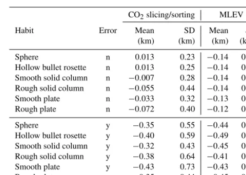
in-Table 4.Errors in retrieved cloud height for clouds with a
vari-ety of ice habits, using the CO2slicing/sorting and MLEV retrieval methods at a resolution of 0.5 cm−1. For the upper set of cases (er-ror=n), no errors were imposed on the retrieval, while for the lower set of cases (error=y) noise of 0.1 mW/(m2sr cm−1) and temper-ature bias of 0.1 K were imposed. The mean error (mean) and the standard deviation (SD) of the errors in retrieved cloud height are given.
CO2slicing/sorting MLEV
Habit Error Mean SD Mean SD
(km) (km) (km) (km)
Sphere n 0.013 0.23 −0.14 0.45
Hollow bullet rosette n 0.013 0.25 −0.14 0.54 Smooth solid column n −0.007 0.28 −0.14 0.45 Rough solid column n −0.055 0.44 −0.14 0.45
Smooth plate n −0.033 0.32 −0.13 0.46
Rough plate n −0.072 0.40 −0.12 0.45
Sphere y −0.35 0.55 −0.44 0.54
Hollow bullet rosette y −0.40 0.59 −0.49 0.59 Smooth solid column y −0.32 0.43 −0.45 0.54 Rough solid column y −0.38 0.64 −0.41 0.60
Smooth plate y −0.43 0.73 −0.43 0.56
Rough plate y −0.35 0.44 −0.45 0.57
homogeneous clouds in the first three rows. Error statistics for temporally varying clouds are typically intermediate be-tween those for the clouds that make them up. In the absence of errors, liquid-topped clouds have nearly identical statistics as the base dataset counterparts (i.e., diffuse clouds), while errors are slightly larger for CO2slicing/sorting when errors are imposed.
Sensitivity studies were also performed for simulations of various ice habits. Error statistics are compared in Table 4. For CO2slicing/sorting in the absence of errors, mean biases vary in sign and errors are slightly larger for non-spherical ice habits. However, statistics for MLEV are nearly identical. Furthermore, in the presence of even small errors, trends in error statistics with ice habit disappear.
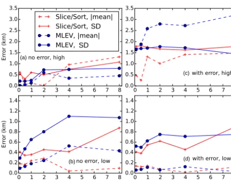
4.4 Dependence of cloud-height retrievals on resolution
(a)
(c)
(b) (d)
SD SD
Figure 6.Absolute value of mean error in retrieved cloud heights
and standard deviation in retrieved cloud heights as a function of instrument resolution for (a) low clouds (cloud bases below 2 km) with no imposed error,(b)high clouds (bases of 2 km and above) with no imposed error,(c)low clouds with imposed error, and (d) high clouds with imposed error. The errors imposed are 0.1 mW/(m2sr cm−1) noise in the cloudy-sky radiance and a bias of−0.1 K in the temperature profile used for the retrieval.
clouds (or close to 0); the figure shows the absolute values of the biases.
In the absence of error (left panels), retrieval errors in-crease gradually overall as resolution becomes coarser, from 0.1 to 8 cm−1. Furthermore, in the absence of error, overall MLEV is more accurate for high clouds, while CO2 slic-ing/sorting is more accurate for low clouds. In the pres-ence of imposed errors, behavior with resolution changes. For high clouds, magnitudes of mean biases increase rapidly with resolution for both methods between 0.5 and 1 cm−1, while standard deviations of errors remain constant. For low clouds, by contrast, mean biases remain fairly constant with resolution, while standard deviations of errors increase. Both represent increasing errors with coarsening resolution: for high clouds this is due to increasingly negative biases, while for low clouds this is due to increasingly variable er-rors. Overall, errors are larger for MLEV than for CO2 slic-ing/sorting when errors are imposed.
5 Discussion
5.1 Context with past studies
Mahesh et al. (2001) assume a variation of 3 % in the ratio of emissivities (ν)/(ν0)(i.e., error due to the assumption that emissivity is constant with wavenumber over the spec-tral region used). In their analysis, this source of uncertainty leads to uncertainty in retrieved cloud-base pressure of 5 to 13 mb (for a zenith angle of 45◦). Converting these to errors
in cloud-base height gives error estimates of 0.03 to 0.11 km for low clouds (bases of 0.1 to 1 km) and 0.14 km for a sin-gle high cloud at 2.1 km. In this work, we find that for high, thin clouds the variation in(ν)/(ν0)is closer to 5 %, re-sulting in biases of∼ −0.9 km for high clouds (above 2 km, for a zenith view). Furthermore, we estimate that errors in retrieved height due to other sources of model error are ap-proximately 0.2±0.3 km for low clouds and−0.2±0.4 km for high clouds. Thus this work expands on the error analysis of Mahesh et al. (2001) and indicates that retrieval errors for the CO2 slicing method applied to downwelling radiances are larger than previously predicted. However, errors in ac-tual cases will depend on the specific set of clouds sampled.
Holz et al. (2006) describe retrieval errors for CO2 slic-ing/sorting, CO2slicing (without sorting; not included here as a separate category), and MLEV. Note, however, that Holz et al. (2006) compare cloud-top height retrieved from upwelling (aircraft-based) infrared radiances (nadir view, 0.5 cm−1 instrument resolution) to cloud heights from li-dar measurements, whereas we compare cloud heights re-trieved from simulated downwelling radiances at the surface to known model cloud-base heights. Thus our results are not suited for detailed comparisons. However, some general ob-servations can be made. The results of Holz et al. (2006) sug-gest that CO2slicing/sorting is more accurate than MLEV for retrievals of optically thin clouds (τ <1.0) from measure-ments of upwelling radiance. This study indicates that, for downwelling radiances, the two are roughly equivalent and highly accurate, in the absence of errors, while in the pres-ence of errors accuracy is highly dependent on the source of error. As an example, this work shows that humidity bi-ases cause smaller errors for CO2 slicing/sorting than for MLEV; thus one explanation for the higher accuracy Holz et al. found for CO2 slicing/sorting could be errors in the humidity profiles they used. In addition, this work suggests that retrievals from upwelling radiance would benefit from a combined CO2slicing/sorting and MLEV method and can suggest implementation strategies based on expected error magnitudes. Finally, Holz et al. (2006) state that retrievals are challenging for clouds below 3 km using upwelling ra-diances. Since low clouds are retrieved most accurately us-ing downwellus-ing radiances, retrievals from surface-based in-frared spectrometers provide an important complement to re-trievals based on satellite measurements.
5.2 Dependence of cloud-height retrievals on cloud inhomogeneity and ice habit
physically thicker clouds having larger retrieval errors than physically thinner counterparts. Furthermore, for optically thinner clouds, the effective emitting height will be closer to the cloud middle, while for optically thick clouds, it will be closer to the cloud bottom. In keeping with this, clouds with optically thinner boundaries were found here to have larger retrieval errors compared to true cloud base. However, standard deviations of errors do not follow these trends when errors are imposed; this suggests that for real retrievals, the effects of cloud vertical inhomogeneity will be less important than other sources of error.
Varying the vertical distribution of cloud phase by plac-ing liquid at the cloud top is also expected to move the cloud effective emitting height upward, resulting in larger retrieval errors. However, this is only borne out here for CO2 slic-ing/sorting in the presence of imposed errors, for which er-rors are slightly larger (mean biases are 0.1 km higher and standard deviations of errors are 35 % larger). Converting from a uniformly mixed cloud to a liquid-topped cloud is expected to have a similar effect on retrieval errors as im-posing an optical depth that increases moving up through the cloud. Differences in statistics result because retrieved cloud heights are typically higher than for homogeneous mixed-phase clouds. (Note that these cases are all for clouds with bases below 2 km; for higher clouds this positive bias will work to counteract negative biases due to model errors.)
Error statistics for temporally varying clouds were found to be generally intermediate between those for the clouds that make them up, as expected. Thus we can expect that retrieved cloud heights for temporally varying clouds, or for clouds that vary horizontally within the instrument field of view, will be similar to the average cloud height to within expected retrieval error. Furthermore, an instrument such as the one proposed here can be used to measure temporal cloud homo-geneity and, using multi-angle measurements, cloud horizon-tal inhomogeneity (Rathke et al., 2002; Neshyba and Rathke, 2003). Because of their considerably smaller fields of view, knowledge of cloud inhomogeneity from surface-based surements would be a useful complement to satellite mea-surements.
Sensitivity studies were also performed for simulations of various ice habits. Differences are likely due to differences in the shape of the emissivity spectra for different habits. Re-call that the retrieval does not require any a priori knowl-edge or assumptions about ice habit but rather relies on the assumption that the emissivity is constant or varies slowly with wavenumber; thus ice habit affects cloud property re-trievals only inasmuch as it alters the frequency dependence of the cloud emissivity. Ice habits that result in spectrally flat-ter (i.e., closer to constant) emissivities should give more ac-curate results, while ice habits that result in more spectrally varying emissivities are expected to give less accurate results. When a smoothly varying emissivity is fitted, details about the variation of the emissivity, in combination with errors, will determine relative accuracy of the retrievals in a
man-ner that is difficult to predict. Here, error statistics for MLEV are found to be nearly identical for all ice habits. While er-rors are found to be slightly larger for non-spherical habits for CO2 slicing/sorting, in the presence of errors, trends in error statistics with ice habit disappear. Thus differences in statistics due to ice habit are likely to be negligible compared to sources of error.
5.3 Effects of errors on cloud-height retrievals
Figure 4 and Tables 1 and 2, presented in the results section, summarize errors for a resolution of 0.5 cm−1for a variety of sources of error. Table 1 summarizes error statistics for low clouds and Table 2 for high clouds. After screening out cases with cloud signal below 2.2 RU (see the columns indicated by “omit”), errors in retrieved cloud height (retrieved–true cloud-base height) are calculated for each remaining case. The mean error, representing the mean bias in retrieved cloud heights, and the standard deviation in the error are given in the table. The effect of model error, which is present even when no errors are imposed, is shown in the top row. Be-cause model error is present for all retrievals, the value in the table for each source of error is an overestimate. Cases were omitted when the RMS radiance difference for cloudy/clear-sky conditions (Robs−Rclr) was greater than a chosen thresh-old (2.2 RU). The threshthresh-old was chosen that eliminated all clouds with optical depths less than 0.25 and most with opti-cal depths less than 0.5 in the absence of imposed error (re-ferring back to Fig. 3a and b). In the presence of imposed error, more clouds are screened out for errors that reduce the cloudy-sky radiance or increase the clear-sky radiance, and vice versa. This typically eliminated less than about 20 low-cloud cases. For high clouds, about half (24–36 out of 67) of the clouds were screened out. High clouds emit less because they are colder and typically optically thinner than low clouds; furthermore they have a longer transmission path length through the atmosphere. Thus it seems likely that ap-plying such a threshold to real measurements will also screen out a greater proportion of high clouds (this was true in our dataset despite the fact there is no statistical difference be-tween the optical depths of high and low clouds). Tuning the threshold to a higher value will remove more low-signal cases, particularly high clouds.
as-similation sources. Thus, we assume the errors they found in ERA-Interim temperature and humidity profiles are simi-lar to what an autonomous spectrometer would experience in remote locations. Based on their temperature errors, we also performed retrievals for varying temperature errors: imposed errors were 1 K at 10 km, decreasing to−0.5 K at 2 km, and then increasing back to 1 K at 0.2 km. Because the tempera-ture at the surface will be measured and thus known very ac-curately, the imposed temperature error was reduced to 0 K at the surface. As shown in Tables 1 and 2, the effect of the varying temperature error based on Wesslen et al. (2014) was found to be roughly equivalent to the effect of a positive tem-perature bias of 0.2 K.
In addition to variable temperature errors, the effects of using temperature profiles in the retrieval that fail to capture temperature inversions were determined. Steep temperature inversions are common in polar regions that can be difficult to capture accurately from satellite. Such temperature inver-sions are included in the atmospheric profiles used here (see Cox et al., 2016). However, because measurements of surface temperature would accompany a surface-based instrument, extreme cases of error in profiling surface-based temperature inversions would be apparent by comparing the temperature measured near the instrument to the surface temperature in the assumed profile. In addition to surface-based inversions, aloft inversions are common, particularly in the presence of a cloud. To address the effects of poorly profiled temperature inversions, a set of retrievals was performed with temperature inversions removed from temperature profiles used in the re-trieval. Because the surface temperature would be known, the true value was replaced in the erroneous profile, and errors were allowed to increase over several layers to provide rea-sonable temperature differentials across the lower layers (the lowest model layers were set such that temperature differen-tials would not be more than 1 K for the lowest 1 km and not more than 5 K for the lowest 3 km). Resulting errors, shown previously in (Fig. 4g), affect CO2slicing/sorting more than MLEV, particularly for low clouds, and thus MLEV might be preferred for such cases. While surface-based temperature inversions that were not captured by reanalysis data could be identified and screened out from cloud-height retrievals, a better use would be to perform the retrievals to provide an important check on satellite and reanalysis data, correct-ing for the surface inversion to the extent possible given the known surface temperature and keeping in mind the elevated uncertainties. (In fact the instrument proposed here could also be used to improve temperature profiles, particularly for the lower troposphere, as similar instruments have been in use for such a purposes both from satellite and from the sur-face. Such improvements would thus improve the reanalysis results and therefore the input temperature to the cloud re-trievals.)
For water vapor, Wesslen et al. (2014) find mean errors to be typically positive and below 2 % for the first 3 km, after which they increase to 5 to 10 % from 4 to 8 km. For this
work we assume a relative bias of 3 % throughout the atmo-sphere. As for temperature, we assume the relative humidity will be measured to high accuracy at the surface and cor-rect the surface error to 0 %. This represents an underesti-mate of error in the upper atmosphere; however, most of the water vapor is in the lower atmosphere, where this represents an overestimate of error compared to Wesslen et al. (2014). Water vapor biases of±3 % at all heights were assumed to be roughly equivalent to the errors found by Wesslen et al. (2014) for ERA-Interim. For comparison, water vapor errors of 10 % were also calculated.
CO2errors are expected to be on the order of 0.5 %, based on the work of Alkhaled et al. (2008). Such CO2errors were found to produce negligible errors (not shown).
The final two rows of each table give estimates of com-bined sources of error, estimated as follows. First, we note that the effects of radiation bias and temperature bias are very similar (compare Fig. 4a, b, d, and e), so only one needs to be included; here we include radiation bias. We assume some cancellation of errors between radiation bias and tempera-ture and thus reduce the radiation bias to 0.15 RU, but we assume no cancellation between radiation bias and water va-por bias, pairing positive radiation bias with negative water vapor bias. Thus we simulate the combined error budget by imposing 0.2 RU for noise, 0.15 RU for radiation bias, and −3 % for water vapor. This is expected to be roughly equiva-lent to what is attained by combining errors in quadrature and is referred to in this work as combined error. In Fig. 4i, the combined errors are shown for both sets of calculations; there are approximately twice as many points on panel (i) as the other panels. For high clouds, errors for CO2slicing/sorting are highly variable and both positive and negative, while for MLEV they are strongly negatively biased. This occurs be-cause the sources of error tested do not be-cause strong positive biases in MLEV (only strong negative biases) regardless of the sign of the error.
found for retrievals of low clouds (for similar error levels). Instead, positive biases will generally be limited to the value shown by the line. For example, clouds with bases at 1 km will not generally be retrieved above 3.5 km. This means that when a high height is retrieved, the true cloud base is proba-bly high. Furthermore, when MLEV and CO2slicing/sorting disagree by more than 2 km, the true cloud-base is probably high. This allows accurate categorization of most clouds into low or high in the absence of strong temperature inversions and for well-characterized temperature inversions. As will be shown in more detail for a resolution of 4 cm−1, errors are strongly height dependent.
5.4 Hybrid methods
The fact that MLEV and CO2slicing/sorting show different susceptibilities to different sources of errors suggests that the best method is to use them in combination. This is reason-able as they use overlapping but distinct frequency regions. The exact details of how this is done will depend on the rel-ative magnitudes of errors for a given case, which in turn depends on knowledge of the atmospheric state. However, a few details are worth pointing out here.
Methods for combining MLEV and CO2 slicing/sorting are worth pursuing but are beyond the scope of this work. They could include combining them at the algorithmic level: for example, in a Bayesian analysis that determines the op-timal solution based on the intersection of the mean ±1 standard deviation probabilities for CO2slicing/sorting and MLEV. Otherwise, they could be combined post-retrieval by calculating a weighted combination of retrieved cloud heights for the two methods, where the weights depend on the uncertainty levels of the radiance, knowledge of the at-mospheric state, and retrieved heights. Regardless, how best to combine CO2 slicing/sorting and MLEV will depend on resolution and the magnitudes of sources of error and will require estimates of how errors are propagated into errors in retrieved cloud heights. The extra computational time taken for running both CO2slicing/sorting and MLEV is minimal because the most time-consuming computations are the cal-culations ofBc,tc, andRcfor each model layer, and this set of calculations is identical for the two methods (see step 1 for each method in Sects. 3.2 and 3.3).
In addition to the methods discussed here, an additional candidate for a hybrid cloud-height retrieval is one that re-lies on multi-angle sky views. Rathke et al. (2002) used a geometric method to retrieved cloud temperature from down-welling infrared radiance spectra measured using the Univer-sity of Puget Sound infrared spectrometer during the Surface Heat Budget of the Arctic (SHEBA) campaign (see Rathke et al., 2002, and references therein). This method was not compared with the MLEV and CO2 slicing/sorting meth-ods here for three reasons. First, they found RMS errors in cloud temperatures to be 5.1 K, whereas errors for a spec-tral method were found to be only 2.9 K (errors were
deter-mined by comparison to radiosonde temperature at the height determined to correspond to the cloud base by co-located lidar). Second, the multi-angle method is only appropriate for horizontally homogeneous clouds. Third, the method re-trieved cloud temperature and thus cannot distinguish be-tween heights above and below an inversion. However, such a method could help improve cloud-height determination for homogeneous clouds by incorporation into a hybrid method that makes primary use of the CO2 slicing/sorting method. For example, a multi-angle method could be used to improve knowledge of the spectral dependence of the emissivity. Ho-mogeneous clouds can be identified using a simple test; cases in which ln[1−Robs/Bc]is found to be inversely proportional to the cosine of the zenith viewing angle are identified as ho-mogeneous.
5.5 Effect of resolution on retrieval and choice of instrument characteristics
For CO2 slicing/sorting in the absence of errors, the mag-nitude of the mean bias in retrievals for high clouds in-creases with resolution, with the bias changing from∼0 km at 2 cm−1to−1 km at 4 cm−1(refer back to dashed red line in Fig. 6b, but note that the figures shows the absolute value of the mean bias). This is primarily due to the assumption that the emissivity is constant. As described previously, the vari-ation of the emissivity with wavenumber results in a mean bias of−0.9 at a resolution of 0.5 cm−1, but this bias is re-moved to a large extent by fitting the emissivity at high-signal points to a best-fit line and using the best-fit line to calculate a smoothly varying (linear rather than constant) emissivity. At resolutions coarser than∼2 cm−1, this correction is hindered by an insufficient number of points, and the bias reappears; note that a bias of−0.9 explains much of the magnitude of the bias shown for CO2 slicing/sorting in Fig. 6b at 4 and 8 cm−1. A similar increase is evident when errors are im-posed (dashed red line in Fig. 6c), but it occurs at a lower resolution (1 cm−1) and is overall larger due to the additional effect of the imposed errors.
pres-ence of errors, particularly for CO2slicing/sorting. Thus in the presence of errors, there is less benefit in using measure-ments at finer resolution.
On the basis of this resolution dependence, we explore the error budget at 4 cm−1. Comparing Figs. 4 and 5, we see the effect of reducing the resolution from 0.5 to 4 cm−1for high clouds is generally to lower the retrieved cloud base, in keeping with the enhanced mean bias shown in Fig. 6. For MLEV, at the coarser resolution, noise has a very large impact, resulting in retrieved heights that are below∼4 km regardless of true base height. Furthermore, for most error sources when MLEV is used, there are a number of cases for which errors are more than 2 km for clouds with bases near the surface. This occurs in part because MLEV has lost the ability to differentiate between clouds with bases above and below an inversion. (It is not clear why these errors are not apparent for combined errors, but note that the differences in local emissivity variances for choices above and below in-versions can be extremely small in the presence of errors for coarse resolution, resulting in high sensitivity to minor dif-ferences in errors.) Thus this analysis suggests that at a reso-lution of 4 cm−1and for noise≥0.2 RU, MLEV is of limited utility as a stand-alone method, although MLEV could pro-vide information in a hybrid CO2slicing/sorting and MLEV method. It is of interest to know whether these biases are born out in retrievals from real clouds; however, we are un-aware of any measurements of downwelling radiance cur-rently made at 4 cm−1resolution. Reducing the resolution of instruments currently deployed near active cloud profilers (li-dar and ceilometer) and comparing retrieved cloud heights is an interesting topic for future work. For CO2slicing/sorting, errors are large but the retrieval can still provide informa-tion. For example, most clouds with retrieved heights above 2.5 km can be reliably classified as high clouds. Overall, for CO2slicing/sorting (requiring a cloud signal of 2.2 RU), mean biases are−0.08 km for low clouds, with a standard de-viation in the error of 0.43 km, and mean biases are−1.3 km for high clouds, with standard deviations in the error of 1.5 km.
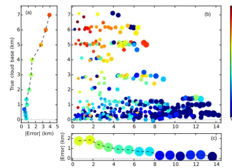
If the instrument characteristics assumed here (noise of 0.2 RU and bias of 0.2 RU) are difficult to achieve, it is also possible to screen out more optically thin cloud cases by in-creasing the cloud–signal threshold. The threshold of 2.2 RU (corresponding to optical depths below 0.25 to 0.5) removed many of the clouds with bases of 2 km and above; a larger threshold would exclude even more. Thus a stricter threshold would result in greater retrieval accuracy, at the cost of elim-inating more thin clouds from the analysis. In other words, retrieval accuracy is directly dependent on cloud signal and will be greater for thicker clouds. To better understand how the magnitude of retrieval errors depends on the threshold used for cloud detection, Fig. 7 shows cloud retrieval error at 4 cm−1for combined errors as functions of both cloud signal and cloud height. Thex axis for panels (b) and (c) is cloud signal, computed as the RMS difference between cloudy and
c
b
(a) (b)
(c)
Figure 7. (a)Binned means of the absolute values of errors in
re-trieved cloud heights (x axis) as a function of cloud-base height (yaxis), for estimated combined error budget (see text).(b) Abso-lute value of cloud-height retrieval error (given in color bar in km) as a function of cloud signal (root mean square of cloudy/clear-sky radiance) and true cloud-base height. A small random number is added to cloud-base heights in this panel to make them more easily distinguishable.(c)Binned means of the absolute values of errors as a function of cloud signal. Cloud heights were retrieved using CO2slicing/sorting from downwelling radiances at a resolution of 4 cm−1.
clear-sky radiance at the wavenumbers used in the retrieval, and they axis for panels (a) and (b) is true cloud base. In all panels, colors indicate the absolute value of cloud error; cloud errors are binned in panels (a) and (c). In panel (b), symbol size depends on cloud optical depth, illustrating the strong correlation between cloud signal and optical depth. Average absolute cloud-height errors decrease from 1.8 km at low cloud signal, to 0.2 km at high signal (panel c). The ab-solute values of cloud-height errors also generally decrease with decreasing cloud height (panel a). This is partly because higher clouds tend to have lower signal but also occurs inde-pendent of cloud signal.
The statistics of cloud-base heights used in this work are similar to those measured in the Arctic (see Cox et al., 2016, and references therein), with 79 % of the clouds below 2 km. Thus a surface-based spectrometer would be of the greatest benefit for retrieving the heights of low clouds, which are common in both the Antarctic (Bromwich et al., 2012; Ma-hesh et al., 2005) and the Arctic (Intrieri et al., 2002).
6 Conclusions