https://doi.org/10.5194/os-13-765-2017
© Author(s) 2017. This work is distributed under the Creative Commons Attribution 3.0 License.
Response to Filchner–Ronne Ice Shelf cavity warming in a coupled
ocean–ice sheet model – Part 1: The ocean perspective
Ralph Timmermann1and Sebastian Goeller1,a
1Alfred-Wegener-Institut Helmholtz-Zentrum für Polar- und Meeresforschung, Bremerhaven, Germany anow at: GFZ German Research Centre for Geosciences, Potsdam, Germany
Correspondence to:Ralph Timmermann (ralph.timmermann@awi.de) Received: 12 May 2017 – Discussion started: 19 May 2017
Revised: 18 August 2017 – Accepted: 21 August 2017 – Published: 21 September 2017
Abstract. The Regional Antarctic ice and Global Ocean (RAnGO) model has been developed to study the interaction between the world ocean and the Antarctic ice sheet. The coupled model is based on a global implementation of the Finite Element Sea-ice Ocean Model (FESOM) with a mesh refinement in the Southern Ocean, particularly in its marginal seas and in the sub-ice-shelf cavities. The cryosphere is rep-resented by a regional setup of the ice flow model RIMBAY comprising the Filchner–Ronne Ice Shelf and the grounded ice in its catchment area up to the ice divides. At the base of the RIMBAY ice shelf, melt rates from FESOM’s ice-shelf component are supplied. RIMBAY returns ice thickness and the position of the grounding line. The ocean model uses a pre-computed mesh to allow for an easy adjustment of the model domain to a varying cavity geometry.
RAnGO simulations with a 20th-century climate forcing yield realistic basal melt rates and a quasi-stable ground-ing line position close to the presently observed state. In a centennial-scale warm-water-inflow scenario, the model sug-gests a substantial thinning of the ice shelf and a local retreat of the grounding line. The potentially negative feedback from ice-shelf thinning through a rising in situ freezing tempera-ture is more than outweighed by the increasing water column thickness in the deepest parts of the cavity. Compared to a control simulation with fixed ice-shelf geometry, the coupled model thus yields a slightly stronger increase in ice-shelf basal melt rates.
1 Introduction
The mass flux from the Antarctic ice sheet to the South-ern Ocean is dominated by iceberg calving and ice-shelf basal melting. Until recently, it was assumed that iceberg calving was the dominant sink of Antarctic ice sheet mass, but ice-shelf basal melting is now estimated to outweigh all other processes (Depoorter et al., 2013; Rignot et al., 2013). Ice shelves have been shown to buttress the flow of outlet glaciers and ice streams (e.g. De Angelis and Skvarca, 2003; Dupont and Alley, 2005). Changes in ice-shelf thickness and grounding line location may therefore alter the discharge of ice grounded above floatation, and thus contribute to global sea level rise. The acceleration of mass loss from the Antarc-tic ice sheet since the 1990s (Rignot et al., 2011) has been attributed to enhanced ice-shelf basal melting and related ice-shelf thinning particularly in the Amundsen and Belling-shausen seas (Pritchard et al., 2012).
Figure 1.Schematic representation of the Filchner–Ronne Ice Shelf cavity, including cavity/shelf water circulation for the present-day Mode 1 melting/cold-water ice-shelf scenario.
freshwater flux on the Weddell Sea continental shelf, which is governed by sea ice formation, and thus largely determined by atmospheric forcing, is critical in allowing or preventing this transition in the melting mode. Observational evidence of warm pulses already arriving at the ice-shelf front (Dare-lius et al., 2016) indicates that this is a realistic scenario.
All model studies mentioned above assumed a static ice-shelf geometry even with simulated melt rates near the grounding line rising to almost 20 m year−1 (Timmermann and Hellmer, 2013). To overcome this deficiency and study ice-shelf–ocean interaction in a warming climate in a con-sistent way, we coupled the Finite Element Sea-ice Ocean Model (FESOM) to a regional setup of the ice flow model RIMBAY (Thoma et al., 2014) and forced the coupled model with output from HadCM3 that has been obtained for present-day climate and the A1B scenario (Collins et al., 2011). This paper describes the coupling procedure and re-ports on the solutions we found for a suite of technical chal-lenges (Sect. 2). A 250-year-long coupled model run with climate-projection forcing serves as the reference simula-tion and is compared to control experiments with (i) con-tinuous present-day forcing and (ii) static ice-shelf geometry (Sect. 3). The focus of the analysis here is on processes and sensitivities in the sub-ice-shelf cavity. Ice dynamics and ice sheet mass balance will be discussed in the companion pa-per (Part 2: The ice pa-perspective; Goeller and Timmermann, 2017).
2 Regional Antarctic ice and Global Ocean model (RAnGO)
2.1 Overview
RAnGO combines a regional model of the Antarctic ice sheet with a global ocean model. The coupled system consists of a global configuration of FESOM (Timmermann et al.,
Figure 2. Horizontal resolution of RAnGO’s ocean component. Note the nonlinear colour scale.
2012), and a regional setup of the Revised Ice Model Based on frAnk pattYn (RIMBAY; Thoma et al., 2014). While the FESOM domain covers the world ocean including the sub-ice-shelf cavities in the Southern Ocean, the RIMBAY setup comprises the FRIS and the relevant catchment basin up to the ice divides. The interface between the two models is the FRIS base (Fig. 1). All other ice shelves are modelled with fixed geometry. As for the stand-alone model runs of Hellmer et al. (2012), the coupled model is forced by atmospheric out-put from the HadCM3 climate model.
2.2 The ocean component: FESOM
FESOM is a primitive-equation hydrostatic ocean model that is solved on a horizontally unstructured mesh (Wang et al., 2014). It comprises a dynamic–thermodynamic sea ice model (Danilov et al., 2015). The ice-shelf component (Timmermann et al., 2012) goes back to the Hellmer and Ol-bers (1989) three-equation model of ice-shelf–ocean inter-action with a velocity-dependent parameterization of bound-ary layer heat and salt fluxes according to Holland and Jenk-ins (1999).
Ice model domain
Figure 3.Antarctic ice sheet with coast and grounding lines (black) and the ice divides (green and blue) from Antarctica’s Gamburtsev Province Project (AGAP). The green lines indicate the RIMBAY model domain in this study.
An early version of RTopo-2 (Schaffer et al., 2016) has been used to derive ocean bathymetry and the ice-shelf draft and grounding lines for all cavities with fixed geometry. With the present-day ice-shelf configuration for FRIS, the FESOM mesh comprises a total of ≈2.6×10⁶ nodes, 1.1×10⁵of which are surface nodes (where the term surface equally refers to open ocean and ice-shelf base). The model is run with a default time step of 90 s owing to the very fine horizon-tal resolution along the FRIS grounding line and a minimum sigma layer thickness of just over 2 m. For several situations with eddies running into shallow sections of the FRIS cav-ity, it turned out to be necessary to decrease the ocean model time step to 4 s.
2.3 The ice component: RIMBAY
RIMBAY (Thoma et al., 2014) is a three-dimensional ther-momechanical multi-approximation ice-shelf/sheet model going back to the ice flow model of Pattyn (2003). Within the RAnGO experiments, the ice model domain comprises the FRIS and its upstream catchment area of grounded ice, confined by the surrounding ice divides (Fig. 3). Ice ve-locities are calculated following the hybrid approach which combines the shallow-ice and the shallow-shelf approxima-tions. A basal friction correction at the grounding line after Feldmann et al. (2014) ensures a smooth transition between grounded and floating ice and thus a realistic grounding line migration.
The ice model is run at a horizontal resolution of 10 km with 41 terrain-following sigma layers and a time step of 0.1 years. Bedmap2 (Fretwell et al., 2013) data are used for bedrock topography and initial ice thickness. Since Bedmap2
Figure 4.RAnGO initialization and coupling scheme. The red ar-row indicates the most time-consuming element of the model cou-pling.
is also the source for the Antarctic ice and bedrock re-lief in RTopo-2, all topographies are fully consistent within RAnGO.
2.4 Model spinup and coupling
First, we perform a 1000-year stand-alone RIMBAY simula-tion. This ice model spinup is forced by present-day surface temperatures (Comiso, 2000), accumulation rates (Arthern et al., 2006) and geothermal heat flux (Shapiro and Ritzwoller, 2004). Basal melt rates are parameterized according to Beck-mann and Goose (2003). As a result, ice dynamics are in a quasi-stationary steady state and ice thickness, ice velocity, and grounding line position match current observations very well. Additional figures and a thorough discussion of the ice model spinup are presented in our companion paper (Part II: the ice perspective; Goeller and Timmermann, 2017).
With thisRIMBAY present-daycavity geometry, we inte-grate FESOM for 21 years (1930–1950) using atmospheric forcing from the 20th-century simulation of the HadCM3 cli-mate model. Annual mean basal melt rates for FRIS from the last year (1950) are then transferred back to RIMBAY, which starts the RAnGO coupled model loop (Fig. 4).
For each of the cycles within the coupled RAnGO sys-tem, FRIS basal melt rates averaged over yearNare obtained from FESOM and passed to RIMBAY, which is then stepped forward for that same yearN. From the simulated ice draft and grounding line location at the end of RIMBAY yearN, a new cavity geometry is derived and an updated FESOM mesh is generated. FESOM’s prognostic variables are pro-jected onto the new mesh (details below), and FESOM is then integrated over yearN+1. Basal melt rates are aver-aged over FESOM yearN+1 and passed to RIMBAY, and the cycle repeats itself with RIMBAY running yearN+1.
Figure 5. Precomputed and actual FESOM mesh in the Weddell Sea/FRIS sector: blue triangles indicate open ocean; green triangles indicate ice-shelf cavities in the RAnGO geometry for simulated year 2000 (i.e. at the end of the 20th-century spinup). Red triangles refer to elements that have been created in the initial mesh but are removed for the year 2000 geometry because they were found to be covered with grounded ice (potential ocean mesh in a warming scenario).
grounding line location, and melt rate patterns are small for each coupling time step indicates that this coupling strategy is adequate.
2.5 Dynamic FESOM mesh modification
Adjustment of the model domain to a varying ice-shelf ge-ometry is a natural part of RIMBAY and is rather straightfor-ward to implement for a finite-difference ocean model with a land–sea mask. For FESOM, the computational mesh only exists in the ocean and has to satisfy certain criteria in order to ensure numeric stability and efficiency. For stand-alone FESOM applications (e.g. Timmermann et al., 2012) we use an iterative method to generate surface meshes in which the size of triangles smoothly varies according to the desired resolution, while at the same time triangles approximate the ideal of being equilateral as well as possible. For a mesh with about 105surface nodes, the algorithm takes about 2 days to converge – which clearly prevents it from being used as part of a coupling interface.
To reduce the mesh generation overhead, we generated an initial surface grid that covers the full RTopo-2 ocean (blue and green triangles in Fig. 5) plus all ice around FRIS that is grounded on bedrock deeper than 100 m below sea level (red triangles in Fig. 5). This criterion to define the “poten-tially ungrounding” area adjacent to the currently floating ice shelf proves to be well on the safe side for any ground-ing line movement in our coupled model runs. Mesh reso-lution along the present-day grounding line and in the
po-tentially ungrounding area is about 1 km to describe ground-ing line migration as smoothly as possible. For each topog-raphy/cavity geometry to be run with RAnGO, the coupler removes all grid nodes that are covered by grounded ice. The remaining ocean grid nodes are renumbered consecutively. The full three-dimensional grid is then created from this new surface mesh, with the terrain-following vertical coordinate easily adjusting to any change in water column thickness due to a varying ice-shelf draft.
During this procedure, the vast majority of finite element mesh nodes keep their position (despite being renumbered), so that no horizontal interpolation is necessary for the ocean state variables outside the immediate vicinity of the ground-ing line. This makes it much easier to ensure the conser-vation of heat and salt. Wherever new ocean (i.e. cavity) nodes are created, ocean temperature, salinity, and sea sur-face height are taken from the nearest existing neighbour grid node. Again, the small variations per coupling step make this simple “no-flux” approach justified.
2.6 Computational load
Coupling has been implemented in an “offline” way with RIMBAY and the RAnGO coupler running on local servers and FESOM relying on a massively parallel supercomputing system. Given that (1) model output is in any case transferred to local disks for postprocessing and analysis and that (2) the updated mesh configuration files are comparatively small, the overhead arising from the file transfer necessary in our offline approach is negligible.
To run a typical model year with the current configuration of RAnGO requires about 7 h on 528 CPUs for FESOM, less than 10 min for RIMBAY, and almost 2.5 h for the coupling procedures. Within the coupler, more than 90 % of the time is spent on the construction of the three-dimensional, tetrahe-dral mesh from the updated surface grid. A more efficient al-gorithm that starts from the existing three-dimensional mesh and only applies corrections where necessary is currently be-ing developed.
2.7 Experiments
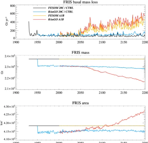
Figure 6. Time series of annual-mean basal melt rate, ice-shelf mass, and ice-shelf area for FRIS in fixed-geometry FESOM exper-iments with 20th century (black line) and A1B (yellow line) forcing and in RAnGO experiments for the 20th century (blue line) and the A1B scenario (red line).
has been performed twice repeating the HadCM3 1900–1999 forcing.
Next to the coupled RAnGO simulation launched from the end of 1950, an uncoupled FESOM experiment with the RIMBAY present-day cavity geometry prescribed has been conducted. Like its RAnGO counterpart, this experiment starts with a FESOM 20C simulation and splits into a FE-SOM A1B and aFESOM CTRLbranch at the beginning of the 21st century.
3 Results
3.1 Ice-shelf basal melt rates and hydrography 3.1.1 Present-day climate in FESOM and RAnGO Time series of simulated mean basal melt rates in theFESOM 20C andRAnGO 20Csimulations (black and blue lines in Fig. 6) indicate that ice-shelf–ocean interaction approaches a quasi-steady state within less than a decade after the ini-tialization with a relatively warm water mass in the FRIS cavity. Mean basal mass loss over the period 1950–1999 amounts to 87 Gt year−1in the fixed-geometry FESOM ex-periment and to 93 Gt year−1 in the fully coupled RAnGO model run. Both are well within the range of observational estimates (e.g. 50±40 Gt year−1, Depoorter et al., 2013, vs. 155±35 Gt year−1, Rignot et al., 2013); the difference
be-tween the two experiments is much smaller than the (mod-elled) interannual variability.
Maximum melt rates for present-day climate (Fig. 7a) are about 5 m year−1and occur in the deepest parts of the cavity close to the grounding lines of Support Force Glacier and Foundation Ice Stream, where the ice base reaches 1100 and 1400 m below sea level, respectively (Fig. 7d), and the in situ freezing point is about 1 K below the surface freezing point. Melt rates between 3 and 5 m year−1are suggested for Evans and Rutford Ice streams in the western sector of Ronne Ice Shelf, which is consistent with estimates based on ice flux divergence (Joughin and Padman, 2003).
An extended area of marine ice formation is suggested north of (i.e. downstream from) the Henry and Korff Ice rises. While this pattern is consistent with the observed locations of marine ice (Lambrecht et al., 2007), accretion rates in most of the refreezing area are smaller than in the estimates of Joughin and Padman (2003).
Two additional hot spots of marine ice formation (at rates exceeding 1.0 m year−1) are associated with the outflow of Ice Shelf Water (ISW) in the Filchner and Ronne troughs. For Filchner Trough, this is again consistent with Joughin and Padman (2003), although their data and the marine ice thick-nesses observed by Lambrecht et al. (2007) suggest a more pronounced freezing pattern on the western side. For the western side of Ronne Trough, marine ice formation along the coast is consistent with the sub-ice circulation, as sug-gested by Nicholls et al. (2004).
Modelled present-day cavity geometry agrees well with the location of grounding lines in Bedmap2, except for the three narrow ice streams feeding the western sector of Ronne Ice Shelf. Due to small ice thickness and bedrock gradients, the grounding line positions in this area are highly sensitive to ice thickness changes during the RIMBAY spinup. A strin-gent validation of modelled FRIS topography is provided in Part II of this paper.
3.1.2 FESOM and RAnGO A1B projections
Figure 7.Ten-year mean basal melt rates in theRAnGO 20Cexperiment for 1990–1999(a), inRAnGO A1Bfor 2190–2199(b), and in
FESOM A1Bfor 2190–2199(c). Corresponding ice-shelf drafts from theRAnGO 20C/A1Bsimulation for 1995(d)and 2195(e), and in the
RIMBAY present-daygeometry(f). Abbreviations indicate the locations of Support Force Glacier (SF), Foundation Ice Stream (FI), Evans Ice Stream (EI), Rutford Ice Stream (RI), Henry Ice Rise (H), Korff Ice Rise (K), Ronne Trough (RT), and Filchner Trough (FT). Coloured areas represent modelled cavity geometries. Black lines denote coast and grounding lines from RTopo-2.
The strongest increase in basal melt rates occurs be-tween 2050 and 2070. Like in the experiments of Hellmer et al. (2012) and Timmermann and Hellmer (2013), this is caused by a flow of Modified Warm Deep Water (MWDW) onto the continental shelf and into the sub-ice-shelf cav-ity (Fig. 8). In contrast to the former FESOM experiments, which adopted a water column thickness of about 200 m southwest of Henry Ice Rise from RTopo-1 (Timmermann et al., 2010), slightly thicker ice in RIMBAY and a better rep-resentation of bottom topography in the RAnGO (FESOM) simulations discussed here lead to a water column thickness of only 120 m (90 m) in the channel, and thus prevent a rapid spreading of warm water into the Ronne cavity.
The change in hydrography in the second half of the 21st century is very similar between the coupled RAnGO simula-tion and the uncoupled FESOM experiment with fixed cavity geometry (not shown). Area-mean basal melt rates in FE-SOM A1B follow the RAnGO A1B evolution very closely until about 2050 (top panel in Fig. 6). Differences increase within a few decades after the onset of cavity warming, with
the fixed-geometry melt rates always staying below their RAnGO counterparts. With 418 Gt year−1forFESOM A1B, the mean basal mass loss over the period 2190–2199 is about 20 % lower than in the coupled RAnGO simulation. The distribution of melt rates, however, is very similar between RAnGO A1BandFESOM A1B(Fig. 7b, c).
Figure 8. (a)Simulated bottom temperature for 2053 and 2071 in theRAnGO A1Bexperiment. Panel(b)indicates the corresponding points in time on the time series of annual-mean basal mass loss.
of water getting in touch with the ice-shelf base along the ice front.
3.1.3 FESOM and RAnGO 20C control experiments In contrast to the regime shift suggested by theA1B experi-ments, the control runs with a perpetual 20th-century forcing (black and blue lines in Fig. 6) preserve the “cold-water ice shelf” state of the original FESOM 20C and RAnGO 20C simulations with only little change in the distribution and area-average of basal melt rates. The rapid cavity warming caused by an inflow of MWDW does not occur in these sim-ulations.
3.2 Ice-shelf thickness, area, and mass 3.2.1 RAnGO A1B experiments
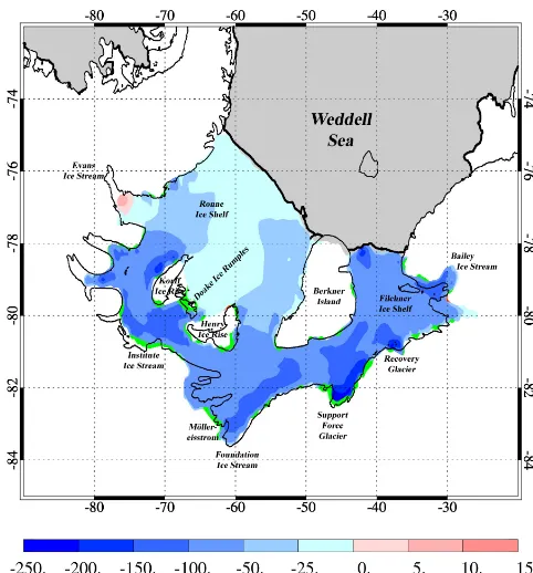
Owing to the increasing basal melt rates in the A1B scenario, FRIS in theRAnGO A1Bsimulation continuously loses mass from 2050 onwards (Fig. 6, middle panel). Between the 1990s and the 2190s, FRIS mass decreases by 1.4×10⁴Gt (i.e. 6.1 %). Consistent with the location of the highest melt rates, the strongest thickness decrease occurs at the inflow of Support Force Glacier (Fig. 9). At the maximum, ice-shelf draft (thickness) is reduced by 225 (286) m between 1995 and 2195 here. This is also one of the few locations with a substantial grounding line retreat (green areas in Fig. 9). De-spite the fact that melt rates (and the melt rate increase) are
of similar magnitude at the floating parts of Foundation Ice Stream, ice draft reduction does not exceed 150 m and the grounding line remains stable there. This discrepancy will be analysed in Part II of this paper.
Other locations of substantial grounding line retreat are at the Möllereisstrom, the Institute Ice Stream, and at the Henry and Korff Ice rises; the Doake Ice Rumples become detached from the ice-shelf base. The area of floating ice (Fig. 6, lower panel) increases by 1.15×10¹⁰m2(i.e. 2.8 %).
While ice-shelf thickness trends are small for the northern sector of Ronne Ice Shelf, a substantial thinning is also found at the Filchner Ice Shelf front. This is associated with the increasing rate of “Mode 3” melting during the increasingly long summer season (Fig. 7c), and thus reflects the impact of a decreasing sea ice coverage/increasing summer sea surface temperature on basal melting near the ice-shelf front.
3.2.2 Present-day climate control experiment
Figure 9.Simulated ice draft change (m) for FRIS from 1995 to 2195 in theRAnGO 20C/A1Bexperiment. Note the nonlinear colour scale. Green colour indicates areas of originally grounded ice that becomes afloat. Two small red patches represent areas of float-ing ice that becomes grounded. Thin (thick) black lines indicate coast/grounding lines (ice-shelf fronts) from RTopo-2.
a gradual FRIS thickness loss during the first decade of the 21st century (Paolo et al., 2015) this might well be consistent with the true current situation. In any case, this model back-ground variability is very small compared to the divergence between the two simulations after≈2070.
3.3 Thickness–melt-rate feedback
As has been discussed in Sect. 3.1.2, simulated basal melt rates increase by roughly a factor of 6 between the 1990s and the 2190s in theRAnGO A1BandFESOM A1Bsimulations. Taking a more quantitative view, we find an increase factor of 6.1 forRAnGO A1Bvs. only 5.4 forFESOM A1B. We also note that the area-mean melt rate inRAnGO A1Bis always higher than inFESOM A1B(Fig. 6). Given that a reducing ice draft implies a rising in situ freezing temperature and thus a reducing melt potential for any warm water mass flowing into the cavity, this is not necessarily an obvious result – instead it would have appeared plausible to assume that a reducing ice thickness would reduce (not increase) the basal melt rate in a warming scenario like the one discussed in this study. In this section, we will therefore look into the processes that lead to an increased melt for a thinning ice shelf.
From the RAnGO and FESOM melt rate maps for the 2190s (Fig. 7b, c) a systematic change introduced by the
tran-sition from a fixed geometry to a coupled model is not obvi-ous. A map of the difference between the two fields (Fig. 10, panel a) reveals that in many places with a retreating ground-ing line, an increased melt in newly ungrounded areas is at least partly compensated by reduced melt in areas along the old grounding line location. Even in this warm-water-inflow scenario, ice-shelf–ocean interaction in many places still ap-pears to fully extract the heat content of water getting in touch with the ice base near the grounding line, so that a shift in the grounding line position merely shifts the location of melt rate maxima, but does not increase total melt.
A more substantial and largely unbalanced melt rate in-crease is found (1) along the ice-shelf front and (2) at loca-tions with a substantial increase in water column thickness. Along the ice-shelf front, increasing melt rates in the A1B scenario lead to a reduction of thickness (only) in the coupled model, reducing its function as a dynamic barrier. Second, reducing ice draft close to the grounding lines leads to an increasing water column thickness below still deep-drafted ice, even if the grounding line position remains unchanged or grounding line migration is very small. In several loca-tions that have already been under the floating ice shelf in the present-day situation, up to 90 % of the water column thickness found at the end of theRAnGO A1Bsimulation are due to ice-shelf thinning (Fig. 10, panel b). Even though the water mass properties change only very little between FE-SOM A1BandRAnGO A1B (Fig. 11), the increased water column thickness in the coupled model allows for a trans-port of warm water to the deepest parts of the cavity more easily. This is most notable at the estuaries of the Recovery and Support Force glaciers, but also to the north of Bailey Ice Stream. At Support Force Glacier, the increasing melt rates in the A1B scenario lead to a reduced ice-shelf thickness and an increased slope of the ice-shelf base directly off the grounding line (Fig. 11). The latter causes 2195 annual mean along-slope ocean current velocities at the ice-shelf base to increase from about 5 cm s−1inFESOM A1Bto a maximum of 15 cm s−1inRAnGO A1B, reinforcing stronger melt rates in this area and thus forming a positive feedback loop. Some of this increased melting is compensated by a reduced melt-ing in adjacent areas, but the residual remains positive, so that together with the increased melting along the ice front, total ice-shelf basal mass loss in the coupled model increases slightly more than in the fixed-geometry case.
3.4 Lessons from initial adjustment
A striking feature in the time series of Fig. 6 is the sudden reduction of FRIS mass and area from 1950 to 1951, i.e. with the first coupling step. What appears as a big discontinuity merely represents 2.7 % of the original ice-shelf mass and 1.0 % of ice-shelf area. Nevertheless, this event deserves a closer look.
Figure 10. (a)Difference in simulated mean melt rates for the period 2190–2199 in coupled and fixed-geometry simulations (RAnGO minus FESOM).(b) Increase in water column thickness (wct) fromFESOM A1Bto RAnGO A1Brelative to theRAnGO A1B2195 state. For example, an increase of 90 % at a given location means that 90 % of the water column thickness found in 2195 has been created by ice-shelf thinning.
Figure 11. Annual mean potential temperature sections for 2195 below Filchner–Ronne Ice Shelf in RAnGO A1B (a) and FESOM A1B (b). Colours on top of the ice-shelf base indicate annual mean basal melt rates. The red lines in the maps indicate the location of the section.
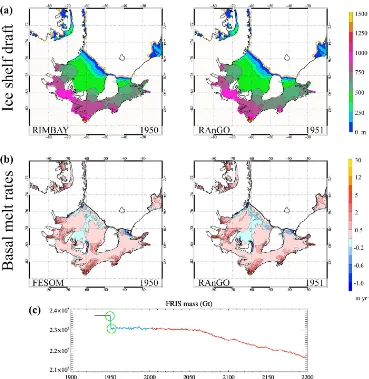
RAnGO, i.e. the first year in which RIMBAY is forced with basal melt rates from FESOM. The top left panel in Fig. 12 thus shows the FRIS thickness distribution at the end of the 1000-year RIMBAY spinup with Beckmann and Goose (2003) melt rates, representing theRIMBAY present-daygeometry introduced above. Using this ice thickness dis-tribution, FESOM has been integrated with a fixed cavity ge-ometry for 21 years. Annual-mean melt rates from the last year of this simulation (Fig. 12, bottom left panel) are fed back to RIMBAY as part of the first communication step of the coupled model. Ice thickness distribution after this firstRAnGOyear (Fig. 12, top right panel) shows that com-pared to the RIMBAY present-day geometry, ice thickness
Figure 12. (a)Simulated ice-shelf draft for 1950 and 1951.(b)Simulated basal melt rates averaged over the same years.(c)Time series of FRIS mass with green circles indicating the relevant points in time. The area covered in colours represents the modelled ice-shelf area; black lines indicate coastlines derived from RTopo-2.
4 Discussion and conclusions
We have presented the coupled ice sheet–ice shelf–ocean model RAnGO which is focused on the Filchner–Ronne Ice Shelf (FRIS) and the grounded ice in its catchment basin. For present-day climate, the model yields ice-shelf basal melt rates, ice thickness, and grounding line location in good agreement with observations.
As the reference simulation, we used a coupled model run forced with A1B scenario data from the HadCM3 climate model. Similar to the experiments of Hellmer et al. (2012) and Timmermann and Hellmer (2013), a substantial increase in FRIS basal melt rates during the 21st and 22nd centuries occurs as a response to inflowing MWDW in this simulation. This event does not occur in two control simulations (cou-pled/uncoupled) with a perpetual 20th-century forcing from the same climate model and can thus clearly be attributed to the climate scenario/forcing data used.
Basal mass loss in the coupled A1B simulation increases by a factor of 6 between the simulated 1990s and the pro-jected 2190s; maximum melt rates near the grounding line increase from 4 to 15 m year−1. Increasing melt rates lead to a thinning of the ice shelf between the present-day situa-tion and the end of the 22nd century, especially in the deepest parts along (but not directly at) the grounding line. Maximum thickness loss in the coupled model is 280 m and occurs near the grounding line of Support Force Glacier. Grounding line migration does not exceed a distance of about 20 km. A more detailed discussion of dynamics in the various ice streams is provided in Part II of this paper.
switching from Beckmann and Goosse (2003) melt rates to FESOM melt rates as a boundary condition for RIMBAY at the end of the ice model spinup; it is also true for the strongly increased melt rates projected for the end of the 22nd century, which are very similar for theRAnGO A1Band theFESOM A1Bcavity geometries despite an ice thickness difference of up to 280 m (i.e. almost 25 %). We conclude that parameter-izing ice-shelf basal melt rates as a function of ice thickness, like in the widely used scheme suggested by Beckmann and Goosse (2003), is not necessarily a good approximation to the governing processes.
Although the basal melt rates are not identical between the coupled and uncoupled simulations, our results indicate that on a timescale of up to 2 centuries, many aspects of ice-shelf–ocean interaction at Filchner–Ronne Ice Shelf can be addressed with a fixed ice-shelf geometry even in a changing climate. The long-term trend with basal mass loss increas-ing by roughly a factor of 6 in the A1B scenario is fully consistent between the coupled and uncoupled simulations. Year-to-year variability of basal mass loss is very similar be-tween the coupled and uncoupled simulations both for A1B scenario forcing and in the 20th-century control runs.
A more quantitative comparison between theRAnGO A1B experiment and the control simulation with A1B forcing but fixed cavity geometry (“FESOM A1B”) reveals that the in-crease in basal melt rate as a response to ice-shelf cavity warming is enhanced by about 12 % in the coupled simu-lation. The reduced melt potential due to the rising freez-ing point in areas with decreasfreez-ing ice thickness in the cou-pled simulation is clearly outweighed by the increasing wa-ter column thickness and the increasing ice base slope, both of which cause a more efficient heat transfer and thus higher melt rates in the deepest part of the cavity. We conclude that using a fixed-geometry ice-shelf–ocean model tends to atten-uate rather than exaggerate the response of ice-shelf basal melt rates to ocean climate warming. The long-term evo-lution of ice–ocean interaction at the shores of Antarctica under progressing climate warming and thus the projection of Antarctica’s contribution to future global sea level rise clearly demand an appropriate consideration of coupled pro-cesses in regional and global climate models.
Code availability. Codes for RIMBAY and FESOM are available from the authors upon request.
Author contributions. RT set up FESOM, developed and imple-mented the RAnGO coupling scheme, conducted the experiments, and prepared most of the paper. SG set up the RIMBAY model, provided the RIMBAY interface to the coupling routines, and con-tributed to the preparation of the paper.
Competing interests. The authors declare that they have no conflict of interest.
Acknowledgements. We would like to thank Klaus Grosfeld, Hartmut Hellmer, Rachael Mueller, Dmitry Sidorenko, and Qiang Wang for helpful discussions; Sina Löschke for supplying the illustration of Weddell Sea continental-shelf processes; Wolf-gang Cohrs, Herbert Liegmahl, Natalja Rakowsky, Malte Thoma, and Chresten Wübber for maintaining excellent computing facil-ities at AWI; and the two anonymous reviewers for their careful reading and helpful suggestions. Frank Schnaase created the scripts for combining sub-ice temperature sections with basal melt rate profiles. We thank the North German Supercomputing Alliance (HLRN) for providing the computer resources required to run FESOM and RAnGO over several hundreds of years. Funding by the Helmholtz Climate Initiative REKLIM (Regional Climate Change), a joint research project of the Helmholtz Association of German Research Centres (HGF), has been indispensable for this study and is gratefully acknowledged.
The article processing charges for this open-access publication were covered by a Research
Centre of the Helmholtz Association. Edited by: Andreas Sterl
Reviewed by: two anonymous referees
References
Arthern, R. J., Winebrenner, D. P., and Vaughan, D. G.: Antarc-tic snow accumulation mapped using polarization of 4.3-cm wavelength microwave emission, J. Geophys. Res.-Atmos., 111, D06107, https://doi.org/10.1029/2004JD005667, 2006. Beckmann, A. and Goosse, H.: A parameterization of ice shelf–
ocean interaction for climate models, Ocean Model., 5, 157–170, 2003.
Collins, M., Booth, B. B. B., Bhaskaran, B., Harris, G. R., Murphy, J. M., Sexton, D. M. H., and Webb, M. J.: Climate model er-rors, feedbacks and forcings: a comparison of perturbed physics and multi-model ensembles, Clim. Dynam., 36, 1737–1766, https://doi.org/10.1007/s00382-010-0808-0, 2011.
Comiso, J. C.: Variability and trends in Antarctic surface temperatures from in situ and satellite infrared measure-ments, J. Climate, 13, 1674–1696, https://doi.org/10.1175/1520-0442(2000)013<1674:VATIAS>2.0.CO;2, 2000.
Danilov, S., Wang, Q., Timmermann, R., Iakovlev, N., Sidorenko, D., Kimmritz, M., Jung, T., and Schröter, J.: Finite-Element Sea Ice Model (FESIM), version 2, Geosci. Model Dev., 8, 1747– 1761, https://doi.org/10.5194/gmd-8-1747-2015, 2015.
Darelius, E., Fer, I., and Nicholls, K. W.: Observed vulner-ability of Filchner-Ronne Ice Shelf to wind-driven inflow of warm deep water, Nature Communications, 7, 12300, https://doi.org/10.1038/ncomms12300, 2016.
Depoorter, M. A., Bamber, J. L., Griggs, J. A., Lenaerts, J. T. M., Ligtenberg, S. R. M., van den Broeke, M. R., and Moholdt, G.: Calving fluxes and basal melt rates of Antarctic ice shelves, Na-ture, 502, 89–92, https://doi.org/10.1038/nature12567, 2013. Dupont, T. K. and Alley, R. B.: Assessment of the importance of
ice-shelf buttressing to ice-sheet flow, Geophys. Res. Lett., 32, L04503, https://doi.org/10.1029/2004GL022024, 2005. Feldmann, J., Albrecht, T., Khroulev, C., Pattyn, F., and Levermann,
A.: Resolution-dependent performance of grounding line motion in a shallow model compared with a full-Stokes model accord-ing to the MISMIP3d intercomparison, J. Glaciol., 60, 353–360, 2014.
Fretwell, P., Pritchard, H. D., Vaughan, D. G., Bamber, J. L., Bar-rand, N. E., Bell, R., Bianchi, C., Bingham, R. G., Blanken-ship, D. D., Casassa, G., Catania, G., Callens, D., Conway, H., Cook, A. J., Corr, H. F. J., Damaske, D., Damm, V., Ferracci-oli, F., Forsberg, R., Fujita, S., Gim, Y., Gogineni, P., Griggs, J. A., Hindmarsh, R. C. A., Holmlund, P., Holt, J. W., Jacobel, R. W., Jenkins, A., Jokat, W., Jordan, T., King, E. C., Kohler, J., Krabill, W., Riger-Kusk, M., Langley, K. A., Leitchenkov, G., Leuschen, C., Luyendyk, B. P., Matsuoka, K., Mouginot, J., Nitsche, F. O., Nogi, Y., Nost, O. A., Popov, S. V., Rignot, E., Rippin, D. M., Rivera, A., Roberts, J., Ross, N., Siegert, M. J., Smith, A. M., Steinhage, D., Studinger, M., Sun, B., Tinto, B. K., Welch, B. C., Wilson, D., Young, D. A., Xiangbin, C., and Zirizzotti, A.: Bedmap2: improved ice bed, surface and thickness datasets for Antarctica, The Cryosphere, 7, 375–393, https://doi.org/10.5194/tc-7-375-2013, 2013.
Goeller, S. and Timmermann, R.: Response to Filchner-Ronne Ice Shelf cavity warming in a coupled ocean–ice sheet model – Part 2: The ice perspective, to be submitted to The Cryosphere, 2017. Hellmer, H. H. and Olbers, D.: A two-dimensional model for the thermohaline circulation under an ice shelf, Antarct. Sci., 1, 325– 336, 1989.
Hellmer, H. H., Kauker, F., Timmermann, R., Determann, J., and Rae, J.: Twenty-first-century warming of a large Antarctic ice-shelf cavity by a redirected coastal current, Nature, 485, 225– 228, https://doi.org/10.1038/nature11064, 2012.
Holland, D. M. and Jenkins, A.: Modelling thermodynamic ice-ocean interactions at the base of an ice shelf, J. Phys. Oceanogr., 29, 1787–1800, 1999.
Jacobs, S. S., Hellmer, H. H., Doake, C. S. M., Jenkins, A., and Frolich, R. M.: Melting of ice shelves and the mass balance of Antarctica, J. Glaciol., 38, 375–387, 1992.
Joughin, I. and Padman, L.: Melting and freezing beneath Filchner-Ronne Ice Shelf, Antarctica, Geopys. Res. Lett., 30, 1477, https://doi.org/10.1029/2003GL016941, 2003.
Kusahara, K. and Hasumi, H.: Modeling Antarctic ice shelf responses to future climate changes and impacts on the ocean, J. Geophys. Res.-Oceans, 118, 2454–2475, https://doi.org/10.1002/jgrc.20166, 2013.
Lambrecht, A., Sandhäger, H., Vaughan, D. G., and Mayer, C.: New ice thickness maps of Filchner-Ronne Ice Shelf, Antarctica, with specific focus on grounding lines and marine ice, Antarct. Sci., 19, 521–532, https://doi.org/10.1017/S0954102007000661, 2007.
Nicholls, K. W., Makinson, K., and Østerhus, S.: Circu-lation and water masses beneath the northern Ronne
Ice Shelf, Antarctica, J. Geophys. Res., 109, C12017, https://doi.org/10.1029/2004JC002302, 2004.
Paolo, F. S., Fricker, H. A., and Padman, L.: Volume loss from Antarctic ice shelves is accelerating, Science, 348, 327–332, 2015.
Pattyn, F.: A new three-dimensional higher-order thermomechani-cal ice sheet model: Basic sensitivity, ice stream development, and ice flow across subglacial lakes, J. Geophys. Res., 108, 1– 15, https://doi.org/10.1029/2002JB002329, 2003.
Pritchard, H. D., Ligtenberg, S. R. M., Fricker, H. A., Vaughan, D. G., van den Broeke, M. R., and Padman, L.: Antarctic ice-sheet loss driven by basal melting of ice shelves, Nature, 484, 502–505, https://doi.org/10.1038/nature10968, 2012.
Rignot, E., Velicogna, I., van den Broeke, M. R., Monaghan, A., and Lenaerts, J. T. M.: Acceleration of the contribution of the Greenland and Antarctic ice sheets to sea level rise, Geophys. Res. Lett., 38, L05503, https://doi.org/10.1029/2011GL046583, 2011.
Rignot, E., Jacobs, S., Mouginot, J., and Scheuchl, B.: Ice-shelf melting around Antarctica, Science, 341, 266–270, https://doi.org/10.1126/science.1235798, 2013.
Schaffer, J., Timmermann, R., Arndt, J. E., Kristensen, S. S., Mayer, C., Morlighem, M., and Steinhage, D.: A global, high-resolution data set of ice sheet topography, cavity geome-try, and ocean bathymegeome-try, Earth Syst. Sci. Data, 8, 543–557, https://doi.org/10.5194/essd-8-543-2016, 2016.
Shapiro, N. M. and Ritzwoller, M. H.: Inferring surface heat flux distributions guided by a global seismic model: particular ap-plication to Antarctica, Earth Planet. Sc. Lett., 223, 213–224, https://doi.org/10.1016/j.epsl.2004.04.011, 2004.
Thoma, M., Grosfeld, K., Barbi, D., Determann, J., Goeller, S., Mayer, C., and Pattyn, F.: RIMBAY – a multi-approximation 3D ice-dynamics model for comprehensive applications: model description and examples, Geosci. Model Dev., 7, 1–21, https://doi.org/10.5194/gmd-7-1-2014, 2014.
Timmermann, R. and Hellmer, H. H.: Southern Ocean warming and increased ice shelf basal melting in the 21st and 22nd centuries based on coupled ice-ocean finite-element modelling, Ocean Dy-nam., 63, 1011–1026, https://doi.org/10.1007/s10236-013-0642-0, 2013.
Timmermann, R., Le Brocq, A., Deen, T., Domack, E., Dutrieux, P., Galton-Fenzi, B., Hellmer, H., Humbert, A., Jansen, D., Jenk-ins, A., Lambrecht, A., Makinson, K., Niederjasper, F., Nitsche, F., Nøst, O. A., Smedsrud, L. H., and Smith, W. H. F.: A con-sistent data set of Antarctic ice sheet topography, cavity geom-etry, and global bathymgeom-etry, Earth Syst. Sci. Data, 2, 261–273, https://doi.org/10.5194/essd-2-261-2010, 2010.
Timmermann, R., Wang, Q., and Hellmer, H. H.: Ice shelf basal melting in a global finite-element sea ice– ice shelf–ocean model, Ann. Glaciol., 53, 303–314, https://doi.org/10.3189/2012AoG60A156, 2012.