https://doi.org/10.5194/tc-12-1499-2018
© Author(s) 2018. This work is distributed under the Creative Commons Attribution 4.0 License.
The influence of atmospheric grid resolution in a climate
model-forced ice sheet simulation
Marcus Lofverstrom1and Johan Liakka2
1National Center for Atmospheric Research, 3090 Center Green Dr., Boulder, CO 80301, USA
2Nansen Environmental and Remote Sensing Center, Bjerknes Centre for Climate Research, Bergen, Norway
Correspondence:Marcus Lofverstrom ([email protected]) Received: 16 October 2017 – Discussion started: 7 November 2017
Revised: 11 March 2018 – Accepted: 12 March 2018 – Published: 23 April 2018
Abstract.Coupled climate–ice sheet simulations have been growing in popularity in recent years. Experiments of this type are however challenging as ice sheets evolve over multi-millennial timescales, which is beyond the practical integra-tion limit of most Earth system models. A common method to increase model throughput is to trade resolution for com-putational efficiency (compromise accuracy for speed). Here we analyze how the resolution of an atmospheric general cir-culation model (AGCM) influences the simulation quality in a stand-alone ice sheet model. Four identical AGCM sim-ulations of the Last Glacial Maximum (LGM) were run at different horizontal resolutions: T85 (1.4◦), T42 (2.8◦), T31 (3.8◦), and T21 (5.6◦). These simulations were subsequently used as forcing of an ice sheet model. While the T85 climate forcing reproduces the LGM ice sheets to a high accuracy, the intermediate resolution cases (T42 and T31) fail to build the Eurasian ice sheet. The T21 case fails in both Eurasia and North America. Sensitivity experiments using different sur-face mass balance parameterizations improve the simulations of the Eurasian ice sheet in the T42 case, but the compromise is a substantial ice buildup in Siberia. The T31 and T21 cases do not improve in the same way in Eurasia, though the latter simulates the continent-wide Laurentide ice sheet in North America. The difficulty to reproduce the LGM ice sheets in the T21 case is in broad agreement with previous stud-ies using low-resolution atmospheric models, and is caused by a substantial deterioration of the model climate between the T31 and T21 resolutions. It is speculated that this defi-ciency may demonstrate a fundamental problem with using low-resolution atmospheric models in these types of experi-ments.
1 Introduction
Experiments with coupled climate–ice sheet models have become increasingly popular in recent years, much thanks to coordinated international modeling initiatives such as the ”Ice Sheet Model Intercomparison Project” (ISMIP6) (Now-icki et al., 2016) and the ”Pliocene Ice Sheet Modelling Inter-comparison Project” (PLISMIP) (Dolan et al., 2012). These types of experiments are however challenging, as ice sheets have a high thermal inertia that makes their response time greater than almost all other components of the climate sys-tem – the timescale depends on the application but typically ranges from 103to 105years. Simulations of this length are beyond the practical integration limit of most Earth system models, and a number of techniques to increase the model throughput have therefore been devised. Some of the more popular approaches for simulating ice sheets over glacial timescales include the following simplifications:
i. Force a stand-alone ice sheet model with a transient mate record obtained by interpolating between the cli-mate extremes over the period of interest (often simu-lations of the pre-industrial and the Last Glacial Max-imum; PI and LGM, respectively). The interpolation weights are typically derived from oxygen isotope ra-tios in Greenland and Antarctic ice cores (e.g., Charbit et al., 2007; Fyke et al., 2014).
2012; Herrington and Poulsen, 2012; Löfverström et al., 2015).
iii. Utilize a computationally efficient intermediate com-plexity model (EMIC) that can be run transiently over glacial timescales (e.g., Roe and Lindzen, 2001; Calov et al., 2005; Bonelli et al., 2009; Ganopolski et al., 2010; Beghin et al., 2014).
Although no attempt is made here to assess how these dif-ferent modeling approaches compare to one another, we con-clude that they all rely on a number of assumptions and sim-plifications that can potentially influence the results. For ex-ample, (i) assumes that the glacial climate evolved as a linear combination of the PI and LGM states, which is at odds with both modeling and proxy-data evidence of highly nonlinear circulation changes over the last glacial period (e.g., Jack-son, 2000; Zhang et al., 2014; Lora et al., 2016; Pausata and Löfverström, 2015; Löfverström et al., 2016, 2014; Löfver-ström and Lora, 2017); (ii) accelerating the ice sheet com-ponent introduces abrupt changes in the GCM boundary conditions, which may force the model climate into an un-physical state at the beginning of each (GCM) run segment; and (iii) simplified models often rely on statistical dynam-ics/physics, where almost all interactions are prescribed or represented by first-order linear assumptions.
In addition, one issue that has received little attention in the literature is what role the atmospheric grid resolution – the horizontal mesh on which the model equations are dis-cretized – plays in coupled climate–ice sheet experiments. Simplified circulation models often utilize coarse horizon-tal grids for computational efficiency. For example, the at-mospheric component of CLIMBER-2 has a horizontal reso-lution of approximately 10◦×51◦(Petoukhov et al., 2000),
LOVECLIM runs on a 5.6◦×5.6◦ resolution grid (Goosse et al., 2010), and FAMOUS on a 5◦×7.5◦grid (Smith et al., 2008). These are to be compared with the nominal 1◦×1◦ resolution of many modern GCMs (e.g., Flato et al., 2013).
Although a higher resolution is not automatically synony-mous with a better model, it generally means that smaller scale phenomena can be resolved, which in turn reduces the need for explicit (parameterized) diffusion. Note that diffu-sion is not only influencing (damping) horizontal motions, but it can also impact vertical transport (Polvani et al., 2004). Several studies have shown that the numerical convergence breaks down somewhere between the T31 (3.8◦) and T21 (5.6◦) resolutions in an atmospheric GCM, which (presum-ably in part due to an increased diffusion rate; Magnusdot-tir and Haynes, 1999) degrades the representation of even the largest scale atmospheric phenomena, such as jet streams and planetary waves (Polvani et al., 2004; Magnusdottir and Haynes, 1999; Dong and Valdes, 2000; Löfverström et al., 2016). This resolution limit appears to be an inherent prop-erty of the model dynamics, and thus largely independent of model physics; for example, Polvani et al. (2004) and Löfver-ström et al. (2016) found a similar limit using a dry primitive
Table 1.Resolution specific details. The top two rows show the horizontal resolution in degrees (◦) and in number of grid cells (lat×long), respectively. The run cost (third row) is normalized with respect to the T21 case and estimates the number of numerical op-erations required to simulate one model year, based on the grid size and the nominal time step (s) for each resolution (fourth row). The horizontal biharmonic (fourth order) diffusion coefficient is given in units of 1015m4s−1(bottom row).
T85 T42 T31 T21
Resolution 1.4 2.8 3.8 5.6
Grid size 128×256 64×128 48×96 32×64
Run cost 48 6 2.25 1
Time step 600 1200 1800 1800
Diffusion 1 10 20 20
equation model (no model physics), and a comprehensive at-mospheric circulation model (fairly sophisticated physics), respectively.
Motivated by the discussion above, the objective of this study is to illustrate that the atmospheric model resolu-tion can have a strong influence on the ice development in climate-model-forced ice sheet experiments. In order to iso-late the influence of the atmospheric model resolution we resort to a simplified experiment design (see Sect. 2) and run an ice sheet model to equilibrium (starting from an ice-free state), using atmospheric forcing data from four identi-cal LGM simulations run at progressively coarser horizontal grids: T85, T42, T31, and T21 (Table 1). This modeling ap-proach takes several steps away from reality, and the study is therefore perhaps best viewed in an abstract light. For ex-ample, by prescribing perpetual LGM conditions we ignore the low-frequency, multi-millennial variations in insolation, greenhouse gas concentrations, and atmosphere and ocean circulation that are typically associated with glacial cycles. Moreover, the presence of LGM ice sheets in the atmospheric simulations primes both northwestern Eurasia and northern North America to be susceptible to ice formation. However, in this context this may be considered an asset, as all ice sheet model experiments should theoretically have a similar bias towards ice formation in the ”correct” areas. Also, run-ning the ice sheet model to equilibrium may seem excessive (it is doubtful that the LGM was an equilibrium state), but it ensures a more objective comparison of the different ex-periments than is offered by an arbitrarily chosen integration limit.
The models and experimental design are presented in Sect. 2, the results from the atmospheric model and the ice sheet model are described in Sects. 3 and 4, followed by a more general discussion in Sect. 5.
2 Models and experiments 2.1 Ice sheet model
We use the three-dimensional ice sheet model SICOPOLIS (SImulation COde for POLythermal Ice Sheets, version 3.1), run at a 80 km resolution grid that covers most of the North-ern Hemisphere. The model treats ice as an incompress-ible, viscous, and heat-conducting fluid (Greve, 1997), us-ing the shallow-ice approximation (Hutter, 1983) subjected to Glen’s flow law (with stress exponentn=3) (e.g., Van der Veen, 2013). A Weertman-type sliding scheme is also applied (Weertman, 1964).
We run the model in the so-called ”cold-ice mode”, which means that temperatures exceeding the pressure melting point are artificially reset to the pressure melting temper-ature. The global sea level is lowered by 120 m to reflect LGM conditions, and marine ice is allowed to form where the bathymetry is less than 500 m, otherwise instantaneous calv-ing is applied. The geothermal heat flux is set to a constant global value of 55 mW m−2, and the bedrock relaxes toward isostatic equilibrium with a timescale of 3 kyr, assuming a lo-cal lithosphere and relaxing asthenosphere (Greve and Blat-ter, 2009). All simulations started from ice-free conditions (interpolation of atmospheric fields is described in Sect. 2.3) and were run for 150 000 years to ensure an objective com-parison of the ice sheets’ steady-state extent.
2.2 Ablation parameterizations
SICOPOLIS uses the positive degree day (PDD) method to parameterize ablation. The annual melt-potential is estimated from the integrated sum of positive temperatures each year (Braithwaite and Olesen, 1989; Reeh, 1991), assuming that the daily temperatures are normally distributed about the monthly mean value (Calov and Greve, 2005).
Following Charbit et al. (2013), we test the sensitivity of the surface-mass balance scheme using three different PDD-based ablation models: the default parameterizations in SICOPOLIS (based on Reeh, 1991), plus the ones presented in Fausto et al. (2009b), and Tarasov and Peltier (2002) (henceforth referred to as SICOdef, FST09, and TP02, re-spectively).
These parameterizations use different methods for cal-culating the degree-day factors for snow and ice (βsnow
and βice, respectively), refreezing fraction of melt water
(Pmax), and standard deviation (day-to-day variability) of
temperature (σ). All these parameters are set to numeri-cal constants in SICOdef (βsnow=3 mm day−1K−1,βice=
12 mm day−1K−1, Pmax=0.6 and σ=5◦C), while they
take on slightly more elaborate expressions in the other pa-rameterizations (see below).
2.2.1 The FST09 model
The standard deviation of daily temperature (σ) is assumed here to change with elevation at a rate of 1.2224◦C km−1, starting fromσ=1.574◦C at sea level (σ ≈4◦C at 2000 m elevation). A similar elevation dependence is also applied to
Pmax to account for the increasing probability of melt
ter refreezing at higher elevation. No refreezing of melt wa-ter (Pmax=0) is assumed below 800 m, and total refreezing
(Pmax=1) above 2000 m.
In addition, the FST09 model uses a temperature de-pendent degree-day factor for ice that varies from βice= 7 mm day−1K−1 for warm boreal summer (June–August; JJA) conditions (≥10◦C), to βice=15 mm day−1K−1 for
cold summer temperatures (≤ −1◦C). A cubic change is
ap-plied for intermediate temperatures. The degree-day factor for snow is a constant with the same numerical value as in SICOdef (βsnow=3 mm day−1K−1).
2.2.2 The TP02 model
The TP02 model uses a similar temperature-dependent parameterization of βice as in FST09, but with the
following bounds: βice=8.3 mm day−1K−1, and βice=
17.22 mm day−1K−1 for warm (≥10◦C) and cold (≤ −1◦C) summer (JJA) temperatures, respectively. A similar temperature-based parameterization is also applied toβsnow
that varies betweenβsnow=4.3 mm day−1K−1andβsnow= 2.65 mm day−1K−1, respectively. The standard deviation of temperature is set to a constant value ofσ=5.2◦C. The
re-freezing scheme is also more comprehensive (based on Pf-effer et al., 1991; Janssens and Huybrechts, 2000), including both thermodynamics (latent heat release due to refreezing) and pore trapping components.
2.3 Climate evolution in SICOPOLIS
calcu-(a) T85
(b) T42
(c) T31
(d) T21
(e) T85
(f) T42
(g) T31
(h) T21
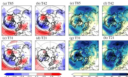
Figure 1.(a–d) Summer (JJA) 500 hPa eddy stream function (m2s−1) (shading; zonal mean removed) and zonal wind (m s−1) (contours; 10 m s−1intervals starting at 20 m s−1); (e–h) vertically integrated (total) cloudiness (%). The 500 m ice sheet topography from the LGM reconstruction is indicated by the heavy contours (interpolated to the different horizontal resolutions).
lated from the climatological monthly-mean temperature and precipitation fields, which are (bilinearly) interpolated from the atmospheric (LGM) simulations, using the above lapse rate to correct for elevation biases due to different grids and horizontal resolutions.
2.4 Atmosphere model
The atmospheric climate forcing is produced with the Com-munity Atmosphere Model version 3 (CAM3) (Collins et al., 2004; Collins et al., 2006b), using four different spectral (horizontal) resolutions: T85, T42, T31, and T21, corre-sponding to an approximate grid spacing of 1.4, 2.8, 3.8, and 5.6◦, respectively (Table 1). The model uses identical pa-rameterizations (same equations) at all horizontal resolutions (Collins et al., 2004; Collins et al., 2006b), but the climate is tuned by varying 12 parameters governing the representa-tion of clouds and precipitarepresenta-tion (convective and stratiform), biharmonic diffusion, and integration time step in order to satisfy the Courant–Friedrichs–Lewy (CFL) condition; some of the resolution-dependent parameter settings are presented in Table 1 (see Collins et al., 2004, for a complete model de-scription). Note that the model physics is represented in grid space, while the dynamics is discretized in spectral space. The effective diffusion rate is thus scale dependent and mod-ulated by (horizontal) wave number in the vorticity and di-vergence equations (Collins et al., 2004).
The planetary boundary conditions are set to reflect LGM conditions, including the orbital parameters and greenhouse gas concentrations outlined by the Paleoclimate Model-ing Intercomparison Project (PMIP) (e.g., Kageyama et al., 2017), the ice sheet reconstruction presented by Kleman et al. (2013) (raised to the height of the ICE-5G reconstruction, Peltier, 2004, to encourage ice formation in the ”correct” ar-eas in SICOPOLIS), and prescribed monthly varying surface conditions (LGM surface temperature and sea-ice extent) from Otto-Bliesner et al. (2006). Motivated by the official PMIP boundary conditions (e.g., Kageyama et al., 2017), the vegetation cover in non-glaciated areas is pre-scribed as the modern distribution.
(e) T42
−
T85
(f) T31
−
T85
(g) T21
−
T85
(d) T21
(c) T31
(a) T85
(b) T42
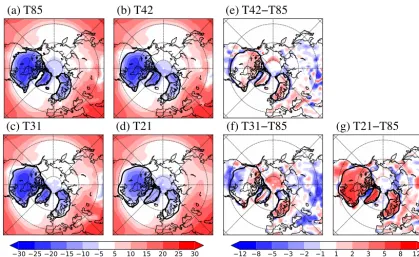
Figure 2.Summer (JJA) surface temperature (◦C) from the different resolution atmospheric climatologies. The full fields are shown in the left panels (a–d), and the difference with respect to the T85 case is shown on the right (e–g). The 500 m ice sheet topography from the LGM reconstruction is indicated by the heavy contours (interpolated to the different horizontal resolutions).
sea-surface conditions that help dampen atmospheric inter-annual variability. A longer sampling rate may alter details in the climatologies, but is not expected to change the first order conclusions from the study.
3 Climate forcing at different horizontal resolutions
In order to understand how the model climate responds to the horizontal resolution, we begin by comparing fields that are strongly related to model dynamics/physics, using the T85 case as a benchmark for the comparison. Figure 1a– d shows the 500 hPa eddy stream function (proportional to high- and low-pressure regions) and zonal wind in boreal summer (JJA). In agreement with previous studies (e.g., Dong and Valdes, 2000; Polvani et al., 2004; Magnusdottir and Haynes, 1999; Löfverström et al., 2016), the large scale atmospheric dynamics is well captured at the T42 and T31 resolutions – the circulation patterns have similar amplitude and spatial distribution as the T85 case – but it deteriorates substantially at the T21 resolution. A somewhat more grad-ual change is seen in the (vertically integrated) cloud cover (Fig. 1e–h), which is strongly controlled by the physics pa-rameterization. The cloud cover changes from about 50 % over the ice sheets in the T85 case, to almost 100 % in the T21 case.
Related to this discussion, Figs. 2 and 3 show the surface temperature and precipitation climatologies that are used as
forcing of the ice sheet model; the full fields are presented in the left columns (panels a–d), and the difference with respect to the T85 case are shown on the right (panels e–g). We fo-cus on the surface temperature in boreal summer as this is the primary ablation season, but the cumulative sum of precipi-tation over the year (total annual amount), as ice can form in all seasons in regions with a positive surface mass balance.
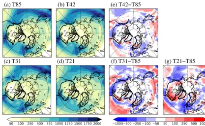
The JJA surface temperature is to first order similar in the two intermediate resolution cases (T42 and T31; Figs. 2e, f), featuring a localized warming with respect to the T85 simula-tion over the northern parts of the Laurentide ice sheet, the in-terior of the Greenland ice sheet, and most of the Eurasian ice sheet. This is partially a response to the lowering (smooth-ing) of the resolved topography on the coarser grids, but the majority of the warming is related to changes in the surface energy balance induced by the increased cloudiness (see dis-cussion in Sect. 5). The largest differences in precipitation are found in the midlatitude storm tracks that shift equator-ward relative to the T85 case, especially in the North Atlantic (Fig. 3e–g). A similar resolution-induced storm-track shift has been found in several atmospheric models (Guemas and Codron, 2011; Hourdin et al., 2012; Demory et al., 2014), and thus appears to be fairly robust and largely independent of grid type and physics parameterizations.
(e) T42
−
T85
(f) T31
−
T85
(g) T21
−
T85
(d) T21
(c) T31
(a) T85
(b) T42
Figure 3. Cumulative sum of precipitation (liquid + solid) over the year (total annual amount) (mm year−1) from the different resolution atmospheric climatologies. The full fields are shown in the left panels (a–d), and the difference with respect to the T85 case is shown on the right (e–g). The 500 m ice sheet topography from the LGM reconstruction is indicated by the heavy contours (interpolated to the different horizontal resolutions).
the lower mean-height of the resolved topography (smooth-ing from the interpolation process), but also from a general degradation of the model climate and an enhanced down-welling of longwave radiation due to the increased cloudi-ness (Fig. 1; see further discussion in Sect. 5). The midlati-tude precipitation field is also considerably altered with re-spect to the T85 case, with substantially lower precipitation in the eastern parts of the midlatitude storm tracks and thus over the southwestern parts of the ice sheets (Fig. 3). Note that this is presumably a response to the model’s inability to resolve planetary waves (and hence individual cyclones) at coarse horizontal resolutions (Fig. 1; see also Polvani et al., 2004; Magnusdottir and Haynes, 1999; Guemas and Codron, 2011; Hourdin et al., 2012; Löfverström et al., 2016).
4 Ice sheet model results
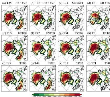
The left column in Fig. 4 shows the equilibrium ice sheet extent when using the default SMB parameterization in SICOPOLIS (SICOdef). The ice sheets forming under the high resolution atmospheric climatology (T85; Fig. 4a) are in close resemblance with the target extent (indicated by solid contours; Kleman et al., 2013), with only slightly too much ice extending in western Canada and along the Siberian Arc-tic coast.
The ice sheets forced by the intermediate resolution clima-tologies (T42 and T31; Fig.4b, c) adequately reproduce the North American ice sheet, but they fail to build the Eurasian counterpart in agreement with the reconstruction. This one-sided mismatch can be understood from the atmospheric cli-matologies described in Sect. 3. The warm summer temper-ature over the southwestern parts of the Eurasian ice sheet (Fig. 2e, f) is the main reason why ice is not forming in this region. Note that although there is a relatively small reduc-tion of precipitareduc-tion with respect to the T85 case (the inte-rior of Scandinavia is actually showing larger values than the T85 case), the warm surface temperatures are by far the most pronounced feature over the Eurasian Ice Sheet (cf. Figs. 2 and 3; see discussion in Sect. 5). These results are in broad agreement with Abe-Ouchi et al. (2013), who showed that the Eurasian ice sheet is more sensitive to temperature changes than its North American counterpart. The relatively small temperature change over the Eurasian ice sheet is thus strong enough to influence the ice sheet expansion there. The warm signal in northwestern North America (Fig. 2e, f) is located in a relatively cold region with a short ablation season, and therefore has a comparatively smaller influence on the local ice sheet evolution.
(c) T31
(a) T85
(b) T42
(d) T21
(e) T85
(i) T85
SICOdef
FST09
TP02
SICOdef
(f) T42
(j) T42
FST09
TP02
SICOdef
(g) T31
(k) T31
FST09
TP02
SICOdef
(h) T21
(l) T21
FST09
TP02
Figure 4.Equilibrium ice thickness (m) when using different ablation parameterizations in the surface mass balance scheme: (a–d) default method in SICOPOLIS; (e–h) method by Fausto et al. (2009b); and (i–l) method by Tarasov and Peltier (2002), using the atmospheric climatologies from the (a, e, i) T85; (b, f, j) T42; (c, g, k) T31; and (d, h, l) T21 resolution simulations, respectively. The 500 m ice sheet topography from the LGM reconstruction is indicated by the heavy contours (interpolated to the different horizontal resolutions).
ice sheet and instead forms two distinct ice sheets – a smaller eastern and a larger western dome – separated by a wide gap in the region around Hudson Bay. This response bears some structural similarity to the low-resolution model re-sults shown in Beghin et al. (2014) and Charbit et al. (2013), and also the pre-LGM ice sheets in Calov et al. (2005), and Bonelli et al. (2009). In a similar fashion to the T42 and T31 cases, the T21 climate forcing is too warm (and presumably too dry) over the southwestern parts of the Eurasian ice sheet area to reproduce the LGM ice sheet reconstruction.
The sensitivity experiments with different SMB parame-terizations in SICOPOLIS are presented in Fig. 4e–l. The middle row (panels e, f, g, h) uses the FST09 ablation model, and the bottom row (panels i, j, k, l) the ablation model de-scribed in TP02. Both these alternative SMB parameteriza-tions help improve the Eurasian ice extent in the T42 case (Fig. 4f, j), though at the price of a fairly substantial ice
buildup in northern Siberia and Beringia (particularly pro-nounced in Fig. 4f), which are areas that were largely ice free at the LGM (Svendsen et al., 2004; Kleman et al., 2013; Löfverström and Liakka, 2016). A broadly similar buildup in these regions is also seen in the T85 case when using these SMB parameterizations.
These alternative SMB parameterizations do not improve the ice sheet simulations in Eurasia when using the lower resolution climatologies (T31 and T21; Fig. 4g, h, k, l), but they help the formation of a continent-wide Laurentide ice sheet in the T21 case (Fig. 4k, l).
5 Discussion and conclusions
adopting a simplified modeling approach we can effectively isolate the resolution dependence of the atmospheric model, and by prescribing LGM boundary conditions (sea-surface conditions and continental ice sheets), the ice formation is primed to occur in the ”correct” areas in the subsequent ice sheet model experiments. This methodology appears to work well when using the high resolution atmospheric climatol-ogy (T85; see also Liakka et al., 2016), but is less successful when using the climatologies from the lower resolution sim-ulations (T42, T31, and T21; Fig. 4). The analysis shows that both the simulated surface temperature (Fig. 2) and precipita-tion (Fig. 3) fields are changing in ways that hinder ice from forming in the ”desired” areas at the lower resolutions. The precipitation changes are, however, found to be secondary, hence we devote the first part of this discussion to exploring the origin of the warmer surface temperatures.
There are two primarily explanations for why surface tem-peratures increase at lower horizontal resolutions: (i) lapse-rate effects due to differences in resolved topography; and (ii) changes in the simulated climate that are conducive for warm surface temperatures over the LGM ice sheets. We dis-cuss these processes in the next two paragraphs:
i. Moving to a coarser horizontal resolution typically re-sults in a lapse-rate induced surface warming, as the resolved topography is both lower and smoother as a result of the increased grid spacing. In this study we employed the modern global-average lapse rate of 6.5◦C km−1for vertical interpolation/extrapolation. This is about 1 to 2◦C km−1 higher than observations over the Greenland ice sheet in boreal summer (Fig. S2; Fausto et al., 2009a), but is motivated by the gener-ally drier conditions in glacial climates that shift the lapse rate towards higher values (Clausius–Clapeyron scaling; LGM simulations typically feature a global an-nual cooling of 4 to 6◦C relative to pre-industrial; e.g., Braconnot et al., 2007) – Loomis et al. (2017) showed that the tropical atmospheric lapse rate may have in-creased from about 5.8◦C km−1in the modern climate, to 6.7◦C km−1at the LGM. The elevation difference in the interior of the Laurentide ice sheet is around 200 m between the T85 and T21 cases (Fig. S1), hence the lapse-rate effect only accounts for 5–10 % of the local warming signal in Fig. 2. The lapse-rate effect is how-ever more important on the ice sheet edges and in Eura-sia (accounting for 30 to 50 % of the warming signal), where the difference in topography is larger.
ii. The majority of the temperature difference in Fig. 2 is induced by changes in the atmospheric circulation. The stationary planetary waves are considerably weaker in the T21 case (Fig. 1), resulting in reduced cold-air ad-vection over the Laurentide ice sheet (Fig. S3). The total cloudiness is simultaneously significantly higher (Fig. 1). While clouds help regulate the amount of downwelling shortwave radiation at the surface, upper
level ice-clouds increase the re-emission of longwave radiation back to the surface. Changes in cloudiness are found to increase the surface radiative heating effect (SWnet+ LWdown) by 10 to 30 W m−2over the LGM ice
sheets (Fig. S4).
As a result, while the T42 and T31 cases struggle to build ice in Eurasia, the T21 experiment also fails to build the continent-wide Laurentide ice sheet in North America (when using the default SMB parameterization; SICOdef). Instead it builds two spatially disconnected ice sheets, with a larger dome on the western side of the continent (Fig. 4d). Several coupled climate–ice sheet experiments with a low-resolution atmospheric model have shown qualitatively similar results, for example Calov et al. (2005), Charbit et al. (2013) and Beghin et al. (2014). The common denominator for these studies is that they all used CLIMBER-2 to produce the at-mospheric forcing fields. We stress that it is not our intention to single out this particular model, but it appears to suffer from similar deficiencies as our T21 case and may therefore help us understand some of these results. In the aforemen-tioned papers the ice sheet tends to be limited to the west-ern/northwestern side of the North American continent (e.g., Charbit et al., 2013; Beghin et al., 2014), little or no ice is es-tablished in western Eurasia (e.g., Calov et al., 2005; Char-bit et al., 2013; Beghin et al., 2014), and attempts to rem-edy these shortcomings typically result in substantial ice for-mation in Siberia and Alaska (see Charbit et al., 2013, who tested the sensitivity of the same PDD-based SMB parame-terizations as were used in this study). These results appear to be largely independent of both the choice of ice sheet model (the above studies used SICOPOLIS and GRISLI), and the complexity of the SMB parameterization (Charbit et al., 2013; Bauer and Ganopolski, 2017). Although it is not completely fair to compare CLIMBER-2 to a low resolu-tion version of CAM3 (the complexity and general purpose of these models are extremely different), it is possible that these similarities demonstrate a fundamental problem with low-resolution climate models that transcends model com-plexity.
One piece of information that is rarely mentioned in the literature is that most Earth system models are tuned to re-produce the climate of the instrument era (∼1850 to present). These models are of course valuable tools for exploring other time periods as well, but it generally means that inter-model discrepancies tend to increase under more extreme forcing scenarios, for example, glacial conditions (e.g., Braconnot et al., 2007). The results presented here suggest that the model spread may be further exacerbated by differences in horizontal resolution.
been tuned to the same standard as the other resolutions. This is probably at least a partial explanation for the appar-ent degradation of the model climate, though it is possible that this manifests a more general breakdown of the numeri-cal convergence that has been identified in previous modeling studies (e.g., Polvani et al., 2004; Magnusdottir and Haynes, 1999; Dong and Valdes, 2000). Some evidence of this is seen in Fig. 1: while the model physics shows a fairly gradual change between the T85 and T21 resolutions (Fig. 1e–h) – in-cluding a generally increased cloudiness and an equatorward migration of the mid-latitude precipitation field (a similar re-sponse to horizontal resolution has been identified in studies of the modern climate; e.g., Hack et al., 2006; Guemas and Codron, 2011; Hourdin et al., 2012; Demory et al., 2014) – fields more strongly associated with the model dynamics re-tain much of their amplitude and general structure at the T31 resolution, but deteriorate significantly when going to T21. What manifests an acceptable simulation quality is subjec-tive and highly dependent on application. However, since ice sheets are sensitive to feedback loops triggered by deviations from “expected” climate conditions (both in terms of mean state and variability), coupled climate–ice sheet simulations generally require a higher simulation quality than more tra-ditional modeling experiments.
Conversely, resorting to a lower horizontal resolution can both increase the model throughput (number of simulated years per day), and reduce the simulation cost (CPU-hours per simulated year; e.g., Yeager et al., 2006). As shown in Table 1, simulating one model year on the T85 resolution requires around 21×as many numerical operations as one model year on the T31 grid, and 48× as many operations for the same integration length on the T21 grid. This encap-sulates the challenges of coupled climate–ice sheet experi-ments, as it is common to trade resolution (”accuracy”) for computational efficiency (”speed”) in order to run transient simulations over glacial timescales.
Lastly, it is possible that some of the shortcomings dis-cussed here – e.g., the lack of ice forming in western Eurasia in the T42 and T31 cases, and in east-central North Amer-ica in the T21 case – may be due to the simplified experi-ment design and selected parameter values (some evidence of this is seen in Fig. S2). However, it is important to stress that ice evolution is ultimately controlled by the quality of the atmospheric forcing data, which we can show is strongly compromised at sufficiently coarse horizontal grids. Based on these results we conclude that a lower practical resolution bound for traditional climate model experiments is likely to be somewhere around T31, and possibly somewhat higher (nominal T42 or even T85 resolution) for coupled climate– ice sheet simulations.
Data availability. Data is available upon request from the authors.
Supplement. The supplement related to this article is available online at: https://doi.org/10.5194/tc-12-1499-2018-supplement.
Competing interests. The authors declare that they have no conflict of interest.
Acknowledgements. We thank the editor Thomas Mölg, two anony-mous reviewers, and Irina Rogozhina and Raymond Sellevold for critically evaluating this manuscript. We acknowledge Bette Otto-Bliesner and Johan Kleman and their collaborators for produc-ing and makproduc-ing publicly available the CCSM3 LGM simulation and LGM ice sheet reconstruction that were used as the basis for our experiments. The AGCM simulations were performed on re-sources provided by the Swedish National Infrastructure for Com-puting (SNIC) at the National SupercomCom-puting Center (NSC) which is financially supported by Swedish Research Council (Vetenskap-srådet; VR). The ice sheet model simulations were carried out on re-sources provided by LOEWE Frankfurt Centre for Scientific Com-puting (LOEWE-CSC).
This work was financially supported by the National Science Foundation (NSF) and the US Department of Energy (DOE).
Edited by: Thomas Mölg
Reviewed by: two anonymous referees
References
Abe-Ouchi, A., Saito, F., Kawamura, K., Raymo, M. E., Okuno, J., Takahashi, K., and Blatter, H.: Insolation-driven 100,000-year glacial cycles and hysteresis of ice-sheet volume, Nature, 500, 190–193, https://doi.org/10.1038/nature12374, 2013.
Bauer, E. and Ganopolski, A.: Comparison of surface mass bal-ance of ice sheets simulated by positive-degree-day method and energy balance approach, Clim. Past, 13, 819–832, https://doi.org/10.5194/cp-13-819-2017, 2017.
Beghin, P., Charbit, S., Dumas, C., Kageyama, M., Roche, D. M., and Ritz, C.: Interdependence of the growth of the Northern Hemisphere ice sheets during the last glaciation: the role of atmospheric circulation, Clim. Past, 10, 345–358, https://doi.org/10.5194/cp-10-345-2014, 2014.
Bonelli, S., Charbit, S., Kageyama, M., Woillez, M.-N., Ram-stein, G., Dumas, C., and Quiquet, A.: Investigating the evolution of major Northern Hemisphere ice sheets during the last glacial-interglacial cycle, Clim. Past, 5, 329–345, https://doi.org/10.5194/cp-5-329-2009, 2009.
Braithwaite, R. J. and Olesen, O. B.: Calculation of glacier ablation from air temperature, West Greenland, in: Glacier fluctuation and climate change, edited by: Oerlemans, J., 219–233, Kluwer, Dor-drecht, 1989.
Calov, R. and Greve, R.: A semi-analytical solution for the posi-tive degree-day model with stochastic temperature variations, J. Glaciol., 51, 173–175, 2005.
Calov, R., Ganopolski, A., Claussen, M., Petoukhov, V., and Greve, R.: Transient simulation of the last glacial inception. Part I: glacial inception as a bifurcation in the climate system, Clim. Dynam., 24, 545–561, 2005.
Charbit, S., Ritz, C., and Ramstein, G.: Simulations of North-ern Hemisphere ice-sheet retreat:: sensitivity to physical mech-anisms involved during the Last Deglaciation, Quaternary Sci. Rev., 21, 243–265, 2002.
Charbit, S., Ritz, C., Philippon, G., Peyaud, V., and Kageyama, M.: Numerical reconstructions of the Northern Hemisphere ice sheets through the last glacial-interglacial cycle, Clim. Past, 3, 15–37, https://doi.org/10.5194/cp-3-15-2007, 2007.
Charbit, S., Dumas, C., Kageyama, M., Roche, D. M., and Ritz, C.: Influence of ablation-related processes in the build-up of sim-ulated Northern Hemisphere ice sheets during the last glacial cycle, The Cryosphere, 7, 681–698, https://doi.org/10.5194/tc-7-681-2013, 2013.
Collins, W. D., Rasch, P. J., Boville, B. A., Hack, J. J., McCaa, J. R., Williamson, D. L., Kiehl, J. T., Briegleb, B., Bitz, C., Lin, S.-J., Zhang, M., and Dai, Y.: Description of the NCAR Com-munity Atmosphere Model (CAM3), Tech. Rep. NCAR/TN464-STR, National Center for Atmospheric Research, Boulder, CO, p. 226, 2004.
Collins, W. D., Bitz, C. M., Blackmon, M. L., Bonan, G. B., Bretherton, C. S., Carton, J. A., Chang, P., Doney, S. C., Hack, J. J., Henderson, T. B., Flato, G., Marotzke, J., Abiodun, B., Braconnot, P., Chou, S. C., Collins, W. J., Cox, P., Driouech, F., Emori, S., Eyring, V., Forest, C., Gleckler, P., Guilyardi, E., Jakob, C., Kattsov, V., Reason, C., and Rummukaines, M.: The community climate system model version 3 (CCSM3), J. Cli-mate, 19, 2122–2143, 2006a.
Collins, W. D., Rasch, P. J., Boville, B. A., Hack, J. J., McCaa, J. R., Williamson, D. L., Briegleb, B., Bitz, C., Lin, S.-J., and Zhang, M.: The Formulation and Atmospheric Simulation of the Community Atmosphere Model Version 3 (CAM3), J. Climate, 19, 2144–2161, 2006b.
Demory, M.-E., Vidale, P. L., Roberts, M. J., Berrisford, P., Strachan, J., Schiemann, R., and Mizielinski, M. S.: The role of horizontal resolution in simulating drivers of the global hydrological cycle, Clim. Dynam., 42, 2201–2225, https://doi.org/10.1007/s00382-013-1924-4, 2014.
Dolan, A. M., Koenig, S. J., Hill, D. J., Haywood, A. M., and DeConto, R. M.: Pliocene Ice Sheet Modelling Intercomparison Project (PLISMIP) – experimental design, Geosci. Model Dev., 5, 963–974, https://doi.org/10.5194/gmd-5-963-2012, 2012. Dong, B. and Valdes, P. J.: Climates at the last glacial maximum:
Influence of model horizontal resolution, J. Climate, 13, 1554– 1573, 2000.
Fausto, R. S., Ahlstrom, A. P., Van As, D., Boggild, C. E., and Johnsen, S. J.: A new present-day temperature parameterization for Greenland, J. Glaciol., 55, 95–105, 2009a.
Fausto, R. S., Ahlstrøm, A. P., Van As, D., Johnsen, S. J., Langen, P. L., and Steffen, K.: Improving surface boundary conditions with focus on coupling snow densification and meltwater reten-tion in large-scale ice-sheet models of Greenland, J. Glaciol., 55, 869–878, 2009b.
Flato, G., Marotzke, J., Abiodun, B., Braconnot, P., Chou, S. C., Collins, W. J., Cox, P., Driouech, F., Emori, S., Eyring, V., For-est, C., Gleckler, P., Guilyardi, E., Jakob, C., Kattsov, V., Rea-son, C., and Rummukaines, M.: Evaluation of Climate Models, in: Climate Change 2013: The Physical Science Basis. Contribu-tion of Working Group I to the Fifth Assessment Report of the Intergovernmental Panel on Climate Change, Climate Change, 5, 741–866, 2013.
Fyke, J. G., Sacks, W. J., and Lipscomb, W. H.: A technique for generating consistent ice sheet initial conditions for coupled ice sheet/climate models, Geosci. Model Dev., 7, 1183–1195, https://doi.org/10.5194/gmd-7-1183-2014, 2014.
Ganopolski, A., Calov, R., and Claussen, M.: Simulation of the last glacial cycle with a coupled climate ice-sheet model of intermediate complexity, Clim. Past, 6, 229–244, https://doi.org/10.5194/cp-6-229-2010, 2010.
Goosse, H., Brovkin, V., Fichefet, T., Haarsma, R., Huybrechts, P., Jongma, J., Mouchet, A., Selten, F., Barriat, P.-Y., Campin, J.-M., Deleersnijder, E., Driesschaert, E., Goelzer, H., Janssens, I., Loutre, M.-F., Morales Maqueda, M. A., Opsteegh, T., Mathieu, P.-P., Munhoven, G., Pettersson, E. J., Renssen, H., Roche, D. M., Schaeffer, M., Tartinville, B., Timmermann, A., and Weber, S. L.: Description of the Earth system model of intermediate complex-ity LOVECLIM version 1.2, Geosci. Model Dev., 3, 603–633, https://doi.org/10.5194/gmd-3-603-2010, 2010.
Greve, R.: Application of a Polythermal Three-Dimensional Ice Sheet Model to the Greenland Ice Sheet: Response to Steady-State and Transient Climate Scenarios, J. Climate, 10, 901–918, 1997.
Greve, R. and Blatter, H.: Dynamics of ice sheets and glaciers, Springer Science & Business Media, 2009.
Guemas, V. and Codron, F.: Differing impacts of resolution changes in latitude and longitude on the midlatitudes in the LMDZ atmo-spheric GCM, J. Climate, 24, 5831–5849, 2011.
Hack, J. J., Caron, J. M., Danabasoglu, G., Oleson, K. W., Bitz, C., and Truesdale, J. E.: CCSM–CAM3 climate simulation sensitiv-ity to changes in horizontal resolution, J. climate, 19, 2267–2289, 2006.
Herrington, A. and Poulsen, C.: Terminating the Last Interglacial: The role of ice sheet – climate feedbacks in a GCM asyn-chronously coupled to an ice sheet model, J. Climate, 25, 1871– 1882, 2012.
Hourdin, F., Foujols, M.-A., Codron, F., Guemas, V., Dufresne, J.-L., Bony, S., Denvil, S., Guez, L., Lott, F., Ghattas, J., Bra-connot, P., Marti, O., Meurdesoif, Y., and Bopp, L.: Climate and sensitivity of the IPSL-CM5A coupled model: impact of the LMDZ atmospheric grid configuration, Clim. Dynam., on-line first: https://doi.org/10.1007/s00382-012-1411-3, 2012. Hutter, K.: Theoretical glaciology: material science of ice and the
mechanics of glaciers and ice sheets, Reidel, Dordrecht, 1983. Jackson, C.: Sensitivity of stationary wave amplitude to regional
Janssens, I. and Huybrechts, P.: The treatment of meltwater re-tention in mass-balance parameterizations of the Greenland ice sheet, Ann. Glaciol., 31, 133–140, 2000.
Kageyama, M., Albani, S., Braconnot, P., Harrison, S. P., Hopcroft, P. O., Ivanovic, R. F., Lambert, F., Marti, O., Peltier, W. R., Pe-terschmitt, J.-Y., Roche, D. M., Tarasov, L., Zhang, X., Brady, E. C., Haywood, A. M., LeGrande, A. N., Lunt, D. J., Mahowald, N. M., Mikolajewicz, U., Nisancioglu, K. H., Otto-Bliesner, B. L., Renssen, H., Tomas, R. A., Zhang, Q., Abe-Ouchi, A., Bartlein, P. J., Cao, J., Li, Q., Lohmann, G., Ohgaito, R., Shi, X., Volodin, E., Yoshida, K., Zhang, X., and Zheng, W.: The PMIP4 contri-bution to CMIP6 – Part 4: Scientific objectives and experimental design of the PMIP4-CMIP6 Last Glacial Maximum experiments and PMIP4 sensitivity experiments, Geosci. Model Dev., 10, 4035–4055, https://doi.org/10.5194/gmd-10-4035-2017, 2017. Kleman, J., Fastook, J., Ebert, K., Nilsson, J., and Caballero,
R.: Pre-LGM Northern Hemisphere ice sheet topography, Clim. Past, 9, 2365–2378, https://doi.org/10.5194/cp-9-2365-2013, 2013.
Liakka, J.: Interactions between topographically and thermally forced stationary waves: implications for ice-sheet evolution, Tellus A, 64, 11088, https://doi.org/10.3402/tellusa.v64i0.11088, 2012.
Liakka, J., Nilsson, J., and Löfverström, M.: Interactions between stationary waves and ice sheets: linear versus nonlinear atmo-spheric response, Clim. Dynam., 38, 1249–1262, 2011. Liakka, J., Löfverström, M., and Colleoni, F.: The impact of the
North American glacial topography on the evolution of the Eurasian ice sheet over the last glacial cycle, Clim. Past, 12, 1225–1241, https://doi.org/10.5194/cp-12-1225-2016, 2016. Löfverström, M. and Liakka, J.: On the limited ice intrusion in
Alaska at the LGM, Geophys. Res. Lett., 43, 11030–11038, https://doi.org/10.1002/2016GL071012, 2016.
Löfverström, M. and Lora, J. M.: Abrupt regime shifts in the North Atlantic atmospheric circulation over the last deglaciation, Geophys. Res. Lett., 44, 8047–8055, https://doi.org/10.1002/2017GL074274, 2017.
Löfverström, M., Caballero, R., Nilsson, J., and Kleman, J.: Evo-lution of the large-scale atmospheric circulation in response to changing ice sheets over the last glacial cycle, Clim. Past, 10, 1453–1471, https://doi.org/10.5194/cp-10-1453-2014, 2014. Löfverström, M., Liakka, J., and Kleman, J.: The North American
Cordillera – An impediment to growing the continent-wide Lau-rentide Ice Sheet, J. Climate, 28, 9433–9450, 2015.
Löfverström, M., Caballero, R., Nilsson, J., and Messori, G.: Sta-tionary wave reflection as a mechanism for zonalising the At-lantic winter jet at the LGM, J. Atmos. Sci., 73, 3329–3342, https://doi.org/10.1175/JAS-D-15-0295.1, 2016.
Loomis, S. E., Russell, J. M., Verschuren, D., Morrill, C., De Cort, G., Damsté, J. S. S., Olago, D., Eggermont, H., Street-Perrott, F. A., and Kelly, M. A.: The tropical lapse rate steepened dur-ing the Last Glacial Maximum, Science Adv., 3, e1600815, https://doi.org/10.1126/sciadv.1600815, 2017.
Lora, J. M., Mitchell, J. L., and Tripati, A. E.: Abrupt reorganiza-tion of North Pacific and western North American climate dur-ing the last deglaciation, Geophys. Res. Lett., 43, 11796–11804, https://doi.org/10.1002/2016GL071244, 2016.
Magnusdottir, G. and Haynes, P. H.: Reflection of planetary waves in three-dimensional tropospheric flows, J. Atmos. Sci., 56, 652– 670, 1999.
Marsiat, I.: Simulation of the Northern Hemisphere continental ice sheets over the last glacial-interglacial cycle: experiments with a latitude-longitude vertically integrated ice sheet model coupled to a zonally averaged climate model, Paleoclimates, 1, 59–98, 1994.
Nowicki, S. M. J., Payne, A., Larour, E., Seroussi, H., Goelzer, H., Lipscomb, W., Gregory, J., Abe-Ouchi, A., and Shep-herd, A.: Ice Sheet Model Intercomparison Project (ISMIP6) contribution to CMIP6, Geosci. Model Dev., 9, 4521–4545, https://doi.org/10.5194/gmd-9-4521-2016, 2016.
Otto-Bliesner, B. L., Brady, E. C., Clauzet, G., Tomas, R., Levis, S., and Kothavala, Z.: Last glacial maximum and Holocene climate in CCSM3, J. Climate, 19, 2526–2544, 2006.
Pausata, F. S. R. and Löfverström, M.: On the enigmatic similarity in Greenland δ18O between the Oldest and Younger Dryas, Geophys. Res. Lett., 42, 10470–10477, https://doi.org/10.1002/2015GL066042, 2015.
Peltier, W.: Global glacial isostasy and the surface of the ice-age Earth: The ICE-5G (VM2) model and GRACE, Annu. Rev. Earth Planet. Sci., 32, 111–149, 2004.
Petoukhov, V., Ganopolski, A., Brovkin, V., Claussen, M., Eliseev, A., Kubatzki, C., and Rahmstorf, S.: CLIMBER-2: a climate sys-tem model of intermediate complexity. Part I: model description and performance for present climate, Clim. Dynam., 16, 1–17, 2000.
Pfeffer, W. T., Meier, M. F., and Illangasekare, T. H.: Retention of Greenland runoff by refreezing: implications for projected future sea level change, J. Geophys. Res.-Oceans, 96, 22117–22124, 1991.
Polvani, L. M., Scott, R., and Thomas, S.: Numerically converged solutions of the global primitive equations for testing the dynam-ical core of atmospheric GCMs, Mon. Weather Rev., 132, 2539– 2552, 2004.
Reeh, N.: Parameterization of melt rate and surface temperature on the Greenland ice sheet, Polarforschung, 59, 113–128, 1991. Roe, G. H. and Lindzen, R. S.: The Mutual Interaction between
Continental-Scale Ice Sheets and Atmospheric Stationary Waves, J. Climate, 14, 1450–1465, 2001.
Smith, R. S., Gregory, J. M., and Osprey, A.: A description of the FAMOUS (version XDBUA) climate model and control run, Geosci. Model Dev., 1, 53–68, https://doi.org/10.5194/gmd-1-53-2008, 2008.
Svendsen, J. I., Alexanderson, H., Astakhov, V. I., Demidov, I., Dowdeswell, J. A., Funder, S., Gataullin, V., Henriksen, M., Hjort, C., Houmark-Nielsen, M., Hubberten, H., Ingolfsson, O., Jakobsson, M., Kjaer, K., Larsen, E., Lokrantz, H., Lunkka, J. P., Lyså, A., Mangerud, J., Matiouchkov, A., Murray, A., Möller, P., Niessen, F., Nikolskaya, O., Polyak, L., Saarnisto, A., Siegert, C., Siegert, M. J., Spielhagen, R. F., and Stein, R.: Late Quater-nary ice sheet history of northern Eurasia, QuaterQuater-nary Sci. Rev., 23, 1229–1271, 2004.
Tarasov, L. and Peltier, R.: Greenland glacial history and local geo-dynamic consequences, Geophys. J. Int., 150, 198–229, 2002. Van der Veen, C. J.: Fundamentals of glacier dynamics, CRC Press,
Weertman, J.: The theory of glacier sliding, J. Glaciol., 5, 287–303, 1964.
Yeager, S. G., Shields, C. A., Large, W. G., and Hack, J. J.: The low-resolution CCSM3, J. Climate, 19, 2545–2566, 2006.