Solid Earth, 10, 931–949, 2019 https://doi.org/10.5194/se-10-931-2019
© Author(s) 2019. This work is distributed under the Creative Commons Attribution 4.0 License.
ER3D: a structural and geophysical 3-D model of central
Emilia-Romagna (northern Italy) for numerical simulation
of earthquake ground motion
Peter Klin1, Giovanna Laurenzano1, Maria Adelaide Romano1, Enrico Priolo1, and Luca Martelli2 1Centro Ricerche Sismologiche (CRS), Istituto Nazionale di Oceanografia e Geofisica Sperimentale (OGS), Sgonico (TS), Italy
2Servizio Geologico Sismico e dei Suoli, Regione Emilia-Romagna, Bologna, Italy Correspondence:Peter Klin ([email protected])
Received: 3 January 2019 – Discussion started: 15 January 2019
Revised: 19 April 2019 – Accepted: 22 May 2019 – Published: 25 June 2019
Abstract. During the 2012 seismic sequence of the Emilia region (northern Italy), the earthquake ground motion in the epicentral area featured longer duration and higher velocity than those estimated by empirical-based prediction equations typically adopted in Italy. In order to explain these anoma-lies, we (1) build up a structural and geophysical 3-D digital model of the crustal sector involved in the sequence, (2) re-produce the earthquake ground motion at some seismologi-cal stations through physics-based numeriseismologi-cal simulations and (3) compare the observed recordings with the simulated ones. In this way, we investigate how the earthquake ground mo-tion in the epicentral area is influenced by local stratigraphy and geological structure buried under the Po Plain alluvium. Our study area covers approximately 5000 km2and extends from the right Po River bank to the Northern Apennine mor-phological margin in the N–S direction, and between the two chief towns of Reggio Emilia and Ferrara in the W–E di-rection, involving a crustal volume of 20 km thickness. We set up the 3-D model by using already-published geological and geophysical data, with details corresponding to a map at scale of 1:250 000. The model depicts the stratigraphic and tectonic relationships of the main geological formations, the known faults and the spatial pattern of the seismic properties. Being a digital vector structure, the 3-D model can be easily modified or refined locally for future improvements or appli-cations. We exploit high-performance computing to perform numerical simulations of the seismic wave propagation in the frequency range up to 2 Hz. In order to get rid of the finite source effects and validate the model response, we choose to reproduce the ground motion related to two moderate-size
af-tershocks of the 2012 Emilia sequence that were recorded by a large number of stations. The obtained solutions compare very well to the recordings available at about 30 stations in terms of peak ground velocity and signal duration. Snapshots of the simulated wavefield allow us to attribute the excep-tional length of the observed ground motion to surface wave overtones that are excited in the alluvial basin by the buried ridge of the Mirandola anticline. Physics-based simulations using realistic 3-D geomodels show eventually to be effec-tive for assessing the local seismic response and the seismic hazard in geologically complex areas.
1 Introduction
by the proposed numerical simulation at the predefined scale level (e.g., Fischer et al., 2015).
The present study concerns the setup of a 3-D structural model starting from geological data and the development of the corresponding geophysical model by assigning viscoelas-tic properties to each structural unit. The scope of the final 3-D geophysical model is to allow physics-based forward mod-eling of seismic wave propagation aimed at (1) explaining the ground motion peculiarities observed in past earthquakes and (2) increasing the reliability of ground motion predic-tions for possible future events (e.g., Moczo et al., 2014; Taborda and Roten, 2015; Cruz-Atienza et al., 2016). Our study focuses on the Emilia region (northern Italy), where in 2012 a relevant seismic sequence featuring the two main-shocks,MW6.1 on 20 May 2012 at 02:03:53 UTC andMW 5.9 on 29 May 2012 at 07:00:03 UTC (Rovida et al., 2016), occurred (Fig. 1).
Seismic-hazard studies are usually based on the empirical– statistical method, which makes use of ground motion pre-diction equations (GMPEs) (e.g., Barani et al., 2017a, b), with possible corrections deduced from local geological con-ditions (Grelle et al., 2016). However, occasionally the ob-served ground motion characteristics deviate considerably from the empirical–statistical predictions. Those deviations imply the presence of case-specific features in wave gener-ation or propaggener-ation (e.g., complex fault ruptures, complex geological structures, such as deep basins), which are not ad-equately considered in the derivation of the GMPE. In or-der to predict the effects of these features, we may apply numerical–deterministic methods.
An emblematic case of such deviations occurred during the 2012 Emilia seismic crisis, when unexpectedly long du-ration and large peak ground velocity (PGV) characterized the earthquake ground motion at some sites in the epicen-tral area (Priolo et al., 2012; Castro et al., 2013; Luzi et al., 2013; Barnaba et al., 2014; De Nardis et al., 2014). Those deviations have been attributed to the complexity of the geo-logical structure beneath the Po Plain, which features a very large and deep alluvial basin bounded by two largely buried thrust-and-fold systems, the Northern Apennine chain in the south and the southern Alpine ridge in the north, respectively (Boccaletti et al., 1985). In order to explain quantitatively the observed ground motion characteristics, we have built a 3-D model that describes the morphology of the buried geological structure and assigns viscoelastic properties (mass density, elastic modula and elastic quality factors) to each formation, so that it can be used for physics-based numerical modeling of the seismic wave propagation in the studied volume.
Our model is not the first 3-D model that was devel-oped for the Po Plain area. At least three research groups have carried out 3-D numerical computations of the earth-quake ground motion in the Po Plain so far. A first study was performed by Vuan et al. (2011), who simulated long-period (T >5 s) surface waves generated in the basin by strong (MW>6) earthquakes. They used a 3-D model
fea-turing realistic, irregular basin edges and a simplified depth-dependent velocity profile for the sedimentary filling of the basin. A more complex 3-D geological model was set up by Molinari et al. (2015) for simulating the earthquake ground motion in the long-period band (T >3 s). The simu-lated waveforms were compared only qualitatively with the recorded waveforms at some far-source stations in order to demonstrate the effectiveness of the 3-D geological model. A third model is the one developed by Paolucci et al. (2015), who simulated the near-source strong ground motion for the MW6.1 20 May 2012 earthquake in the frequency range 0.1– 1.5 Hz. The overall satisfactory agreement of their simulated waveforms with the empirical records is due to two key ele-ments: the extended source model (i.e., slip distribution and rupture propagation) and the 3-D structural model, which contains only two main geologic interfaces (i.e., the base of the Pliocene formation and that of the Quaternary deposits). In particular, the satisfactory simulation of the surface waves’ trains stems mainly from the shape of the interface of the base of the Quaternary deposits. We have to mention also Turrini et al. (2014), who defined the whole structure of the Po basin from its deep roots, at the Moho level, through an exhaustive analysis of all the existing structural–geological and geophysical studies. They summarize the current knowl-edge of the Po Basin structural geology into a digital, editable model that can be used to improve the geodynamic interpre-tation of the area. However, their model does not contain any geophysical parameterization, nor does it reach the level of detail that is required in our study.
P. Klin et al.: Structural and geophysical 3-D model of central Emilia-Romagna 933
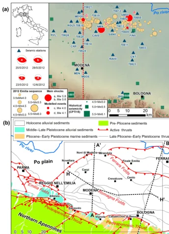
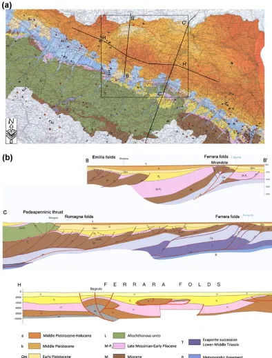
Figure 1. (a) Study area with historical seismicity (CPT15; Rovida et al., 2016), 2012 Emilia sequence epicenters (M≥3.5), tempo-rary/permanent seismological stations and trace of vertical section of Fig. 11.(b)Geological sketch of the study area, with traces of the three deep geological sections represented in Fig. 2.
for further improvements when new data will be available. In this first version, denoted ER3D, the model is based on the elaboration of a digital terrain model, a seismotectonic map and three deep geological sections crossing the study area, as well as the isobaths of two interfaces between some rele-vant geological formations. As discussed in Sect. 3.2, the de-tail level included in this model is consistent with numerical computations of the ground motion in the frequency range up
to 2 Hz and therefore comparable to the frequency range of the computations performed by Paolucci et al. (2015).
codes used in the scientific community for the 3-D simulation of the earthquake ground motion in alluvial basins, as has emerged during recent verification exercises (Maufroy et al., 2015; Chaljub et al., 2015). The validation of the constructed 3-D geological model consisted in a comparison in terms of PGV and duration, between the numerical predictions and the empirical recordings of two 2012 events at the several stations that were deployed in the area during the seismic sequence (Fig. 1). In order to put in evidence on the peculiar-ities of the ground motion that are due only to propagation effects, we considered two weak events (MW 4.0 and 4.1) that can be modeled using a point source, and not the main-shocks, which would require a finite source model. The com-putations were run using the HPC resources of the CINECA consortium in Bologna.
2 The structural and geophysical 3-D model of central Emilia
The fundamental step for physics-based numerical prediction of the earthquake ground motion consists in the setup of a 3-D model of the geological structure. In order to set up a reliable geological model, we need a sound geological in-terpretation of well-constrained geophysical data. Thanks to oil exploration and research widely undertaken since 1960, a comprehensive synthesis of the structural features of the Po Plain subsurface was possible in the past decades (e.g., Pieri and Groppi, 1981; Fantoni and Franciosi, 2010; Boccaletti et al., 2011; Martelli et al., 2017). In the following, we give an overview of the known geological features of the study area and describe how we synthetized these data in a digital 3-D structural model. Finally, we discuss how we assigned the physical properties to each geological formation for char-acterizing the 3-D model also from a geophysical point of view.
2.1 Geological and seismotectonic setting of the study area
The study area is in the Emilia-Romagna region (northern Italy), and specifically it occupies the sector of the Po Plain between Reggio Emilia (west) and Ferrara (east), as shown in Fig. 1. The Po Plain is a foredeep–foreland zone inter-posed between two chains with opposite vergence: Northern Apennines to the south and Southern Alps to the north. Ter-rigenous sediments originating from the erosion of the two growing chains accumulated in the basin (Dondi et al., 1982): first those of alpine origin (Miocene–Quaternary), then those of Apennine provenance (Pliocene–Quaternary). From the Middle Pleistocene, the sedimentation is mainly continen-tal and results from the depositional activity of the Po River and its tributaries. The substrate of the terrigenous sediments is made up by a carbonatic succession of mainly Mesozoic age, whose top consists of marly sediments of Paleogene
age. This carbonate succession is separated from the meta-morphic basement by a thick evaporite succession of Trias-sic age (Fig. 2). From the tectonic point of view, the area is affected by numerous compressive structures, with north-ern vergence (Fig. 1). The southnorth-ern zone, coinciding with the Apennine hills between the Albinea, Sassuolo, Vignola and Casalecchio di Reno municipalities, is characterized by the reverse faults of the Pedeapenninic thrust (Boccaletti et al., 1985), which is responsible for the morphological transition between the Northern Apennines and the Po Plain. Subsoil investigations for oil exploration (Pieri and Groppi, 1981) showed that the Apennine outer front does not coincide with the Apennine–Po Plain morphological margin and that in the Po Plain subsoil many blind faults and folds are present. Actually, the Apennine outer front is located in the sub-soil around the present course of the Po River, coinciding with the reverse faults of the Ferrara folds overthrusting the Lombardy–Veneto monocline (Fig. 1). The main detachment and overlap levels of thrusts are the Triassic evaporites, em-bedded between the underlying metamorphic basement and the overlying succession made of Late Triassic–Oligocene carbonates, Oligo-Miocene marls and more recent terrige-nous sediments (geological sections in Fig. 2). The south-ernmost buried structures, characterizing the subsoil of the plain between Reggio Emilia, Modena and Bologna, are the eastern termination of the Emilia folds and the western termi-nation of Romagna folds. The northernmost structures are in the subsoil between Novellara, Mirandola and Finale Emilia, where they constitute the western arc of the Ferrara folds (Fig. 1), giving rise to a very pronounced ridge, whose top is very close to the surface between Novi di Modena and Mi-randola (Laurenzano et al., 2017). A large part of the interest area, in particular the central zone between Modena, Carpi and Cento, comprised between the Pedeapenninic thrust and the Ferrara folds, corresponds to a very deep syncline: the thickness of the Plio-Quaternary sediments between Modena and Crevalcore exceeds 8500 m (Pieri and Groppi, 1981).
The relationships between tectonic structures, sedimentary bodies and the surface morphology indicate that Pedeapen-ninic thrust and Ferrara folds were active also in recent times, as demonstrated by the Quaternary deposits which are de-formed and uplifted. Conversely, the Emilia and Romagna folds were active mainly in the Pliocene, being the Quater-nary deposits not deformed by these structures but included in the syncline between the Pedeapenninic thrust and the Fer-rara folds (Pieri and Groppi, 1981; Burrato et al., 2003; Boc-caletti et al., 2004, 2011; Martelli et al., 2017).
P. Klin et al.: Structural and geophysical 3-D model of central Emilia-Romagna 935
these structures are included in the database of the seismo-genic structures capable of generating strong earthquakes (DISS Working Group, 2018). The instrumental data indicate that in this area the biggest part of earthquakes has a com-pressional source mechanism (Pondrelli et al., 2006), and that the hypocentral depth (http://cnt.rm.ingv.it, last access: 27 May 2019) in the northern zone (Ferrara folds) is con-centrated in the first 15 km, while in the Apennine–Po Plain margin greater depths (15–35 km) are common.
2.2 Integration of geological data in the 3-D digital model
Geological 3-D modeling consists in the representation of a solid Earth sector by using surface and subsurface data in a computer-aided process (Mallet, 2002), which allows to shape and to visualize the current knowledge and/or to up-date it with new data. Numerous methodologies were imple-mented in several packages dedicated to the geological 3-D modeling. The package we adopt for the present work is Geo-Modeller (Guillen et al., 2004; Calcagno et al., 2006, 2008), a commercial software originally developed by the French Bureau de Recherches Géologiques et Minières (BRGM) and more recently by the Intrepid Geophysics (http://www. geomodeller.com, last access: 27 May 2019). GeoModeller is a software tool for the integration of different geometri-cal, geological and geophysical data in a geometrically co-herent 3-D geological model. The procedure is based on the potential-field interpolation (Lajaunie et al., 1997) and is par-ticularly well suited for when the available geological data consist only in some geological maps, sparse cross-sections or boreholes. The method requires as input the location of the geology interfaces and orientation data at some points. The theory behind the method describes the 3-D geologic surfaces as isopotential surfaces of a scalar potential field, with orientation vectors playing the role of the field’s gra-dient. The stratigraphic pile is defined by the chronological order of the strata and the relationships between the forma-tions in terms of either “onlap” or “erode”. The complex geology is described by different domains, each character-ized by a geological series, separated by stratigraphic or tec-tonic discontinuities. For each domain, the geology is mod-eled by a set of subparallel, smoothly curving surfaces using the potential-field functions. Co-kriging is used to obtain a solution that honors the input data (McInerney et al., 2005). Faults are taken into account as discontinuous drift functions into the co-kriging equations (Chilès et al., 2004). Refer to Calcagno et al. (2008) for a more comprehensive description of the methods implemented in GeoModeller.
To build the 3-D geological model of central Emilia, we considered a crustal volume with 70 km×70 km area and depth of 20 km, in order to include most of the 2012 seis-mic sequence hypocenters, associated with the deepest seg-ments of the active thrusts. We defined the stratigraphic pile according to the one reported on the seismotectonic map of
the Emilia-Romagna region (Boccaletti et al., 2004; Martelli et al., 2017). We imported the following data into GeoMod-eller:
– a high-resolution digital terrain model at a grid size of 10 m, provided by the Regione Emilia-Romagna Tech-nical Office (DTM lidar; Ministero dell’Ambiente e della Tutela del Territorio e del Mare) as raster image; – an excerpt of the seismotectonic map of the
Emilia-Romagna region at a scale of 1:250 000 (Boccaletti et al., 2004), which reports the main geological units outcropping in the area, as well as the active (and po-tentially active) tectonic structures;
– two deep geological sections with a scale of 1:250 000 (Boccaletti et al., 2004), constrained by borehole data and derived by interpreting reflection seismic profiles acquired in the area, which cross the study area in the NNE–SSW direction, transversally to the Apennine chain axis (traces A–A’ and B–B’ in Figs. 1 and 2); – a deep geological section with a scale of 1:250 000
(Boccaletti et al., 2004), which crosses the study area in the WNW–ESE and W–E directions, longitudinally to the Apennine chain axis (trace H–H’ in Figs. 1 and 2); – isobaths of the plain deposits’ bottom (Formation A
with age 0.45 Myr in Fig. 3a) (Martelli et al., 2017). – isobaths of the Pliocene sediments’ bottom (Formation
MP with age 6.3 Myr in Fig. 3b) (CNR, 1992)
The geological cross-sections of Boccaletti et al. (2004) and Boccaletti et al. (2011) are based on more recent seismic pro-files than those used by Pieri and Groppi (1981) and take into account also stratigraphic data derived from Di Dio (1998), for the definition of the superficial part (down to a depth of approximately 300–400 m).
P. Klin et al.: Structural and geophysical 3-D model of central Emilia-Romagna 937
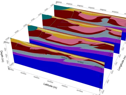
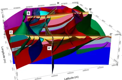
Figs. 4, 5 and 6. Two different views of the model sampled on the three input geological cross-sections are shown in Fig. 4. Figure 5 shows four parallel equally spaced north–south 2-D vertical sections across the investigated volume, while Fig. 6 evidences the surfaces corresponding to the fault system. A complete view of the 3-D model is available in the pdf file with 3-D content that is provided as the Supplement to this article. In order to use the model for numerical simulations, we exported it into voxet format by sampling the geological formation volumes with a regular 3-D grid.
2.3 Physical properties of geological formations
In order to perform the physics-based numerical simulations of the seismic wave propagation, we have to assign the val-ues of the physical properties to each 3-D geological vol-ume. Considering valid the assumption of an isotropic and viscoelastic medium, we assigned to each formation the val-ues of the following parameters:
– the velocities VP andVS of the compressional and the shear seismic wave, respectively;
– the mass densityρ;
– the elastic quality factorsQKandQµfor bulk and shear deformations, respectively.
We assumed that each geological formation belonging to the stratigraphic pile of Fig. 4 is characterized by different values of the abovementioned parameters. In order to simplify the assignment of the physical properties values to each forma-tion, we decided to characterize each unit only byVP and to evaluate from the latter the other four properties using some well-established empirical relations.
Considering the velocities expressed in km s−1, we adopted the following relation:
VS=0.7858−1.2344VP+0.7949VP2−0.1238VP3+0.0054V 4 P,
(1) which was found by Brocher (2005) from a large number of measurements made in a variety of lithologies including Quaternary alluvium and Miocene sedimentary rocks, which constitute a fundamental part of our model. We also adopted the well-established relation,
ρ=1.74VP1/4, (2)
found by Gardner et al. (1974) for the mass density ρ in g cm−3andVP in km s−1. The intrinsic attenuation is de-scribed with the shear quality factor, which is evaluated from VSexpressed in km s−1with the widely used rule of thumb (e.g., Paolucci et al., 2015):
Qµ=100VS, (3)
Figure 4.Model plotted on the three sections:(a)a southwest view,
P. Klin et al.: Structural and geophysical 3-D model of central Emilia-Romagna 939
Figure 5.3-D model: four equally spaced north–south 2-D vertical sections across the investigated volume. Stratigraphic pile as in Fig. 4c.
and with the bulk quality factor, whose value is set as
QK=3.5Qµ, (4)
in accordance with the theory exposed by Morozov (2015). We assumed that the value ofVP assigned to each geolog-ical formation might depend on the depth through a linear gradient:
VP(z)=VP(0)+∂zVPz. (5)
The values of the coefficientsVP(0)and∂zVP for each for-mation are given in Table 1. From Table 1, it appears that in most formations a constant value forVPis assumed. TheVP value in Formation A has been set to 1.5 km s−1, which cor-responds to the velocity of the compressional seismic waves in water saturated soils. The values in the deeper formations were chosen in accordance withVPvalues of the geological formations in the Po Valley basin published by Montone and Mariucci (2015).
We tested the validity of Eq. (1) by analyzing the consis-tency of the predictedVSwith some measures ofVSresulting from geophysical surveys performed in the Po Plain. Accord-ing to Eq. (1), the valueVP=1.5 km s−1assigned to the up-permost formation (Formation A) (Table 1) – having a thick-ness of the order of 100 m on most of the area – turns out
Figure 6.The fault system included in the 3-D model (east view) superimposed on the three cross-sections: B–B’, C–C’ and H–H’. Strati-graphic pile as in Fig. 4c.
Table 1.Physical quantities assigned to each geological formation.VS,ρ,QµandQKare evaluated fromVPaccording to Eqs. (1)–(4).
Formation Description VP(0)(km s−1) ∂zVP(s−1) VS(km s−1) ρ(g cm−3) Qµ QK
A Alluvial deposits up to 0.45 Myr 1.5 0 0.34 1.93 34 119
B Middle Pleistocene sands 1.5 0.5 0.34–0.61 1.93–2.07 34–61 119–213 Qm Lower Pleistocene sands 1.6 0.5 0.38–1.17 1.96–2.23 38–117 133–410 P Upper–Middle Pliocene deposits 2.6 0.1 1.08–1.48 2.21–2.3 108–148 379–519
MP Lower Pleistocene/Messinian marine 3.3 0 1.68 2.35 168 588
deposits
M Miocene flysch 3.4 0 1.77 2.36 177 620
L Allochthonous Ligurides 3.5 0 1.85 2.38 185 648
Ca Cenozoic and Mesozoic carbonates 5.5 0 3.30 2.66 330 1155
T Trias evaporites 6.0 0 3.55 2.72 355 1242
Bas Crystalline basement 6.2 0 3.64 2.75 364 1274
3 Computation of seismic waves
The computation of seismic wave propagation in alluvial basins at frequencies of engineering interest represents a de-manding task. The geometrical complexity requires the adop-tion of numerical computaadop-tional methods for the soluadop-tion of the viscoelastodynamic equation, which governs the ground motion during an earthquake. The wide range of wave ve-locities involved in realistic simulations imposes a fine sam-pling of the spatial and temporal domains. The computational cost of typical applications dictates the usage of parallel al-gorithms suitable for exploiting HPC resources.
3.1 The FPSM3D code
P. Klin et al.: Structural and geophysical 3-D model of central Emilia-Romagna 941
optimal accuracy of the global spectral differential operators and the simplicity of the spatial discretization with a struc-tured rectangular grid. According to the Nyquist’s sampling theorem, FPSM works with a relatively coarse spatial sam-pling (Fornberg, 1987), which represents a valuable advan-tage when solving 3-D problems. The FPSM3D code per-forms the time integration by means of the second-order ex-plicit finite-difference (FD) scheme and adopts the convo-lutional perfectly matching layer (C-PML) approach (Ko-matitsch and Martin, 2007) to prevent the effects of the spa-tial domain boundaries on the computed wavefield. The ef-fects of the staircase approximation of the material interfaces in the regular grid are avoided using the volume harmonic av-eraging of the elastic moduli and volume arithmetic averag-ing of the mass density, as proposed by Moczo et al. (2002). The adequateness of the FPSM3D code in this kind of appli-cations is demonstrated in the works by Chaljub et al. (2015) and Maufroy et al. (2015), aimed to estimate the accuracy of a number of numerical methods currently used for physics-based predictions of earthquake ground motion in 3-D mod-els of sedimentary basins.
3.2 Setup for the computations
A critical step in the setup for the numerical simulations con-sists in the choice of the frequency range. In order to repro-duce accurately the wave propagation at high frequencies, it requires a fine spatial and temporal sampling and there-fore a larger computational effort. On the other hand, the simulation of wavelengths much shorter than the dimensions of the heterogeneities in the model would be out of scope. We have chosen the maximum frequency (fmax) according to the detail of the 3-D geological model. The most super-ficial structural unit (i.e., Formation A) presents a variable thicknessH >50 m on a large part of the studied area and in particular at all the station locations. Considering that the average shear wave velocity assigned to this unit is about VS=0.33 km s−1, the fundamental resonance frequency (f0) of the upper layer results below 1.65 Hz, if we apply the known relationf0=VS/4H. In order to model the effects of the upper layer on the wavefield, we have to setfmax> f0. On the other hand, the lack of detail in the shallower part makes the model unsuitable for realistic computations at fre-quencies much higher thanf0; thus, we setfmax=2 Hz.
The numerical computations were performed using the spatial and temporal sampling as exposed in Table 2. The spatial domain consisted in a box with a 61.4 km wide square basis and 22 km height. The vertical sampling of the spatial grid was shrunk towards the top surface in order to sam-ple accurately the smaller wavelengths that characterize the seismic wavefield there. The flat topography of the studied area allowed us to neglect possible topographic effects. The Courant stability criterion dictated a time sampling step as short as 0.005 s, and 65 s long time series of the ground mo-tion were extracted in all the grid points at surface and on the
Table 2.Parameters defining the performed 3-D numerical simula-tions.
Max. frequency 2 Hz
Size of spatial grid 1024×1024×256 Grid cell dimensions (at surface) 60 m×60 m×10 m Grid cell dimensions (at bottom) 60 m×60 m×100 m Number of time integration steps 130 000
Time integration step 0.0005 s
Computational cost on IBM-BG/Q 50 000 core hours
two east–west and north–south vertical sections crossing the epicenter of the simulated events. We selected the length of the simulated seismograms in order to include the part of the signal that is significant for our purposes at the farthest sta-tion considered in the comparisons. The computasta-tional cost of each simulation was about 50 000 core hours on the IBM-BG/Q supercomputer at CINECA.
4 Comparisons between numerical predictions and data
In order to investigate whether the ER3D model is able to reproduce the peculiar features of the observed earthquake ground motion, we performed a comparison between the ground motion recorded by 29 seismological stations de-ployed in the study area during the 2012 seismic sequence – see Fig. 1 and Table 4 – and the numerically predicted ground motion at the same locations. The considered seismic stations belong to the Italian Strong Motion Network (IT) managed by the Civil Protection Department (DPC) and to the Italian National Seismic Network (IV) managed by the National Institute of Geophysics and Volcanology (INGV). For reference, we considered also the physics-based numer-ical predictions resulting from the simplified model PADA-NIA (Malagnini et al., 2012), which is composed of hori-zontal homogeneous layers (therefore, a 1-D model in con-trast to our 3-D). The numerical simulations regarding the PADANIA model were performed using the wavenumber in-tegration method (WIM) (Herrmann, 2013), which solves the wave equation in a horizontally layered medium. The syn-thetic seismograms contain all the phases and are accurate in both the near and far fields.
4.1 The simulated earthquake ground motion
Table 3.Parameters of the two simulated seismic events.
ID Date (DD/MM/YYYY) Time (UTC) Latitude (◦N) Longitude (◦E) Depth (km) Strike (◦) Dip (◦) Rake (◦) MW
1 12/06/2012 01:48:36 44.893 10.941 10.6 85 26 80 4.1
2 23/05/2012 21:41:18 44.847 11.250 8.9 105 33 101 4.0
Table 4.List of seismic stations.
Net code Station code Longitude (◦E) Latitude (◦N)
IT CAV0 11.0276 44.8343
IT CNT 11.2867 44.7234
IT CRP 10.8703 44.7823
IT FIN0 11.2867 44.8297
IT MDN 10.8898 44.6469
IT MOG0 10.912 44.932
IT MRN 11.0617 44.8782
IT NVL 10.7305 44.8419
IT RAV0 11.1428 44.7157
IT ROL0 10.856 44.888
IT SAN0 11.143 44.838
IT SMS0 11.235 44.934
IT ZPP 11.2044 44.5244
IV MODE 10.9492 44.6297
IV T0800 11.2479 44.8486
IV T0802 11.1816 44.875
IV T0803 11.3508 44.7668
IV T0805 11.3226 44.9187
IV T0811 11.2265 44.7838
IV T0812 11.181 44.9547
IV T0813 11.1992 44.8778
IV T0814 10.9692 44.7933
IV T0818 11.0304 44.9348
IV T0819 10.8987 44.8873
IV T0823 11.2771 44.6862
IV T0824 10.9276 44.7594
IV T0826 10.8113 44.8394
IV T0827 10.9319 44.9377
IV T0828 10.9143 44.8308
recorded waveforms are not negligible. Since the main topic of this work is the estimation of the wave propagation ef-fects on the earthquake ground motion (in particular, the in-fluence the Po Plain underground geological structure has on the wave propagation), we decided to simulate events of lower magnitude. With an upper frequency limit of 2 Hz (see Sect. 3.2), we can roughly assume that the complexities (i.e., unpredictable irregularities in the spatial extension and time evolution) in the seismic sources are negligible for earth-quakes up toMW4.0. Nevertheless, such events are strong enough to be well recorded in almost all the considered sta-tions. We therefore computed the seismic wavefield for the twoMW'4.0 events listed in Table 3 with sources located at the NE and NW ends of the studied area (events labeled c and d in Fig. 1). The hypocenters and the magnitude of these
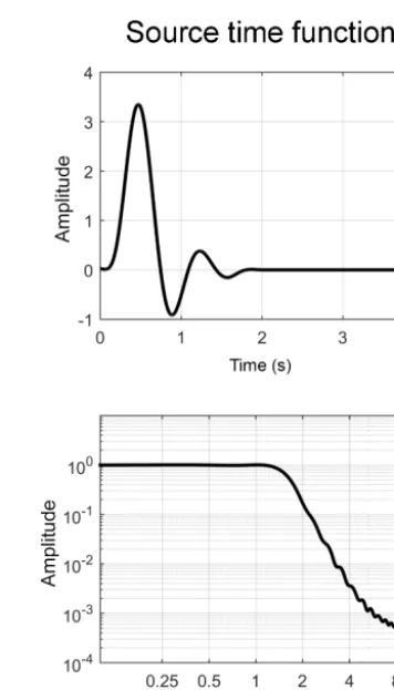
Figure 7.The time series and corresponding amplitude spectrum of the source time function used to excite the numerical simulation.
events were taken from the latest relocation study (Lavecchia et al., 2015). The generation of the wavefield was modeled as a double-couple point source with a time function corre-sponding to the low-pass minimum-phase Butterworth filter plotted in Fig. 7 and with an inverse focal mechanism, in ac-cordance to the fault plane solutions of the 2012 sequence found by Saraò and Peruzza (2012).
4.2 Comparison with the empirical earthquake ground motion
P. Klin et al.: Structural and geophysical 3-D model of central Emilia-Romagna 943
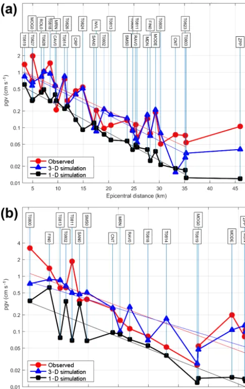
Figure 8.Observed and numerically simulated PGV (peak value of the two horizontal components) at the considered stations, plotted in function of the epicentral distance.(a)The 12 June 2012MW4.1 event.(b)The 23 MayMW4.0 event. The ordinate scale is loga-rithmic.
frequency content than the simulated ones, they were low-pass filtered using the same minimum-phase Butterworth fil-ter plotted in Fig. 7, which was used as the source time func-tion in the numerical simulafunc-tions.
We compared the simulated ground motion with the em-pirical one in terms of horizontal peak ground velocity (PGV) defined as the peak modulus of the vector sum of the two horizontal components and in the duration defined as the time interval length between 5 % and 95 % of the Arias in-tensity (Arias, 1970). The vertical component was excluded from this comparison since it was systematically lower than the horizontal ones.
In Fig. 8, we plot – separately for the two events – the log-arithm of the measured and computed PGVs at each station against the epicentral distance. We represent there also the
linear fit for the three series of data: empirical, 3-D model (ER3D) and 1-D model (PADANIA). The plot shows that, in both cases, the 3-D model numerical predictions fit the observations better, whereas the 1-D model prediction un-derestimates the observed PGV at most stations (by a fac-tor of almost 2). The high variability shown by stations at similar epicentral distance is probably due to the different source–station azimuth and focal mechanism–radiation pat-tern. As observed in Maufroy et al. (2015), the uncertainty in source characteristics may impact the numerical predictions especially at short distances. The remarkable underestima-tion of PGV for event 2 at staunderestima-tion T800, located just above the hypocenter, is therefore not too surprising and could be attributed to the combined effect of inaccurate hypocentral location, focal mechanism and near-source heterogeneities. In fact, considering that source 2 has a dip of 33◦(Table 2), T800 is near to theP-wave radiation maximum and at the margin of theS-wave lobe. Figure 10d confirms this interpre-tation: the simulated seismogram features a pronouncedP -wave amplitude in the vertical component, if compared to the S-wave one. On the other hand, in the same figure (Fig. 10d), the recorded seismogram presents a reversed picture: the rel-atively weakP wave (smaller than the simulated one) and strongSwave indicate that the actual source characteristics are different from what we assumed.
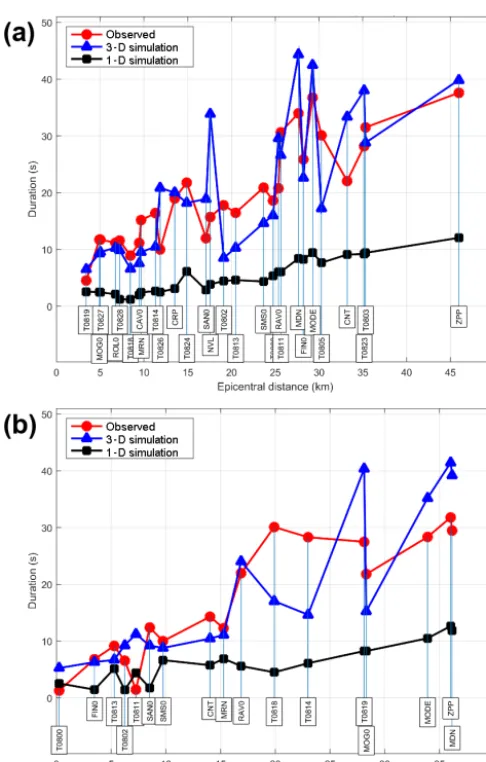
Similarly, in Fig. 9, we plot the duration of the measured and computed ground motions against the epicentral dis-tance. Again, the 3-D model numerical predictions fit better the observations than the 1-D model predictions, which un-derestimate the duration at almost all the stations. In particu-lar, it can be observed how the 3-D model is able to predict quite well the very long duration values observed at some stations located in the southern part of the model (for exam-ple, the MDN, MODE and ZPP stations for the event labeled “d” in Fig. 1). In order to analyze the reasons of the excep-tional length of the observed ground motion, we analyze, in the following section, the snapshots of the wavefield propa-gation across a north–south vertical section that encompass both the source of event d and the neighborhoods of the sta-tion MODE.
4.3 Wave propagation across a vertical profile
Figure 9. Observed and numerically simulated duration (defined as intervals between 5 % and 95 % of the Arias intensity) at the considered stations, plotted in function of the epicentral distance.
(a)The 12 June 2012MW4.1 event.(b)The 23 MayMW4.0 event.
results obtained with the 3-D model represent a significant improvement if compared to the 1-D model results.
In order to investigate the cause of the particular features of the ground motion in these stations, we can follow the modeled propagation of the seismic waves on a vertical pro-file extracted from the 3-D spatial domain (Fig. 11), whose trace on the surface is shown by the red dashed line in Fig. 1. The profile cuts the volume in the south–north direction and includes the source of the 12 June 2012 MW 4.1 event (la-beled “d” in Fig. 1) in the northern part of the section as well as the neighborhood of the T828, T824 and MODE sta-tions (represented with green triangles) in the central and southern parts. The grey shadow on the profiles represents the wave amplitude, whereas the yellow lines represent the interfaces between the structural units. For the sake of clar-ity, the structural units are labeled in Fig. 11a only. The pro-file samples three different areas of the geological structure:
the northern, central and southern parts. The northern area is characterized by the Ferrara folds (Fig. 1), where high-velocity layers (VS=1.7 km s−1) are lifted up to few tens of meters below the surface. The central area is characterized by a deep syncline with thick, low-velocity (VS<1 km s−1) superficial layers of sediments and alluvial deposits. In the southern part, we find the Emilia folds, which again reduce the thickness of the soil cover. In the first snapshot, taken after 2 s of propagation (Fig. 11a), we can see the initially concentric wavefronts propagating from the source located in the Ferrara folds. After 4 s (Fig. 11b), the wavefronts prop-agating towards south assume an almost plane shape, after having been deformed in the slower formations of the basin. We can clearly discern the compressional waves (denoted by the letterP), and the shear waves (denoted by the letterS), the latter stronger and slower, with a shorter wavelength. Af-ter 8 s (Fig. 11c), the directS has reached T828 and we can observe how at that time theSwave is reflected from the soil surface above the ridge and channeled in the dipping layers south of it. Because of the layers’ dip, the reflectedSwave hits the layers at a post-critical angle and generates a number of diffracted waves, which correspond to surface wave over-tones, if we adopt a mathematically more elegant formalism. After 16 s (Fig. 11d), the aforementioned diffracted waves can be well recognized in the profile across the wavefield and we can associate them with the strong phases following the directSarrival at the three considered stations.
For example, the strong wave train predicted at T824 be-tween 16 and 20 s of propagation (Fig. 10b) corresponds to the refracted wave on the interface between layers P and MP. The subsequent wave trains at about 23 and 28 s correspond to the refraction on the Qm-P and B-Qm interfaces, respec-tively, as it appears from the snapshot at 32 s (Fig. 10e). The refraction on these three interfaces originates also the three most evident wave trains at the end of the signal at MODE, as can be understood from Fig. 10e and f.
The lack of a stricter match between the predicted and ob-served wave trains can be ascribed to the uncertainties in the layer geometries and physical properties and does not affect the explanation we provided here for the long duration of the ground motion in the stations south of the 12 June 2012 MW4.1 epicenter.
5 Conclusions
P. Klin et al.: Structural and geophysical 3-D model of central Emilia-Romagna 945
Figure 10.Comparison between recorded (in black) and predicted (in red is the 3-D model and in blue the 1-D model) ground velocity time series and Fourier amplitude spectra in four cases.(a–c)The June 2012MW4.1 event at three stations (T0828, T0824 and MODE), southward of the epicenter: the ground motion predicted from the 3-D model results significantly more consistent with the observations than the one predicted from the 1-D model.(d)The May 2012MW4.0 event in station T0800 just above the hypocenter: the underestimation of theS-wave peak and the overestimation of theP-wave peak suggest that the actual source mechanism could be different from what we assumed (see text).
seismic crisis, characterized by unexpectedly long duration and large PGV, we developed a 3-D digital geological model of a limited area (a square with 70 km long side) of the Po Valley basin by considering already published geological and geophysical data. We applied physics-based 3-D numerical modeling to predict a posteriori the anomalous ground ve-locity duration and peak values from the developed model, finding a good correspondence. On the contrary, the predic-tion performed on the basis of a simplified model consisting of horizontal flat layers significantly underestimates these pa-rameters. From the snapshots of the numerically evaluated seismic wavefield, we could understand that the long
Figure 11.Numerically evaluated seismic wavefield for the June 2012MW4.1 event across the south–north vertical section represented in Fig. 1 (red dashed line). Green triangles: projection of the nearby station locations. Yellow star: hypocenter. Yellow lines: interfaces among structural units.(a)Snapshot taken after 2 s of propagation. Black letters: structural unit identifiers – see Table 1.(b)Snapshot taken after 4 s of propagation.P andS: wavefronts of the compressional and shear body waves, respectively.(c)Snapshot taken after 8 s of propagation.
(d)Snapshot taken after 16 s of propagation. TheSwaves dominate the scene. The dashed turquoise line denotes the ray path of the waveform reflected from the surface; the dashed cyan line denotes the total reflection on the interface between the MP andP units.(e, f)Snapshots taken after 32 and 52 s of propagation, respectively. Surface wave overtones are clearly visible in the soft soil layers in the upper part of the structure. The dashed cyan lines evidence the wave trains as well as the corresponding interfaces that originate the total reflection. The full sequence of snapshots is available as a movie file on the Open Science Framework (Klin, 2019).
Some persisting inconsistencies between the predicted and observed data can be attributed to local errors in the 3-D model as well as to errors in the assumed source parameter-ization for the simulated earthquakes. Additional data from more recent and/or still ongoing studies in the area (e.g., Mi-randola borehole by Laurenzano et al., 2017) could allow us to improve the model. The performed tests nevertheless rep-resent an encouraging step towards a deeper understanding of the seismic hazard in the Po Plain and in similar alluvial valleys worldwide.
Code availability. The digital 3-D geological model was set up with the commercial GeoModeller 3.3 software (https://www. intrepid-geophysics.com; Intrepid Geophysics, 2019). The numeri-cal simulations of seismic wave propagation were performed with HPC software developed at Istituto Nazionale di Oceanografia e di Geofisica Sperimentale (OGS) and available from the correspond-ing author upon request.
down-P. Klin et al.: Structural and geophysical 3-D model of central Emilia-Romagna 947
loaded from the Italian Accelerometric Archive – ITACA (2019, http://itaca.mi.ingv.it).
Video supplement. The snapshots of the simulated wavefield in Fig. 11 are taken from a motion picture, which is available on the Open Science Framework (https://osf.io) at the ER3D project repos-itory (https://doi.org/10.17605/OSF.IO/G7PKR, Klin, 2019).
Supplement. The supplement related to this article is available online at: https://doi.org/10.5194/se-10-931-2019-supplement.
Author contributions. LM conceived the work and selected the rel-evant geological data for the model construction; EP coordinated the project activities. GL and MAR assembled the digital 3-D geo-logical model; PK performed the numerical predictions.
Competing interests. The authors declare that they have no conflict of interest.
Acknowledgements. The present work was accomplished un-der the project “Modellazioni numeriche 3-D per il cal-colo del moto del suolo e della risposta sismica in Emilia-Romagna”, funded by Regione Emilia-Romagna. Additional sup-port was provided by the program HPC Training and Re-search for Earth Sciences (HPC-TRES) (http://www.ogs.trieste.it/ en/content/hpc-training-and-research-earth-sciences-hpc-tres, last access: 27 May 2019). The authors thank the anonymous review-ers for their helpful comments and suggestions.
Review statement. This paper was edited by Irene Bianchi and re-viewed by two anonymous referees.
References
Arias, A.: Seismic Design for Nuclear Power Plants, edited by: Hansen, R. J., Measure of earthquake intensity, Massachusetts Inst. of Tech. Press, 438–483, 1970.
Barani, S., Albarello, D., Massa, M., and Spallarossa, D.: Influence of twenty years of research on ground-motion prediction equa-tions on probabilistic seismic hazard in Italy, B. Seismol. Soc. Am., 107, 240–255, https://doi.org/10.1785/0120150276, 2017a. Barani, S., Albarello, D., Spallarossa, D., and Massa, M.: Empirical scoring of ground motion prediction equations for probabilistic seismic hazard analysis in Italy including site effects, Bull. Earth. Eng., 15, 2547–2570, https://doi.org/10.1007/s10518-016-0040-3, 2017b.
Barnaba, C., Laurenzano, G., Moratto, L., Sugan, M., Vuan, A., Pri-olo, E., Romanelli, M., and Di Bartolomeo, P.: Strong-motion observations from the OGS temporary seismic network during the 2012 Emilia sequence in northern Italy, Bull. Earth. Eng., 12, 2165–2178, https://doi.org/10.1007/s10518-014-9610-4, 2014.
Boccaletti, M., Coli, M., Eva, C., anf G. Giglia, G. F., Lazzarotto, A., Merlanti, F., Nicolich, R., Papani, G., and Postpischl, D.: Considerations on the seismotectonics of the Northern Apen-nines, Tectonophysics, 117, 7–38, 1985.
Boccaletti, M., Bonini, M., Corti, G., Gasperini, P., Martelli, L., Piccardi, L., Tanini, C., and Vannucci, G.: Seismotectonic Map of the Emilia–Romagna Region in Scale 1:250,000, With Ex-planatory Notes, CD–ROM, regione Emilia-Romagna, Servizio Geologico Sismico e dei Suoli, CNR – Istituto di Geoscienze e Georisorse Sezione di Firenze, 2004.
Boccaletti, M., Corti, G., and Martelli, L.: Recent and active tecton-ics of the external zone of the Northern Apennines (Italy), Int. J. Earth Sci., 100, 1331–1348, https://doi.org/10.1007/s00531-010-0545-y, 2011.
Brocher, T. M.: Empirical Relations between Elastic Wavespeeds and Density in the Earth’s Crust, B. Seismol. Soc. Am., 95, 2081–2092, https://doi.org/10.1785/0120050077, 2005. Burrato, P., Ciucci, F., and Valensise, G.: An inventory of the river
anomalies in the Po Plain, Northern Italy: evidence for active blind thrust faulting, Ann. Geophys., 46, 865–882, 2003. Calcagno, P.: 3D GeoModelling for a Democratic Geothermal
In-terpretation, in: Proceedings World Geothermal Congress 2015, Melbourne, Australia, 19–25 April 2015, 2015.
Calcagno, P., Courrioux, G., Guillen, A., Fitzgerald, D., and Mcin-erney, P.: How 3D implicit geometric modelling helps to un-derstand geology: The 3Dgeomodeller methodology, in: IAMG 2006 – 11th International Congress for Mathematical Geology: Quantitative Geology from Multiple Sources, 2006.
Calcagno, P., Chilès, J., Courrioux, G., and Guillen, A.: Geolog-ical modelling from field data and geologGeolog-ical knowledge. Part I. Modelling method coupling 3D potential-field interpolation and geological rules, Phys. Earth Planet. In., 171, 147–157, https://doi.org/10.1016/j.pepi.2008.06.013, 2008.
Castro, R., Pacor, F., Puglia, R., Ameri, G., Letort, J., Massa, M., and Luzi, L.: The 2012 may 20 and 29, Emilia earthquakes (Northern Italy) and the main aftershocks: S-wave attenuation, acceleration source functions and site effects, Geophys. J. Int., 195, 597–611, https://doi.org/10.1093/gji/ggt245, 2013. Chaljub, E., Maufroy, E., Moczo, P., Kristek, J., Hollender, F.,
Bard, P.-Y., Priolo, E., Klin, P., de Martin, F., Zhang, Z., Zhang, W., and Chen, X.: 3-D numerical simulations of earth-quake ground motion in sedimentary basins: testing accu-racy through stringent models, Geophys. J. Int., 201, 90–111, https://doi.org/10.1093/gji/ggu472, 2015.
Chilès, J., Aug, C., Guillen, A., and Lees, T.: Modelling the Ge-ometry of Geological Units and its Uncertainty in 3D From Structural Data: The Potential–Field Method, in: Proceedings of Orebody Modelling and Strategic Mine Planning, 313–320, AusIMM, Perth, WA, 2004.
CNR: Structural Model of Italy, 1:500,000, Quaderni La Ricerca Scientifica n. 114, CNR – Prog. Fin. Geodin. S.P. 5, 1992. Cruz-Atienza, V. M., Tago, J., Sanabria-Gómez, J. D., Chaljub, E.,
Etienne, V., Virieux, J., and Quintanar, L.: Long Duration of Ground Motion in the Paradigmatic Valley of Mexico, Scientific Reports, 6, 38807, https://doi.org/10.1038/srep38807, 2016. De Nardis, R., Filippi, L., Costa, G., Suhadolc, P., Nicoletti, M., and
Di Dio, G. (Ed.): Riserve idriche sotterranee della Regione Emilia-Romagna, Regione Emilia–Romagna – ENI Agip, Divisione Es-plorazione e Produzione, S.EL.CA., Florence, 1998 (in Italian). DISS Working Group: Database of Individual Seismogenic Sources
(DISS), Version 3.2.1: A compilation of potential sources for earthquakes larger than M 5.5 in Italy and surround-ing areas, available at: http://diss.rm.surround-ingv.it/diss/ (last access: 27 May 2019), istituto Nazionale di Geofisica e Vulcanologia, 2018.
Dondi, L., Mostardini, F., and Rizzini, A.: Evoluzione sedimenta-ria e paleogeografica nella Pianura Padana, Guide Geologiche Regionali, Soc. Geol. Ital., edited by: Cremonini, G. and Ricci Lucchi, F., 47–58, 1982 (in Italian).
Fantoni, R. and Franciosi, R.: Tectono-sedimentary setting of the Po Plain and Adriatic foreland, Rend. Fis. Acc. Lincei, 21, 197–209, https://doi.org/10.1007/s12210-010-0102-4, 2010.
Fischer, T., Naumov, D., Sattler, S., Kolditz, O., and Walther, M.: GO2OGS 1.0: a versatile workflow to integrate complex geologi-cal information with fault data into numerigeologi-cal simulation models, Geosci. Model Dev., 8, 3681–3694, https://doi.org/10.5194/gmd-8-3681-2015, 2015.
Fornberg, B.: The pseudospectral method: Comparisons with finite differences for the elastic wave equation, Geophysics, 52, 483– 501, 1987.
Gardner, G. H. F., Gardner, L. W., and Gregory, A. R.: Formation velocity and density; the diagnostic basics for stratigraphic traps, Geophysics, 39, 770–780, https://doi.org/10.1190/1.1440465, 1974.
Grelle, G., Bonito, L., Lampasi, A., Revellino, P., Guerriero, L., Sappa, G., and Guadagno, F. M.: SiSeRHMap v1.0: a simula-tor for mapped seismic response using a hybrid model, Geosci. Model Dev., 9, 1567–1596, 2016.
Guillen, A., Courrioux, G., Calcagno, P., Lane, R., Lees, T., and McInerney, P.: Constrained gravity 3D litho-inversion ap-plied to Broken Hill, ASEG Extended Abstracts, 2004, 1–6, https://doi.org/10.1071/ASEG2004ab057, 2004.
Herrmann, R.: Computer programs in seismology: An evolving tool for instruction and research, Seismol. Res. Lett., 84, 1081–1088, https://doi.org/10.1785/0220110096, 2013.
Intrepid Geophysics: https://www.intrepid-geophysics.com, last ac-cess: 27 May 2019.
ITACA: http://itaca.mi.ingv.it, last access: 27 May 2019.
Klin, P.: ER3D: Structural and geophysical 3D model of central Emilia-Romagna, public project on the Open Science Frame-work, https://doi.org/10.17605/OSF.IO/G7PKR, 2019.
Klin, P., Priolo, E., and Seriani, G.: Numerical simulation of seis-mic wave propagation in realistic 3-D geo-models with a Fourier pseudo-spectral method, Geophys. J. Int., 183, 905–922, 2010. Komatitsch, D. and Martin, R.: An unsplit convolutional perfectly
matched layer improved at grazing incidence for the seismic wave equation, Geophysics, 72, SM155–SM167, 2007. Kreiss, H.-O. and Oliger, J.: Comparison of accurate methods for
the integration of hyperbolic equations, Tellus, 24, 199–215, 1972.
Lajaunie, C., Courrioux, G., and Manuel, L.: Foliation fields and 3D cartography in geology: Principles of a method based on poten-tial interpolation, Math. Geol., 29, 571–583, 1997.
Laurenzano, G., Priolo, E., Mucciarelli, M., Martelli, L., and Romanelli, M.: Site response estimation at Mirandola by
virtual reference station, Bull. Earth. Eng., 15, 2393–2409, https://doi.org/10.1007/s10518-016-0037-y, 2017.
Lavecchia, G., de Nardis, R., Costa, G., Tiberi, L., Ferrarini, F., Cirillo, D., Brozzetti, F., and Suhadolc, P.: Was the Mi-randola thrust really involved in the Emilia 2012 seismic se-quence (northern Italy)? Implications on the likelihood of trig-gered seismicity effects, B. Geofis. Teor. Appl., 56, 461–488, https://doi.org/10.4430/bgta0162, 2015.
Luzi, L., Pacor, F., Ameri, G., Puglia, R., Burrato, P., Massa, M., Augliera, P., Franceschina, G., Lovati, S., and Castro, R.: Overview on the Strong-Motion Data Recorded during the May-June 2012 Emilia Seismic Sequence, Seismol. Res. Lett., 84, 629–644, https://doi.org/10.1785/0220120154, 2013.
Malagnini, L., Herrmann, R. B., Munafò, I., Buttinelli, M., Anselmi, M., Akinci, A., and Boschi, E.: The 2012 Fer-rara seismic sequence: Regional crustal structure, earthquake sources, and seismic hazard, Geophys. Res. Lett., 39, L19302, https://doi.org/10.1029/2012GL053214, 2012.
Mallet, J.-L. L.: Geomodeling, Oxford University Press, Inc., New York, NY, USA, 2002.
Martelli, L., Bonini, M., Calabrese, L., Corti, G., Er-colessi, G., Molinari, F. C., Piccardi, L., Pondrelli, S., and Sani, F.: Seismotectonics map of the Emilia-Romagna Region and surrounding areas, 1:250,000 scale, available at: http://ambiente.regione.emilia-
romagna.it/it/geologia/pubblicazioni/cartografia-geo-tematica/carta- sismotettonica-della-regione-emilia-romagna-e-aree-limitrofe-edizione-2016 (last access: 27 May 2019), regione Emilia-Romagna, Servizio Geologico Sismico e dei Suoli, 2017.
Maufroy, E., Chaljub, E., Hollender, F., Kristek, J., Moczo, P., Klin, P., Priolo, E., Iwaki, A., Iwata, T., Etienne, V., De Martin, F., Theodoulidis, N. P., Manakou, M., Guyonnet-Benaize, C., Piti-lakis, K., and Bard, P.-Y.: Earthquake Ground Motion in the Mygdonian Basin, Greece: The E2VP Verification and Valida-tion of 3D Numerical SimulaValida-tion up to 4 Hz, B. Seismol. Soc. Am., 105, 1398–1418, 2015.
McInerney, P., Guillen, A., Courrioux, G., Calcagno, P., and Lees, T.: Building 3D Geological Models Directly from the Data? A new approach applied to Broken Hill, Australia, in: Digital Map-ping Techniques ’05 – Workshop Proceedings, Baton Rouge, Louisiana, 2005.
Milana, G., Bordoni, P., Cara, F., Di Giulio, G., Hailemikael, S., and Rovelli, A.: 1D velocity structure of the Po River plain (Northern Italy) assessed by combining strong motion and ambient noise data, B. Earthq. Eng., 12, 2195–2209, https://doi.org/10.1007/s10518-013-9483-y, 2014.
Moczo, P., Kristek, J., Vavryˇcuk, V., Archuleta, R. J., and Halada, L.: 3D Heterogeneous Staggered-Grid Finite-Difference Model-ing of Seismic Motion with Volume Harmonic and Arithmetic Averaging of Elastic Moduli and Densities, B. Seismol. Soc. Am., 92, 3042–3066, 2002.
Moczo, P., Kristek, J., and Gális, M.: The Finite-Difference Mod-elling of Earthquake Motions. Waves and Ruptures, Cambridge University Press, Cambridge, United Kingdom, 2014.
P. Klin et al.: Structural and geophysical 3-D model of central Emilia-Romagna 949
Montone, P. and Mariucci, M. T.: P-wave Velocity, Density, and Vertical Stress Magnitude Along the Crustal Po Plain (Northern Italy) from Sonic Log Drilling Data, Pure Appl. Geophys., 172, 1547–1561, https://doi.org/10.1007/s00024-014-1022-5, 2015. Morozov, I.: On the relation between bulk and shear
seis-mic dissipation, B. Seismol. Soc. Am., 105, 3180–3188, https://doi.org/10.1785/0120150093, 2015.
Open Science Framework: https://osf.io, last access: 27 May 2019. Pacor, F., Paolucci, R., Luzi, L., Sabetta, F., Spinelli, A., Gorini, A., Nicoletti, M., Marcucci, S., Filippi, L., and Dolce, M.: Overview of the Italian strong motion database ITACA 1.0, Bull. Earth. Eng., 9, 1723–1739, 2011.
Paolucci, R., Smerzini, C., and Mazzieri, I.: Anatomy of strong ground motion: near-source records and three-dimensional physics-based numerical simulations of the Mw 6.0 2012 May 29 Po Plain earthquake, Italy, Geophys. J. Int., 203, 2001–2020, 2015.
Pieri, M. and Groppi, G.: Subsurface Geological Structures of the Po Plain, Publication 414, CNR, progetto Finalizzato Geodinam-ica, 1981.
Pondrelli, S., Salimbeni, S., Ekström, G., Morelli, A., Gasperini, P., and Vannucci, G.: The Italian CMT dataset from 1977 to the present, Phys. Earth Planet. In., 159, 286–303, https://doi.org/10.1016/j.pepi.2006.07.008, 2006.
Priolo, E., Romanelli, M., Barnaba, C., Mucciarelli, M., Lauren-zano, G., Dall’Olio, L., Abu Zeid, N., Caputo, R., Santarato, G., Vignola, L., Lizza, C., and Di Bartolomeo, P.: The Ferrara thrust earthquakes of May–June 2012: Preliminary site response anal-ysis at the sites of the OGS temporary network, Ann. Geophys., 55, 591–597, 2012.
Rovida, A., Locati, M., Camassi, R., Lolli, B., and Gasperini, P.: CPTI15, the 2015 version of the Parametric Catalogue of Ital-ian Earthquakes, https://doi.org/10.6092/INGV.IT-CPTI15, isti-tuto Nazionale di Geofisica e Vulcanologia, 2016.
Saraò, A. and Peruzza, L.: Fault-plane solutions from moment-tensor inversion and preliminary Coulomb stress analy-sis for the Emilia Plain, Ann. Geophys., 55, 647–654, https://doi.org/10.4401/ag-6134, 2012.
Taborda, R. and Roten, D.: Physics-Based Ground-Motion Simu-lation, in: Encyclopedia of Earthquake Engineering, Springer-Verlag, Berlin Heidelberg, 2015.
Turrini, C., Lacombe, O., and Roure, F.: Present-day 3D structural model of the Po Valley basin, Northern Italy, Mar. Petrol. Geol., 56, 266–289, 2014.