https://doi.org/10.5194/tc-12-1211-2018
© Author(s) 2018. This work is distributed under the Creative Commons Attribution 4.0 License.
Multi-year analysis of distributed glacier mass balance modelling
and equilibrium line altitude on King George Island,
Antarctic Peninsula
Ulrike Falk1,2, Damián A. López2,3, and Adrián Silva-Busso4,5
1Climate Lab, Institute for Geography, Bremen University, Bremen, Germany
2Center for Remote Sensing of Land Surfaces (ZFL), Bonn University, Bonn, Germany 3Institute of Geology and Mineralogy, University Cologne, Cologne, Germany
4Faculty of Exact and Natural Sciences, University Buenos Aires, Buenos Aires, Argentina 5Instituto Nacional de Agua (INA), Ezeiza, Buenos Aires, Argentina
Correspondence:Ulrike Falk (ulrike.falk@gmail.com)
Received: 12 October 2017 – Discussion started: 1 December 2017
Revised: 15 March 2018 – Accepted: 19 March 2018 – Published: 10 April 2018
Abstract. The South Shetland Islands are located at the northern tip of the Antarctic Peninsula (AP). This region was subject to strong warming trends in the atmospheric sur-face layer. Sursur-face air temperature increased about 3 K in 50 years, concurrent with retreating glacier fronts, an in-crease in melt areas, ice surface lowering and rapid break-up and disintegration of ice shelves. The positive trend in surface air temperature has currently come to a halt. Observed surface air temperature lapse rates show a high variability during winter months (standard deviations up to ±1.0 K(100 m)−1) and a distinct spatial heterogeneity re-flecting the impact of synoptic weather patterns. The in-creased mesocyclonic activity during the wintertime over the past decades in the study area results in intensified advection of warm, moist air with high temperatures and rain and leads to melt conditions on the ice cap, fixating surface air temper-atures to the melting point. Its impact on winter accumulation results in the observed negative mass balance estimates. Six years of continuous glaciological measurements on mass bal-ance stake transects as well as 5 years of climatological data time series are presented and a spatially distributed glacier energy balance melt model adapted and run based on these multi-year data sets. The glaciological surface mass balance model is generally in good agreement with observations, ex-cept for atmospheric conditions promoting snow drift by high wind speeds, turbulence-driven snow deposition and snow layer erosion by rain. No drift in the difference between sim-ulated mass balance and mass balance measurements can be
seen over the course of the 5-year model run period. The win-ter accumulation does not suffice to compensate for the high variability in summer ablation. The results are analysed to as-sess changes in meltwater input to the coastal waters, specific glacier mass balance and the equilibrium line altitude (ELA). The Fourcade Glacier catchment drains into Potter cove, has an area of 23.6 km2and is glacierized to 93.8 %. Annual dis-charge from Fourcade Glacier into Potter Cove is estimated toq¯=25±6 hm3yr−1 with the standard deviation of 8 %
annotating the high interannual variability. The average ELA calculated from our own glaciological observations on Four-cade Glacier over the time period 2010 to 2015 amounts to 260±20 m. Published studies suggest rather stable conditions of slightly negative glacier mass balance until the mid-1980s with an ELA of approx. 150 m. The calculated accumulation area ratio suggests dramatic changes in the future extent of the inland ice cap for the South Shetland Islands.
1 Introduction
but also changes in internal dynamics (Payne et al., 2004; Davis et al., 2005; Van den Broeke et al., 2006). The Antarc-tic Peninsula (AP) has been warming with a rate exceeding 0.5 K decade−1at least during the last five decades (Skvarca et al., 1999; Vaughan et al., 2003; Steig et al., 2009; Barrand et al., 2013; Falk and Sala, 2015a). This is likely caused by atmospheric and oceanic changes associated with the strato-spheric ozone depletion (Fogt and Zbacnik, 2014), strength-ening of the westerlies (Thompson and Solomon, 2002; Orr et al., 2008) and the increased presence of modified warm cir-cumpolar deep water on the continental shelf (Joughin et al., 2014). This leads to changes in sea-ice season length, extent and concentration in the neighbouring seas (Parkinson, 2002; Abram et al., 2010; Stammerjohn et al., 2012). More specifi-cally, the increase in near-surface air temperature shows sig-nificantly higher warming trends during winter months for the South Shetlands (Falk and Sala, 2015a). The east coast of the AP is mostly influenced by cold and dry air masses stem-ming from the adjacent Weddell Sea. In contrast, the west coast and the South Shetland Islands are directly exposed to the humid and relatively warm air masses from the South Pacific Ocean carried by the strong and persistent westerly winds. The interaction of the westerlies with the topography of the AP can lead to extreme foehn events on the eastern side (Cape et al., 2015).
Trends in surface air temperature in the AP have been anal-ysed and discussed in several studies obtained from meteoro-logical observations of either manned or automatic weather stations (AWSs) (Doran et al., 2002; Turner, 2004; Turner et al., 2005; Chapman and Walsh, 2007; Barrand et al., 2013; Falk and Sala, 2015a), sometimes complemented by satel-lite remote sensing data (Shuman and Stearns, 2001; Fahne-stock et al., 2002; Steig et al., 2009). These studies congru-ently show the statistical significance of the observed posi-tive trends in near-surface air temperatures of approx. 2.5 K over the last five decades along the AP and the strong cli-matic change in the AP on a regional scale. Different drivers of the observed changes have been identified for winter and summer seasons: winter sea ice concentration and mean sea level pressure anomalies are strongly connected with tropical variability, i.e. the El Niño–Southern Oscillation (Bromwich et al., 2000; Yuan, 2004; Meredith et al., 2004), whereas changes of summer month’s atmospheric circulation are driven by stratospheric ozone depletion and greenhouse gas concentrations (Thompson and Solomon, 2002; Perlwitz et al., 2008; Turner et al., 2009; Thompson et al., 2011). The seasonal variability is represented by the Southern Annular Mode (SAM) index. The SAM is a low-frequency mode of atmospheric variability that describes the north–south move-ment of the westerly wind belt around Antarctica. It shows high a positive numbers during fall–winter, associated with a contraction of the Antarctic high-pressure cell, and a vari-ability that is of the same order of magnitude as the linear trend observed over the past four decades (Falk and Sala, 2015a).
As a consequence of the observed warming, striking glaciological changes have happened along the whole length of AP’s western and eastern coasts. Studies along the AP show basal and surficial enhanced melting on ice shelves accompanied by subsequent collapse (Skvarca et al., 2004; Braun et al., 2009), widespread glacier acceleration and thin-ning (De Angelis and Skvarca, 2003), grounding line and calving front retreat (Rignot et al., 2011; Rau et al., 2004) and others. Ice shelves and glaciers of the AP region have been under a generalized retreat and disintegration trend at least during the last five decades (Rott et al., 1996; Skvarca et al., 1998; Scambos et al., 2000; Shepherd et al., 2003; Skvarca et al., 2004; Scambos et al., 2008; Braun et al., 2009). Ongo-ing atmospheric and cryospheric change are directly linked to profound changes of the adjacent ocean (Meredith and King, 2005). Marine species in the AP region show extreme sensi-tivities to environmental conditions and their changes (Smith et al., 1999; Peck et al., 2004; Ducklow et al., 2007; Clarke et al., 2007; Montes-Hugo et al., 2009; Schloss et al., 2012; Quartino et al., 2013; Abele et al., 2017). Glacial meltwater input to the coastal systems significantly changes physical and chemical properties, e.g. salinity, turbidity, light trans-mission and trace metals (Henkel et al., 2013; Sherrell et al., 2015). These studies rely on an accurate estimation of glacier melt.
Systematic glaciological field studies are very scarce on both sides of the AP and in especially there are none that try to sufficiently capture inter- and intra-annual variability. In this paper, we present a 6-year record of continuous glacio-logical observations obtained on very high temporal resolu-tion to resolve winter melt periods and properly define the start of glacial accumulation and ablation periods. The time series is analysed with regard to climatic drivers and glacial melt is estimated to provide the necessary boundary condi-tions for interdisciplinary studies on the ongoing changes in the biota and species composition of the coastal waters in the South Shetland region. The following sections will describe the meteorological and glaciological data time series, evalu-ate calibration and validation of the glaciological model, and discuss surface mass balance and simulated glacial discharge with regard to seasonal and interannual variability. Finally, results of equilibrium line altitude (ELA) and accumulation area ratio (AAR) are used to assess future glacier extent.
The main scientific objective of this paper is to investigate the impact of the concurrent climatic conditions on meltwater discharge to the coastal environments and the glacier ELA, which sets the boundary conditions for the observed envi-ronmental change.
2 Study area
Figure 1.Map of research area on King George Island (South Shetland Islands, northern Antarctic Peninsula) including the locations of our own installations and external data time series. Potter creek basins of Potter North and Potter South with drainage channels and mass balance stake locations along two transects, PG0xand PG1x(wherexis a placeholder for stake number), in the catchment area. Background: SPOT-4, 18 November 2010, © ESA TPM, 2010.
are relatively uniform and smooth, whereas the south-facing coast and slopes are rugged and steep. Around 90 % of its 1250 km2 area is covered by a polythermal ice cap and is influenced by its maritime climate. Rückamp and Blindow (2012) have surveyed a significant part of it, finding that the mean ice thickness is approx. 240 m, with a maximum value of 422 m. The maximum elevation is 720 m a.s.l.in the cen-tral ice dome, with frequent secondary maxima of about 500– 600 m a.s.l. across the island (Rückamp et al., 2011). The ice cap is divided into drainage basins according to the un-derlying geological structure (Braun and Hock, 2004). The different draining glaciers end either on land or as tidewa-ter glaciers. Most of the glacier systems on the South Shet-land IsShet-lands have shown significant retreats in recent past (Birkenmajer, 2002; Braun and Gossmann, 2002; Cook et al., 2005; Rückamp et al., 2011). The Warszawa Icefield cov-ers the southwestern part of KGI including the Potter Penin-sula. It includes two tidewater glaciers: Polar Club Glacier and Fourcade Glacier. The latter drains into Potter Cove. Our data were mainly obtained on these two glaciers or in the neighbouring areas (see map in Fig. 1). Jiahong et al. (1998) and Ferron et al. (2004) report an annual average surface air temperature of−2.4 and−2.8◦C, respectively. Falk and Sala (2015a) show a strong positive trend in surface air tempera-ture especially in the winter, whereas for the summer month
December the trend is slightly negative over the past four decades. In general, days with temperatures above freezing are rarely absent in winter and are frequent in summer. The occurrence of temperatures above the melting point all year round is well recorded by thick and multiple ice lenses even in high elevations of the ice cap. Air temperatures above the melting point are generally associated with presence of low-pressure systems and advection of warm and moist air from the mid-latitudes over the surrounding oceans often resulting in precipitation in form of rain (Parish and Bromwich, 2007).
3 Data and methods
Figure 2.AWS installed on the Fourcade Glacier with view to the Potter Cove and Three Brothers Hill. The photo was taken during winter on 30 May 2012.
3.1 Meteorological data sets
3.1.1 Meteorological measurements on Fourcade and Polar Club glaciers, Potter Peninsula, KGI
An AWS was installed in November 2010 at 62◦14009.800S and 58◦36048.700W at 196 m a.s.l., close to the approximate divide of Fourcade and Polar Club glaciers, which are both part of Warszawa Icefield. The AWS is equipped with wind anemometers and vanes (Alpine Wind Monitor); air temper-ature and relative humidity sensors (HMP155A) at 1.4 and 2.5 m above ground; and snow and ice temperature mea-surements (107 thermistor probes) installed at 10, 5 and 1 m depth in the glacier and 0.1 and 0.3 m above ground to mea-sure snow temperature during winter. The AWS included a four-component radiation sensor (NR01) for up- and down-welling long- and shortwave radiation fluxes, two narrow-field infrared temperature sensors (IR120) facing northwest and southeast at a zenith angle of 40◦ to measure surface temperatures, and a sonic ranging sensor (SR50A) installed at an initial height of 1.9 m to measure surface elevation changes. For data acquisition and storage, a CR3000 Mi-crologger with extended temperature testing was used. The meteorological sensors were installed on a 3 m tripod that was fixed to 3 m aluminum poles drilled into the ice. The AWS is shown in Figs. 2 and 3. To ensure good quality of radiation measurements, all radiation sensors were mounted at a 3 m boom extended from the tripod and fixed to addi-tional poles drilled into the ice. Levelling and adjustment of sensors were carried out according to ablation and accumu-lation. In case it was necessary outside of periods of summer field campaigns, this work was carried out by the overwin-tering scientist at Carlini Station. In particular at the end of the ablation season, the whole system needed to be lowered
Figure 3. AWS installed on the Fourcade Glacier with view to the Potter Cove and Three Brothers Hill. The photo was taken on 4 March 2012 and shows the AWS during the ablation period when pyroclastic material resurface due to melting of the winter snow layer.
with a maximum of 2 to 3 m each year due to ablation at the AWS station. Power supply was realized with solar pan-els and a battery stack. Measurement rate was set to every 5 s with an averaging interval of 10 min. During the summer field campaign January–March 2012, an additional AWS (de-noted as ZAWS) was installed in the accumulation area of the Warszawa Icefield at 62◦1205.700S and 58◦34058.400W at 424 m a.s.l.to measure wind speed and direction, air temper-ature and relative humidity, as well as downward shortwave radiation (Li190SB) for the time period of 2 weeks. All sen-sors and station equipment were purchased from Campbell Scientific, Logan, Utah. Four additional air temperature and data logger sensors (UTL, Geotest Schweiz) were distributed on the investigated glaciers (62◦1403200S, 58◦3505400W, 144 m a.s.l.; 62◦1305100S, 58◦3800500W, 65 m a.s.l.; 62◦130 5800S, 58◦3802800W, 36 m a.s.l.) to assess the spatial variabil-ity and lapse rates of surface air temperature. One UTL sen-sor was kept at 2 m height at the AWS site to ensure the con-tinuity of air temperature records during power failure of the AWS. The meteorological data time series and climatology of the Potter Peninsula are discussed in detail by Falk and Sala (2015a).
3.1.2 Meteorological observations at Carlini Station
velocity, barometric pressure and cloudiness (SMN, 2016). This time series was resampled to hourly data by linear inter-polation and smoothed by applying a moving average with a 24 h window to yield a more realistic daily course. The data set was used to investigate lapse rates between the AWS and Carlini Station in order to gap fill the time series at the AWS during power outages. Details will be discussed in the fol-lowing sections on meteorological post-processing and gap filling.
3.1.3 Long-term climate data set of meteorological observations at Bellingshausen Station
The Russian Bellingshausen Station is located on Fildes Peninsula of KGI at 62◦1105500S, 58◦5703800W at about 14 m a.s.l.at a distance of 18.5 km to the AWS. The Belling-shausen climate observations are on 6-hourly measurements of barometric pressure, surface air temperature, dew point temperature, relative humidity, total cloud and low cloud cover, surface wind direction, surface wind speed and pre-cipitation. This time series starts in October 1968 and it is available in 6-hourly resolution (Martianov and Rakusa-Suszczewski, 1989). The time period for the analysis of this paper is from November 2010 to December 2015. The data used here were taken from AARI (2016) and were down-loaded from the Russian weather data centre (http://wdc.aari. ru/datasets/). This data set was used to reconstruct the precip-itation time series at the AWS because the ultrasonic sensor to measure distance to the surface was malfunctioning after less than a year.
3.1.4 Meteorological data processing and gap filling The 5-year meteorological data time series for the AWS lo-cation on the glacier of the Potter Peninsula was screened for flawed and unrealistic values caused either by instrument malfunctioning or by environmental impacts such as hoar frost. During wintertime, power outages are more likely to occur and maintenance is often prevented by unfavourable weather conditions. Gap-filling routines were implemented and are discussed in the following.
Methods using the monthly mean diurnal cycle to fill data gaps were rejected, because (a) data gaps in wintertime are by far more frequent and also the time period of missing data longer, and (b) the diurnal variability is dominated by the seasonal course. For each sensor, the data were checked for malfunctioning or other environmental impact, but also for statistical properties according to Falk and Sala (2015a). The meteorological data set was aggregated to hourly time steps to reduce computation time during the modelling work (see Sect. 3.3).
The AWS air temperature measurements were screened for spikes (every value outside the 6-fold standard deviation of the long-term average) and air temperature readings below −40◦C were discarded. The resulting gaps (11.6 % of the
data set) were filled with records of the UTL air tempera-ture and, where not available, were extrapolated from Car-lini (CAR) Station air temperature observations based on the monthly mean adiabatic lapse rate analysis carried out by Falk and Sala (2015a).
Apart from a crossing of a synoptic frontal system, sud-den spikes to low values in the barometric pressure are usu-ally associated with problems and sudden drops in the power supply. All values below 930 hPa were thus disregarded. The 5-year average of the barometric pressure sensor computes to 967 hPa with a maximum value of 1009 hPa. Data gaps (25 % of the data set) were then filled by extrapolating the meteorological observations at Carlini Station applying the hydrostatic equation:
pAWS=pCAR·e −9.831z
RLTAWS, (1)
where the barometric pressurepCAR is the resampled time
series at Carlini Station,1zthe elevation difference,RLthe
specific gas constant andTAWSthe AWS absolute air
temper-ature in Kelvin.
The 2 m wind velocity was screened for sensor malfunc-tioning. The cleaned 5-year statistics show a linear relation-ship between the horizontal wind speeds measured at Carlini Station and the AWS on the glacier of
vAWS=1.15·vCAR−2 m s−1, R2=0.6. (2)
This relation was used to fill the gaps in the time series of the AWS wind speed observations (25 % of the data set).
The search of a similar relationship for the relative humid-ity yielded a linear regression between the time series at Car-lini Station and at the AWS with a very poor correlation co-efficient ofR2=0.3. The comparison of first-order statistics shows that
RHAWS=1.08·RHCAR±0.5. (3)
Generally, the value range of relative humidity is between 60 and 100 %. The diurnal variability is usually of the same magnitude (σRHAWS≈0.4). For this value range the error is
thus acceptable. Values for the relative humidity are gener-ally very high at the AWS site; 25 % of the complete data set of relative humidity were gap filled.
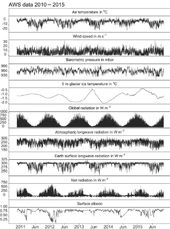
Figure 4.Meteorological time series (gap-filled) aggregated to hourly resolution at the AWS site on the Fourcade Glacier, King George Island, during the time period November 2010–November 2015.
The cloud coverage data were taken from the observations (cloud coveragec8in one-eighth of total sky area) at Carlini
Station, smoothed with a 48 h window. This window size is well adjusted not to eliminate the synoptic changes between low-pressure systems, usually associated with overcast sky, and high-pressure systems over continental Antarctica that are often accompanied with clear sky. The timescale of these changes are considered to be at least 3 days to 1 or 2 weeks. The cloudinesscis given in decimal format ofc8with a value
range between 0 and 1.
The four-component radiation sensor is prone to icing or riming due to advection of warm, moist air masses into the
region. This affects especially the upward looking sensors for long- and shortwave radiation. As criteria for detection of sensor riming, van den Broeke et al. (2004) suggest that the downward longwave radiation flux density equals the upward flux. Here, the criterion was chosen as
LW↓= |LW↑ | ±0.5 W m2, (4)
where LW↓and LW↑are the upward and downward long-wave radiation flux densities, respectively. Additionally, val-ues ofRn<−500 W m−2were discarded. The above
together with overcast skies or high cloud coverage, the ap-plied criterion was deliberately chosen as very sharp to avoid filtering real values for longwave radiation flux densities. To fill the gaps in the radiation data time series, the different up-and downward flux densities of the long- up-and shortwave com-ponents were simulated by applying basic geographic and as-tronomic equations (Campbell and Norman, 2000) using the Julian day (J), local time (t), location information (longi-tudeθand latitudeφ) in decimal-degree, absolute surface air temperature (Ta) in K, barometric pressure (Pa) in kPa,
abso-lute surface temperature (Ts) derived from ice temperatures
and upward longwave radiation measurements, cloudiness in decimal numbers (c) and the gap-filled (33 %) albedo mea-surements (α).
The optical air mass number is given for ψ <80◦ by m=Pa/(99·cosψ ), whereψ is the solar zenith angle. The
atmospheric transmittanceτ is calculated by adapting Gates (1980) to
τ =0.5+0.45(1−c) . (5)
The top-of-atmosphere (TOA) solar incidental radiation flux (SWTOA) is then computed by SWTOA=1367·cosψand the
total solar incidental radiation flux to the surface as the sum of direct (SWdirect=SWTOA·τ) and diffuse (SWdiffuse=0.4· (1−τ )·SWTOA) components by
Kdown, sim=SWTOA·τ+0.4·(1−τ )·SWTOA. (6)
The solar radiation reflected (Kup, sim) at the surface is then
calculated by multiplying the albedo to the simulated down-ward shortwave flux, i.e. the sum of diffuse and direct radia-tion flux.
The downward component of the longwave radiation bud-get at the surface is calculated using the emissivity of the atmosphere (ε=9.2·Ta2×10−6) (Monteith and Unsworth, 1990) to estimate the emissivity under cloud coverage (εac): εac=(1−0.84·c)·ε+0.84·c. (7)
Applying the Boltzmann law this gives for the longwave downward component (LW↓)
LW↓=εac·5.67×10⁻⁸·Ta4W m
−2K−4 (8)
and for the longwave upward component (LW↑) with a sur-face emissivity ofε=0.9
LW↑=0.9·5.67×10−8·Ta4W m−2K−4. (9) The statistics of the simulated radiation fluxes are then com-pared to the statistics of the measured time series, resulting in correlation coefficients generally aboveR2>0.7. The sim-ulated longwave fluxes were adjusted to the observations by fixating the mean values of the simulated to the observed val-ues. A difference in long-term average of 29 and 35.5 W m−2 was added to the simulated atmospheric longwave emittance
and simulated earth’s longwave emittance, respectively. The comparison of simulated shortwave fluxes to the long-term observations suggested a further refinement of the impact of cloud coverage on the shortwave radiation fluxes according to
Kup/down, obs=Kup/down, sim·(1−0.4·c)·1.171, (10)
with anR2=0.7. The overall comparison of the simulated (sim) and observed (obs) net radiation flux resulted in a linear regression with very good correlation:
Rn, sim=15.9+0.987·Rn, obs, R2=0.7. (11)
The root-mean-squared error amounts to 39 W m−2and the mean bias deviation to 10 W m−2. The remaining data gaps were closed using the simulated and fitted shortwave radi-ation fluxes. In summary, about 50 % of the shortwave and upward-facing radiation data needed to be gap filled with the simulated data, whereas only 25 % of the earth’s longwave radiation data were identified as missing or flawed data.
Accumulation measurements based on sonic ranging are available during November 2010 to May 2011 and March 2012 to November 2012. Outside these periods, accu-mulation was reconstructed using the readings of the Belling-shausen 6-hourly precipitation data. These were resampled to hourly data time series by linear interpolation, smoothed and normalized with the total daily sum. The mass balance stake (MBS) data at the AWS location were then used as an en-velop for the daily sums of the resulting accumulation time series. Figure 4 shows the resulting quality-controlled and gap-filled data time series of the meteorological variables. 3.2 Glaciological measurements on Fourcade Glacier,
Potter Peninsula, KGI
Table 1. Locations of the mass balance stake (MBS) at the AWS and the transects (PG0x and PG1x) on Potter Peninsula and the mass balance stake transect (PDx) on Barton Peninsula, Fourcade Glacier, on King George Island (see map in Fig. 1), during the time period November 2010 to December 2016.
MBS ID Latitude Longitude Elevation
in◦ in◦ in metres
PD07 −62.22862273 −58.71420340 46.67 PD08 −62.22600435 −58.71697602 105.91 PD09 −62.22384791 −58.71785753 144.98 PD10 −62.22116730 −58.71976533 197.37 PD11 −62.21795095 −58.71573503 235.95 PG01 −62.20148816 −58.58323580 435.74 PG02 −62.20888206 −58.58377693 385.16 PG03 −62.21753275 −58.58727917 346.35 PG04 −62.22211759 −58.59201413 294.28 PG05 −62.22706859 −58.59880010 247.94 PG06 −62.22987936 −58.60632380 223.71 PG07 −62.23522760 −58.61638383 188.65 PG08 −62.23566435 −58.62323978 159.14 PG09 −62.23580607 −58.62959815 121.04 PG11 −62.19914054 −58.58120011 465.58 PG12 −62.20550417 −58.58144177 409.88 PG13 −62.21393126 −58.58316591 357.77 PG14 −62.22063413 −58.58796499 320.17 PG15 −62.22530107 −58.59524968 263.89 PG16 −62.23067104 −58.60096266 229.45 PG17 −62.23637683 −58.62141147 167.24 PG18 −62.23711034 −58.62826182 131.35 PG19 −62.23767187 −58.63362381 96.76 AWS −62.23594584 −58.61346750 194.52
Warszawa Icefield and thereby the loss of the time series. For the measurements of stakes that were not protruding verti-cally from the ice but at an inclination caused by the high wind speeds, a geometric correction was applied to yield the correct exposition length. During the summer field cam-paigns November 2010 to March 2013, repeat measurements with differential GPS (DGPS) at static points of the MBSs yielded an average velocity for the lower transect up to eleva-tions of approx. 250 m of below 1 m a−1and up to 6.3 m a−1 for the MBSs on the upper glacier. Figure 5a shows a sam-pling at the MBS transect.
Snow density samples were taken with an aluminum snow density cutter (SnowHydro, Fairbanks, Alaska) with a de-fined volume of 0.001 m3 and a balance scale with an ac-curacy of 0.1 g (Carl Roth GmbH, Germany) calibrated at least once each summer campaign. For the snow density sam-pling, a snow pit of about 0.5 m depth was dug out and at least three sample volumes, extracted at a depth of about 0.3 m by putting the snow cutter horizontally into the pit wall, were then averaged. The snow depth was measured with a regular snow sonde used as mountaineering equipment. Around each stake about 10 measurements were taken and
then averaged. Snow densities were measured 15 Novem-ber 2010 in the glacier ablation zone and on 7 March 2011 in the glacier accumulation zone, yielding a snow density ofρs=503±16 kg m−3andρs=488±20 kg m−3,
respec-tively. On 23 January 2012, a snow pit was dug out in the accumulation zone of the Warszawa ice cap at the additional AWS (Falk and Sala, 2015a). Snow density measurements were taken every 0.2 m up to a depth of 2 m and resulted in an average value of ρs=416±47 kg m−3. The correlation
with depth was found to be not significant.
Starting in June 2012 until February 2016, regular snow density values were taken together with the MBS transect measurements. A seasonality in the snow density time se-ries is evident and presented in Fig. 6a. With rising tem-peratures during the austral summer and fall, the snow den-sity also shows rather high values up to approx. 500 kg m−3. With the onset of the winter, the precipitation changes to low-density snow, which then compacts over the course of the winter. During austral winter, the overwintering scien-tist was responsible for the glaciological measurements of the whole campaign. The snow density time series of win-ter 2015 shows a high variability and particularly low val-ues, well below any observation before. Although the values by themselves are reasonable for very cold and dry condi-tions (Patterson, 1980), the contemporary surface air temper-ature measurements do not show any behaviour that would satisfy the requirements for the very low snow density obser-vation. We therefore suspect the measurement to be affected by errors, leading to an underestimation of the snow density. This seems to have been the case during winter 2015. Thus, for the time period before June 2012 and after March 2015, mass balance and related variables were computed using the monthly averages of the period in between for snow density values. Figure 6b shows measured elevation profiles of snow density for two dates, i.e. the beginning of summer and late fall. The upper profiles show less variability and no signifi-cant change for the accumulation area above 250 m, whereas for the lower transect the absolute value of snow density and the variability of the observations is considerably higher.
These findings are supported by the snow depth measure-ments (DS) displayed in Fig. 7, which show the transects
Figure 5.MBS transects installed on the Fourcade Glacier during the ablation period on 28 March 2012(a)and during the accumulation period on 10 November 2012(b).
Figure 6.Displayed is the time series of snow density observations on the Fourcade Glacier, Potter Peninsula, during the time period June 2012 to February 2016(a). Red lines are linear regression lines from onset of winter accumulation until the end of the glaciological year. The snow density profile measurements along the mass bal-ance stake transects (see Fig. 1) on the dates 21 January 2014 (sum-mer) and 10 March 2014 (late fall) on the Fourcade Glacier, Potter Peninsula, are shown(b). Measurements were taken at a depth of 30 cm.
end moraine and moraine. Also in the snow depth measure-ment, the more distinct stratification of transect PG0x with elevation is evident.
Figure 7. (a) Time series of snow depth measured at the two mass balance stake transects (PG0x and PG1x) on the Fourcade Glacier, Potter Peninsula, during the time period November 2011 to May 2016.(b)Snow depth profile with elevation measured during summer and late fall 21 January and 10 March 2014. The location of the individual mass balance stakes (MBS) is shown in Fig. 1.
wa-Figure 8.Shown is the cumulative mass balance in m w.e. (water equivalent) measured at the calibration mass balance stake transect PG0x on the Fourcade Glacier, Potter Peninsula, during the time period November 2011 to May 2016. The location of the individ-ual stakes is shown in Fig. 1. The lines are interpolation lines be-tween observation points. The grey shade indicates the spread of the GMM-simulated cumulative mass balance at the stake locations PG05 to PG08.
ter at standard conditions, ρw=999.972 kg m−3. The mass
balance stake readings were referred to the initial value mea-sured when the stake was installed, which was later consid-ered as the zero for each stake. The observed height change of the mass balance stake (1H) translated into surface mass balance change in m w.e. by
1b= −1H·ρs/i/ρw. (12)
When there was a snow pack, the measured snow densityρs
was used. During glacier facies conditions of bare ice, the ice density ofρi=900 kg m−3was assumed. To convert the
unit of1bfrom kg m−2to m w.e., values are divided by the density of water,ρw=1000 kg m−3.
The resulting MBS time series graphs is differentiated by the transect ID PG0 and PG1. The gradual shift from ablation at the lowest MBS PG09 to accumulation at the highest MBS PG04 is clearly visible. The PG1 transect, however, does not follow this behaviour: there is considerably more accumula-tion at MBS PG19 than at the higher elevaaccumula-tion PG17. Also within the accumulation zone, the expected increase of mulation with elevation does not apply: the cumulative accu-mulation at MBS PG14 is considerably lower than at MBS PG15. This can be explained by the different degree of expo-sure to weather. KGI is prone to transient low-presexpo-sure sys-tems connected to storm events with high wind speeds from the northwest and precipitation mostly in the form of rain, but also to katabatic winds due to influence of the Antarc-tic high-pressure systems with high wind speeds from the southeast (Falk and Sala, 2015a). The southern MBS transect PG1 is more exposed to these synoptic changes and prone to
Figure 9.Shown is the cumulative mass balance in m w.e. (water equivalent) measured at the validation mass balance stake transect PG1xon the Fourcade Glacier, Potter Peninsula, during the time period November 2011 to May 2016. The location of the individ-ual stakes is shown in Fig. 1. The lines are interpolation lines be-tween observation points. The grey shade indicates the spread of the GMM-simulated cumulative mass balance at the stake locations PG15 to PG18.
snow drift by the high wind speeds. MBS PG19 and partly PG18 show this extra accumulation of the snow, but PG14 also shows a lower accumulation than PG15 although eleva-tions are reversed (see Fig. 9). For the MBS transect PG1 it can be assumed that these include effects of aeolic snow drift. The very high temporal resolution of mass balance obser-vation is unique for the AP region and was chosen not only to resolve the high seasonal and interannual variability of the onset of accumulation and ablation period but also to capture winter melt periods to estimate glacier meltwater runoff also during wintertime. The time series analysed here encompass 6 years, but are still ongoing. Figures 6 to 9 show the respec-tive time series of snow density, snow depth and surface mass balance observations.
3.3 Glacier surface mass balance model 3.3.1 Model description
The glacier surface mass balance model (GMM) by Hock and Holmgren (2005) and Reijmer and Hock (2008) com-putes accumulation and ablation, including glacier melt and discharge, at the temporal resolution of the meteorological input data, here chosen as hourly. The GMM was run in energy balance mode and the requested climatological in-put consists of air temperature (θair), relative humidity (RH),
wind velocity (v), shortwave downwelling radiation (Kd),
precipitation (P), shortwave upwelling radiation (Ku), net
radiation (Rn), longwave radiation emitted by the earth’s
surface air pressure (pair), albedo (α), ice temperature at 5 m
depth (θice) and cloud cover in eighths (c8). The GMM is
fully distributed, meaning that calculations of glacier surface mass and energy balance terms are performed for each grid cell of a defined model area on a digital elevation model as discussed in the last paragraph. Discharge is calculated from the water provided by melt plus liquid precipitation by three linear reservoirs corresponding to the different storage prop-erties of firn, snow and glacier ice volumes. The energy avail-able for melt (QM) is computed by
QM=G(1−α)+Lnet+H+λE+Qground+QR, (13)
whereGis the global (solar incidental radiation) radiation, H the sensible heat flux, λE the latent heat flux,Qground
the ground or ice heat flux and QR the sensible heat
sup-plied by rain. Global radiation, albedo and up- and down-welling longwave radiation were taken from the AWS time series. The model configuration in energy balance mode al-lows for the specification of average monthly air temperature lapse rates. These were taken from Falk and Sala (2015a). The roughness lengths for wind were set in the GMM con-figuration and used to tune the model to the mass balance stake observations at the transect PG0x. In the configuration of Braun and Hock (2004) for a summer period on the lit-tle Bellingshausen ice dome during a weeks during austral summer, a value for z0=0.0026 was chosen. This choice
proved inadequate for the wider region of the Warszawa Ice-field. Smeets and Van den Broeke (2008) and Heinemann and Falk (2002) found an aerodynamic roughness length of z0≈10−4to 10−5near the equilibrium line on the Greenland
ice sheet. A study on roughness lengths and parametrizations of sensible and latent heat fluxes in the atmospheric surface layers for alpine glaciers (Brock et al., 2006) suggests a sig-nificant lower value forz0≈10−5m, depending on the very
high wind speeds and a surface that is during most summer periods characterized by slush and bare ice with water-filled gaps (see photo in Fig. 2). Here, z0=0.00005 was chosen.
The roughness lengths for temperature and vapour pressure were computed according to Andreas (1987). Lapse rates for air temperature, precipitation and wind are configured in the GMM input parameters according to Falk and Sala (2015a). Air temperature, wind velocity and relative humid-ity were then calculated on spatial distribution over the whole area. The turbulent fluxes of latent and sensible heat were computed according to the Monin–Obukhov similarity the-ory considering atmospheric stability. The surface temper-ature is derived by the GMM by iteration from the energy balance equation, where the surface temperature is lowered in case of a negativeQMuntil the term becomes zero. The
ground or ice heat flux, otherwise neglected, is thereby con-sidered indirectly: if the energy balance equation is negative, the surface temperature is being increased using negative sur-plus. No melt is allowed until the negative energy balance has been compensated for. The energy amount supplied by rain
is computed by
QR=cwR?(Tr−Ts) , (14)
whereTris the temperature of rain assumed to be identical to
surface air temperature.
3.3.2 Hydrological catchment definition of Potter Cove and input grids
To estimate the complete input of glacial and snow meltwater into the Potter Cove, the GMM was run in catchment config-uration. The model area encompasses glacial and periglacial areas that are part of the Fourcade Glacier catchment area draining into Potter Cove. The boundary of the Fourcade Glacier is taken from Bishop et al. (2004) and refined with the analysis of glacial divides by our own kinematic differen-tial GPS mapping of surface elevation. The surface topogra-phy is based on an analysis of TerraSAR TanDEM-X remote sensing data performed by Braun et al. (2016) with a resolu-tion of this DTM is 10 m by 10 m. Both a resoluresolu-tion of 50 m by 50 m using the DTM for KGI by Rückamp et al. (2011) and a resolution of 10 m by 10 m using the DTM by Braun et al. (2016) were applied. The output of these, as well as runs using 100 and 250 m resolution for the whole of King George Island, showed no significant differences.
of physics of the glacier under investigation and a realistic discharge pattern established.
For the catchment boundary refinements, flow directions were calculated on the basis of the data from our own differ-ential GPS measurements on the MBS transects taken at the glacial surface and then were interpolated to form a topog-raphy of the surface. For the austral summer 2010–2011, the drainage basins were estimated to encompass glacier eleva-tions between 80 and 450 m with slope to the SW. The supra-interglacial drainage pattern analysis using water drainage channels on the glacier surface were identified using sensors in optical remote sensing satellite data (SPOT-4, 18 Novem-ber 2010, © ESA TPM, 2010). The drainage of the mass of a glacier can be interpreted similar to a karst rock (Eraso and Domínguez, 2007). The Fourcade Glacier surface drainage shows a straight, poorly integrated and strong direction to-wards the southwest. The glacier divides then served for fur-ther refinement of the catchment area definition in especially of the southern part of the Potter Cove catchment (see Fig. 1).
4 Results
4.1 GMM calibration and validation
The GMM run period was chosen for the 5-year period 22 November 2010 to 21 November 2015. The glaciologi-cal observations encompass the time period November 2010– May 2016, but the high-frequency data acquisition does not start before February 2012. For calibration of the GMM, the mass balance observations at the transect with transect ID (TID) PG0 were used (see Fig. 10); for validation, the MBS transect with TID PG1 (see Fig. 11) was used. In both fig-ures, each start of the ablation period was chosen as null reference for the CMB to highlight two main drivers of the GMM deviation from observations, defined as the summer year (SY). The errors are cumulative over the course of each year starting with the ablation period (e.g. SY 2012 starts 2 December 2011; Table 2). Orheim and Govorukha (1982) found layers of pyroclastic material in ice cores from the King George Island ice cap, dating them to volcanic erup-tions on Deception Island in December 1967, February 1969 and August 1970. These layers are surfacing in the ablation zone of the westward-facing side of the Fourcade Glacier on Potter Peninsula during melt periods (see Fig. 3). The dark material significantly changes the surface albedo and surface ablation. Since albedo is included in the meteorological in-put variables, this process is taken into account by the GMM run. The glaciological observations reflect the heterogeneous pattern of accumulation and ablation areas reported by Falk et al. (2016). Hence, spatial extrapolation of surface proper-ties, as the albedo, is expected to add to the uncertainty of the modelling results.
Figures 8 and 9 include the spread of the GMM output of accumulation and ablation for the DEM pixels at MBS
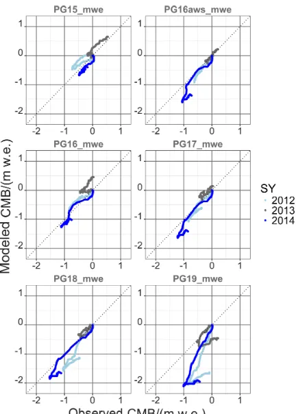
loca-Figure 10.Cumulative mass balance (CMB) from simulations with the glacier melt model (modelled CMB) and observation (observed CMB) on the Warszawa Icefield (transect ID PG0x) for calibration purposes. Year numbers give the year of start of the glaciological mass balance year. It encompasses the glaciological years 2012/13 to 2014/15.
tions PG05 and PG08 (Fig. 8) and PG15 and PG18 (Fig. 9). The GMM outputs the cumulative accumulation and ablation for 10 m by 10 m grid cells at the stake locations. Model cal-culations are shaded in grey. Figures 8 and 9 show that model and observations are generally in agreement. The GMM does not fully account for the spread in the observations, which is attributed to the significant snow drift due to high wind speeds and snow deposit due to turbulence at the glacier end moraine and to the high contribution of snow erosion by rain. Figures 10 and 11 show the high interannual variability. The high frequency of observations allows one to differenti-ate between periods with different climatic settings. The high deviation of CMB, especially towards the end of the abla-tion period, shows that the GMM clearly underestimates the accumulation due to snow drift and turbulence-driven snow deposition at the glacier border (see Figs. 10 and 11). The closer the MBSs are to the glacier border, the more the effect of turbulence-driven snow deposition comes into effect.
Figure 11.Cumulative mass balance (CMB) from simulations with the glacier melt model (modelled CMB) and observation (observed CMB) on the Warszawa Icefield (transect ID PG1x) for validation purposes. Year numbers give the year of start of the glaciological mass balance year. It encompasses the glaciological years 2012/13 to 2014/15.
below freezing and snow fall occurred together with high wind speeds. This leads to an underestimation in the simu-lated CMB since the GMM does not account for snow drift. Then there is a period when model and observations are in very good agreement. During the fall of SY 2014, there were frequent rain events. Since the GMM was run in catchment configuration, meaning that the model area contained also the periglacial parts of the hydrological catchment, the snow module (Reijmer and Hock, 2008) could not be applied. Re-freezing processes could, thus, not be considered, and the simulated CMB is also underestimated. The accumulation period at the end of SY 2014 is again marked with the un-derestimation in CMB due to the disregard of snow drift in the GMM.
Apart from these two climatic boundary conditions, the model results and the glaciological observations are in good agreement, and a drift or disagreement over the 5-year GMM run period cannot be seen in the data.
Table 2.Definition of beginning and end of the glaciological sum-mer deducted from observations of local minima and maxima of the accumulation/ablation time series at the mass balance transects (PG0xand PG1x) on Potter Peninsula, King George Island, during the time period November 2010 to December 2016.
Glaciological Begin of Begin of
year ablation period accumulation period
Year Day of year Year Day of year
2010/11 2010 345 2011 103
2011/12 2011 335 2012 85
2012/13 2012 315 2013 139
2013/14 2013 275 2014 74
2014/15 2014 344 2015 126
2015/16 2015 331 2016 110
2016/17 2016 352
4.2 Glacier surface mass balance
Cogley et al. (2011) give the annual (surface) mass balance (bn) at the end of a balance year as the sum of winter mass
balance (bw), i.e. the sum of winter accumulation (cw) and
ablation (aw), and summer mass balance (bs), i.e. the sum of
summer accumulation (cs) and ablation (as):
bn=cw+aw+cs+as=bw+bs. (15)
All mass balances calculated here refer to the points of the MBS transects and are referred to by lowercase letters (b). Ice density is assumed to be ρice=900 kg m−3 equivalent
to 0.9 kg L−1. All units are in kg m−2. Assuming an uncer-tainty in snow height measurements of1H=0.2 m to ac-count for natural surface heterogeneity around each stake and of1ρ=10 kg m−3for the variability in snow density mea-surements leads to an uncertainty of1b=0.35 m w.e. in spe-cific glacier mass balance estimates.
Figure 12.Specific summer, winter and net mass balance (bs,bn and bn, respectively) in m w.e. derived from mass balance stakes observation at transects PG0xduring 2010 to 2016.
The glaciological year 2011/12 contained a very cold and dry winter in 2011. The summer 2012 showed an exception-ally high net radiation balance amounting to 156 % of the seasonal 5-year average. The resulting high ablation entails a strongly negative specific net balance. In July of winter 2012 brought a 2-week period of rain together with above freezing air temperatures, leading to the erosion of the fresh snow pack and to low accumulation in the net balance. Al-though the summer 2013 showed low ablation due to high cloud coverage and less precipitation, the glaciological year 2012/13 remains in its net balance negative. It was also a year with very low winds during summer and very high winds during winter. The glaciological year 2013/14 reveals a wet winter with high accumulation rates but also a very cold and very wet summer resulting in low ablation. Regardless of this, the net balance was negative. The glaciological year 2014/15 started with a warm and wet winter, followed by a warm and dry summer leading to higher ablation rates. The period of 2015/16 was a very strong El Niño year with a very cold winter in 2015, followed by a warm and very long sum-mer in 2016. The MSB PG19 (at the elevation of ca. 100 m) clearly reflects the effect of turbulence-driven snow accumu-lation at the glacier end moraine. Estimates of bn are
sig-Figure 13.Specific summer, winter and net mass balance (bs,bw andbn, respectively) in m w.e. derived from mass balance stakes observation at transect PG1xduring 2010 to 2016.
nificantly higher than the GMM output for this stake loca-tion. The variability and impact of snow drift and turbulence-driven snow deposition is evident in the locally calculated estimates ofbn of the MBS observations. From the graphs
(Figs. 12 and 13), it becomes clear that winter accumulation is in most of the years not sufficient to cover for the summer ablation. Summer ablation or the specific summer mass bal-ance, in contrast, is revealed to be highly variable between years, depending on climatic conditions and the length of the ablation period of the respective glaciological year.
4.3 Meltwater discharge into Potter Cove
The GMM calculates the discharge on an hourly basis ac-cording to the temporal resolution of the meteorological in-put time series. The GMM configuration allows for comin-puta- computa-tion of partly glaciated catchment areas as is the case for the Potter Cove catchment. The GMM differentiates between the source areas of the meltwater discharge:
qsim=qfirn+qsnow+qice+qrock+qground. (16)
Figure 14.Time series of meltwater discharge from GMM run November 2010 to November 2015 for the Fourcade Glacier, catchment of the Potter Cove, separated into the different source areas (AID) of snow, firn, ice and rock terrain (qsnow, qfirn, qiceandqrock). The complete simulated meltwater discharge (qcalc) is shown in black solid circle with the standard deviation of the time series in grey envelope.
and the respective source areas (firn, ice, snow and rock). The penetration and discharge through ground is negligible, qground≈0. Area sizes change over the course of a year.
Figure 14 shows the transitional importance of the dominat-ing source area to glacial discharge throughout the seasons. The contribution of firn areas to glacial discharge is mainly controlled by the seasonal course of surface air temperature and net radiation balance. Since the albedo for firn areas re-main high during the summer (α >0.75), firn surface melt starts in spring and consistently pertains throughout the sum-mer with monthly discharge quantities of<0.5 m3s−1. The glaciological year 2014/15 contained a very cold and mod-erately wet winter followed by a very warm but dry sum-mer. This resulted in a pronounced time lag between snow and ice area contribution to glacial discharge but also high meltwater quantities due to the amount of winter precipita-tion. Glacial discharge from snow areas predominate the first part of a summer season and from ice areas in the second part. Differences in monthly discharge from snow areas can amount to nearly 1 m3s−1between years. The high variabil-ity of ablation and accumulation reflects the very high inter-and intra-annual variability of the meteorological boundary conditions (Falk and Sala, 2015a). The frequent occurrence of melt periods during winter is attributed to advection of moist and warm air masses from mid-latitudes by synoptic low-pressure systems. This results in non-zero discharge for winter season (JJA: June to August). Figure 15 shows the
sea-Figure 15.Seasonal meltwater discharge from GMM run for the Fourcade Glacier, a hydrological catchment of the Potter Cove (DJF: austral summer December–February; MAM: austral fall March–May; JJA: austral winter June–August; SON: austral spring September–November).
sonal sums of glacial discharge from Fourcade Glacier into Potter Cove as sums.
Linearly relating the time series of simulated discharge to the positive degree day (PDD) time series derived from the Carlini air temperature series (Falk and Sala, 2015a) shows a high correlation coefficient:
Figure 16. Equilibrium line altitude calculated from observations at transects PG0x(black, solid circle) and PG1x(black, solid tri-angle) and from GMM simulation (M) output at transects pixels PG0x(red, solid circle) and PG1x(red, solid triangle) for the time period 2010 to 2016. The 5-year average ELA from MBS obser-vations (MBS obs) and from GMM model results (GMM) are dis-played with the grey shading indicating the uncertainty around the average observed ELA.
This means that 84 % of the changes in discharge can be explained by changes in air temperature. Observed tempera-ture trends are highest in winter months, i.e. a trend in min-imum air temperature of nearly 5◦C over four decades for August (Falk and Sala, 2015a). This might result in lesser accumulation during winter and, thus, in a more negative mass balance. The linear regression between the simulated discharge to the PDD time series calculated from the AWS data shows a lesser correlation:
qsim=0.4+0.14·PDD, R2=0.74. (18)
Above glaciated areas, surface air temperature is being re-duced by the melt processes. Thus, PDD and degree day fac-tor analysis are best derived from air temperature observa-tions that are within the catchment area but on non-glaciated areas.
The observed trend in SAM and surface air temperature es-pecially during wintertime (Falk and Sala, 2015a) can lead to significant glacial discharge within the winter season. Glacier facies with bare-ice conditions promote enhanced glacial dis-charge (see Fig. 14). The dark material, periodically resurfac-ing in the ablation area, significantly changes albedo to val-uesα <0.1 and, thus, reinforces the effect on surface melt. Hence, winters with missing or lesser accumulation can be expected to be followed by summers with higher rates of glacier discharge.
Figure 17.Equilibrium line altitude estimates from this study (PG) and former glaciological studies during the last decades. ELA es-timates taken from literature encompass: BD is Bellingshausen Dome, KGI (Orheim and Govorukha, 1982; Jiahong et al., 1994; Jiawen et al., 1995); EG is Ecology Glacier, KGI (Bintanja, 1995); LI is Livingston Island (Vilaplana and Pallàs, 1994; Molina et al., 2007; Navarro et al., 2009, 2013); NI is Nelson Island (Jiawen et al., 1995); SG is Stenhouse Glacier, KGI (Curl, 1980); SSI is South Shetland Islands (Serrano and López-Martínez, 2000).
5 Discussion
Time series of accumulation and ablation show a very high intra- and interannual variability that concurs with the clima-tological variability that is reported by Falk and Sala (2015a). The observations at two mass balance stake transects demon-strate the high spatial variability, regular occurrence of win-ter melt periods and the impact of snow drift, turbulence-driven snow deposition, snow layer erosion by rain and high exposition to synoptic impact. These processes are not yet included in the model physics and can lead to discrepan-cies between GMM simulation and observations under spe-cific climatic conditions. Overall, observations and model are in good agreement though. The high interannual variability in climate conditions, accumulation and ablation patterns is propagated to variability in glacial discharge time series. The difference between years can be as high as 40 %. The simu-lated glacier discharge is highly corresimu-lated to PDD time se-ries with a coefficient of determination ofR2=0.84.
Figure 18.Glacier extent for equilibrium with actual climatic boundary conditions and an ELA of 260 m (pink line) for the Potter Cove catchment on KGI, according to an AAR between 0.5 (yellow line) and 0.8 (orange line). The actual glacier extent is marked as green and light blue line and represents our own differential GPS measurements in austral summer 2012/13 and 2016/17.
Figure 16 shows the ELA estimates from observations (black) at the transects PG1xand PG0x and from the GMM output (red). Error bars are derived from the regressions. The calculated ELAs are generally around 260 m altitude. Curl (1980) states that all glaciers on KGI appear in near-equilibrium and slightly negative conditions and that geolog-ical evidence shows no major detectable advance within the past two centuries. Braun and Gossmann (2002) have com-piled values of the ELA obtained by different authors in the South Shetland Islands region along the last decades. Jiawen et al. (1995) do not give uncertainties of their glaciological observations and ELA estimates but state that a high vari-ability between different consecutive years was observed. Ji-ahong et al. (1994) and JiJi-ahong et al. (1998) concluded from mass balance studies on Collins or Bellingshausen Dome that this small ice cap was in steady state between 1971 and 1991 in agreement with Curl (1980). Serrano and López-Martínez (2000) presented a concurrent ELA for the South Shetland Islands located around 165 to 250 m a.s.l.Bintanja (1995) asserted that the ELA was around 100 m in the Ecol-ogy Glacier, KGI. Despite the strong variability, the ELA has increased by more than 100 m from the late 1960s up to the 1990s. More recently Osmanoglu et al. (2014), Navarro et al. (2013, 2009) and Molina et al. (2007) have placed the ELA
at∼230 m and∼187 m for Hurd and Johnsons glaciers, re-spectively, both located at Livingston Island ice cap.
to 260±20 m and is displayed in Fig. 16 as a dot-dashed line with the uncertainty in grey shading.
Figure 17 places the results from our own glaciological ob-servations into the long-term context. Where available, error or uncertainty bars were included. The temporal evolution of the ELA estimates from the different glaciological studies show clearly that until the 1980s the glaciers on KGI were in near-equilibrium (Curl, 1980), but after this time period there is a clear increase in the ELA. Our analysis in the preceding paragraphs shows not only that the accumulation of Fourcade Glacier generally does not suffice to account for the ablation but also that the interannual variability is high especially dur-ing the ablation period. The Fourcade Glacier is clearly in retreating mode, also due to the fact that ice flow velocities in lower glacier on Potter Peninsula are below 1 m yr−1(Falk et al., 2016). The ice mass flux cannot compensate the melt losses in the ablation zone.
The expected ratio of accumulation area to the total glacierized area for a glacier in equilibrium with its climate (AAReq) is within the range of 0.5 to 0.8, e.g. Meier and Post
(1962) and Paterson (1994). Corresponding to the observed average ELA of 260 m with concurrent glacier extent is a ra-tio of approx. 0.26 for the Potter Cove catchment, meaning the glacier is clearly retreating until it reaches its equilibrium state shown in Fig. 18. Here, the yellow line marks the glacier extent for elevations above 110 m referring to an AAR=0.8 and the orange line marks the glacier extent for elevations above 230 m referring to an AAR of 0.5. Underlying is the assumption that lower elevations will melt homogeneously and ice velocities are negligible as soon as the glacier termi-nates on land in the Potter Cove catchment.
6 Conclusions
One of the most intuitive parameters to describe the equi-librium state of a glacier is the AAR, meaning the state and health of a glacier. Particularly, it is an indicator for expected future retreat or growth of a glacier until it gets into equilib-rium with concurrent climatic conditions. It thus relates via the ELA with the specific mass balance and changes of total glacier area. The more negative the mass balance, the higher the elevation line of ELA and the smaller the AAR. Once the long-term ELA reaches values higher than the maximum altitude of the glacier dome, there is no more accumulation area and the glacier will disappear sooner or later. Möller and Schneider (2015) define this as the turning or tipping point of the glacier evolution.
This behaviour also depends on the bedrock topography, which remains largely unknown for the Warszawa Icefield. If underneath the glacier is mountainous terrain, then the stratigraphy of glacier ice mass would persist longer due to higher elevation than if it would all be ice mass underneath. Glaciers respond to climatic boundary conditions with a time lag of a few decades to centuries until they are in
equilib-rium with the climatic conditions (Paterson, 1994). The al-ready committed mass change will lead to further retreat of the glacier border within the near future.
A tipping point will be reached for the glacier when the ELA rises above the highest point of the glacier which im-plies that the accumulation area goes to zero, i.e. an ELA> 490 m. Even if the observed trends in climatic boundary con-ditions do not continue, the Fourcade Glacier would still re-treat until it reaches equilibrium with climatic conditions. Its extent will be defined by these conditions and the glacier border located between the yellow and the orange line in Fig. 18. The equilibrium state corresponds to a glacier ex-tent that would approximately end between the elevation lines ofhelev=110 m (Fig. 18 yellow line) andhelev=230 m
(Fig. 18 orange line), referring to an AAReqof 0.8 and of 0.5,
respectively. Thus, further retreat of the glacier border is to be expected. The southern part of the Fourcade Glacier on Pot-ter and on Barton Peninsula contains a major area of very low ice flow velocities<1 m2and below the ELA in the ablation zone. These areas can be assumed to decrease the most and the glacial meltwater streams are likely to significantly in-crease their sediment freight due to larger distances through moraine landscape.
The high variability in melt conditions and in especially missing winter accumulation is found to enhance glacial discharge. Positive air temperatures and thus non-frozen moraine landscape surface also promote the intake of sedi-ment load into the meltwater streams that is then introduced into the coastal waters. Assuming the most extreme sce-nario of glacial retreat according to the ELA–AAR analysis (Fig. 18), the length of meltwater streams through moraine landscape could increase by as much as three times the cur-rent stream length, expecting to pick up more sediment load in the near future. This would increase changes in physi-cal and chemiphysi-cal properties of coastal environments, hence leading to a higher impact on the biological communities. Considering the high adaptation required for Antarctica’s ex-treme environments, the high seasonal and interannual vari-ability in climatic and glacial melting conditions can be as-sumed to have a direct impact on coastal ecosystems.
Code availability. All R codes are available on request from Ulrike Falk.
Data availability. Supplementary data are available at https://doi.org/10.1594/PANGAEA.874599 (Falk et al., 2017) and https://doi.org/10.1594/PANGAEA.848704 (Falk and Sala, 2015b).
project. DL was responsible for the quality assessment and control of mass balance data time series, the establishment of final glacio-logical protocols and all communication with the overwinterers. All final analysis and post-processing of climatological and glaciologi-cal data time series was performed by UF. ASB investigated the hy-drology of Potter Cove and refined the catchment definition grids for the glaciological surface mass balance model. Glaciological mod-elling work was carried out by UF, with ASB contributing to the calibration and validation procedures. The manuscript was mainly written by UF. DL contributed to the sections concerning mass ance stake observations and analysis, as well as glacier mass bal-ance. ASB wrote parts for the hydrological catchment definition and contributed to the sections on glacier discharge and meltwater anal-ysis.
Competing interests. There are no potential conflicts of interest re-garding financial, political or other matters.
Acknowledgements. We would like to thank the Alfred Wegener In-stitute (AWI) from Germany and the Instituto Antártico Argentino – Dirección Nacional del Antártico (IAA-DNA) from Argentina for their support in Antarctica. A special acknowledgement goes to Hernán Sala for assistance in the field and help with logistics and to the overwintering scientists at Carlini Station and Dallmann Laboratory: Daniel Viqueira, Juan Piscicelli, Facundo Alvarez, Francisco Ferrer, Pablo Saibene, Martín Gingins and Julia Luna without whom this work would not have been possible. During the period 2010–2015, the overwintering crews from the Ejército Argentino at Carlini Station continuously supported our scientific tasks and we would like to specifically mention SP Norberto Leonardo Galván. We also than Regine Hoch and the University of Fairbanks in Alaska for the introduction to the glacier melt model. All graphs in this paper were produced using the R programming language (R Core Team, 2014) and QGIS software (QGIS Devel-opment Team, 2016). We also thank the funding support provided by the ESF ERANET Europolar IMCOAST project (BMBF award AZ 03F0617B) and the Marie Curie Action IRSES (FP7 IRSES, action no. 318718), the logistic support by the Universities of Bonn, Bremen and Erlangen-Nuremberg and the Argentinean Antarctic Institute (IAA-DNA). We thank Ben Marzeion for the careful reading of and his very helpful comments on the manuscript.
The article processing charges for this open-access publication were covered by the University of Bremen.
Edited by: Thomas Mölg
Reviewed by: two anonymous referees
References
AARI: Meteorological observations at Bellingshausen, Arctic and Antarctic Research Institute, St. Petersburg, Russia, available at: http://www.aari.nw.ru/index_en.html, last access: 1 January 2016.
Abele, D., Vazquez, S., Buma, A., Hernandez, E., Quiroga, C., Held, C., Frickenhaus, S., Harms, L., Lopez, J., Helmke, E.,
and Mac Cormack, W. P.: Pelagic and benthic commu-nities of the Antarctic ecosystem of Potter Cove: Ge-nomics and ecological implications, Mar. Genom., 33, 1–11, https://doi.org/10.1016/j.margen.2017.05.001, 2017.
Abram, N., Thomas, E. R., McConnell, J. R., Mulvaney, R., Bracegirdle, T. J., Sime, L. C., and Aristarain, A.: Ice core evidence for a 20th century decline of sea ice in the Bellingshausen Sea, Antarctica, J. Geophys. Res., 115, 9, https://doi.org/10.1029/2010JD014644, 2010.
Andreas, E.: IA theory for the scalar roughness and the scalar trans-fer coefficients over snow and sea ice, Bound.-Lay. Meteorol., 38, 159–184, 1987.
Barrand, N., Vaughan, D., Steiner, N., Tedesco, M., Kuipers Munneke, P., Broeke, M., and Hosking, J.: Trends in Antarctic Peninsula surface melting conditions from obser-vations and regional climate modeling, J. Geophys. Res.-Earth, 118, 315–330, 2013.
Bintanja, R.: The local surface energy balance of the Ecology Glacier, King George Island, Antarctica: mea-surements and modelling, Antarct. Sci., 7, 315–325, https://doi.org/10.1017/S0954102095000435, 1995.
Birkenmajer, K.: Retreat of Ecology Glacier, Admiralty Bay, King George Island (South Shetland Islands, West Antarctica), 1956– 2001, B. Pol. Acad. Sci.-Earth, 50, 15–29, 2002.
Bishop, M. P., Olsenholler, J. A., Shroder, J. F., Barry, R. G., Raup, B. H., Bush, A. B., Copland, L., Dwyer, J. L., Foun-tain, A. G., Haeberli, W., Kääb, A., Paul, F., Hall, D. K., Kargel, J. D., Molnia, B. F., Trabant, D. C., and Wessels, R.: Global Land Ice Measurements from Space (GLIMS): remote sensing and GIS investigations of the Earth’s cryosphere, Geocarto Int., 19, 57–84, 2004.
Braun, M. and Gossmann, H.: Glacial Changes in the Areas of Admiralty Bay and Potter Cove, King George Island, Maritime Antarctica, Springer, Berlin Heidelberg, 75–89, 2002.
Braun, M. and Hock, R.: Spatially distributed surface energy bal-ance and ablation modelling on the ice cap of King George Island (Antarctica), Global Planet. Change, 42, 45–58, 2004.
Braun, M., Humbert, A., and Moll, A.: Changes of Wilkins Ice Shelf over the past 15 years and inferences on its stability, The Cryosphere, 3, 41–56, https://doi.org/10.5194/tc-3-41-2009, 2009.
Braun, M., Betsch, T., and Seehaus, T.: King George Island TanDEM-X DEM, link to GeoTIFF, Geo-graphic Institute, Universitaet Erlangen-Nuernberg, https://doi.org/10.1594/PANGAEA.863567, 2016.
Brock, B. W., Willis, I. C., and Sharp, M. J.: Measurement and parameterization of aerodynamic roughness length variations at Haut Glacier d’Arolla, Switzerland, J. Glaciol., 52, 281–297, 2006.
Bromwich, D. H., Rogers, A. N., Kållberg, P., Cullather, R. I., White, J. W., and Kreutz, K. J.: ECMWF analyses and reanalyses depiction of ENSO signal in Antarctic precipitation, J. Climate, 13, 1406–1420, 2000.
Campbell, G. S. and Norman, J. M.: Environmental Biophysics, 2nd Edn., Springer, New York, Berlin, Heidelberg, 2000.