www.atmos-meas-tech.net/7/1901/2014/ doi:10.5194/amt-7-1901-2014
© Author(s) 2014. CC Attribution 3.0 License.
Water vapor retrieval from OMI visible spectra
H. Wang1, X. Liu1, K. Chance1, G. González Abad1, and C. Chan Miller2 1Harvard-Smithsonian Center for Astrophysics, Cambridge, MA 02138, USA
2Department of Earth and Planetary Sciences, Harvard University, Cambridge, MA 02138, USA
Correspondence to: H. Wang (hwang@cfa.harvard.edu)
Received: 2 December 2013 – Published in Atmos. Meas. Tech. Discuss.: 22 January 2014 Revised: 21 April 2014 – Accepted: 23 May 2014 – Published: 30 June 2014
Abstract. There are distinct spectral features of water vapor in the wavelength range covered by the Ozone Monitoring Instrument (OMI) visible channel. Although these features are much weaker than those at longer wavelengths, they can be exploited to retrieve useful information about water vapor. They have an advantage in that their small optical depth leads to fairly simple interpretation as measurements of the total water vapor column density. We have used the Smithsonian Astrophysical Observatory (SAO) OMI operational retrieval algorithm to derive the slant column density (SCD) of wa-ter vapor using the 430–480 nm spectral region afwa-ter exten-sive optimization. We convert from SCD to vertical column density (VCD) using the air mass factor (AMF), which is calculated using look-up tables of scattering weights and as-similated water vapor profiles. Our Level 2 product includes not only water vapor VCD but also the associated scatter-ing weights and AMF. In the tropics, our standard water va-por product has a median SCD of 1.3×10²³molecules cm−2 and a median relative uncertainty of about 11 %, about a fac-tor of 2 better than that from a similar OMI algorithm that uses a narrower retrieval window. The corresponding median VCD is about 1.2×10²³molecules cm−2. We have exam-ined the sensitivities of SCD and AMF to various param-eters and compared our results with those from the Glob-Vapour product, the Moderate Resolution Imaging Spec-troradiometer (MODIS) and the Aerosol Robotic NETwork (AERONET).
1 Introduction
Water vapor is one of the key factors for weather. It is also the most abundant greenhouse gas in the atmosphere. It can pro-vide strong feedback directly through amplification of global
warming associated with other greenhouse gases and indi-rectly through formation of clouds. Water vapor participates in many photochemical reactions, such as the reaction with O(1D) to produce OH radicals, which control the oxidation capacity of the atmosphere. It is therefore also important for atmospheric chemistry. Unlike other long-lived greenhouse gases, the short-lived water vapor exhibits large spatial and temporal variability. Monitoring the distribution, variability and long-term changes in water vapor is critical for under-standing the hydrological cycle, the earth radiative budget and climate change.
400 420 440 460 480 500 Wavelength (nm)
0 2 4 6 8
Reference Spectra
H2O
O3 NO2
C2H2O2
O2-O2
Liquid_H2O
Ring
Water_ring
Figure 1. Reference spectra used in the standard operational water vapor retrieval. The spectra have been scaled for presentation pur-poses. The black lines are those listed in Table 1. The red lines are the black lines convolved with the OMI slit function.
Wagner et al. (2013) demonstrated the feasibility of wa-ter vapor retrieval in the blue spectral range using GOME-2 and Ozone Monitoring Instrument (OMI) measurements. They pointed out that the advantages of this spectral range in-clude more consistent retrievals across the globe due to more uniform surface albedo, especially between land and ocean, increased sensitivity to near-surface layer due to higher sur-face albedo over the oceans than for longer wavelengths, less saturation of signal due to weaker water vapor absorption, applicability to sensors that do not cover longer wavelengths, and daily global coverage over a long period of time.
Wagner et al. (2013) derived OMI water vapor slant col-umn densities (SCDs). We have independently derived OMI water vapor SCDs and converted them to vertical column densities (VCDs) using the Smithsonian Astrophysical Ob-servatory (SAO) operational retrieval algorithm. In this pa-per, we will present our SCD retrievals, VCD calculations, sensitivity studies and initial validation results.
2 Data processing
2.1 OMI instrument and OMI data
OMI is a joint Dutch–Finnish instrument onboard the NASA EOS-Aura satellite, which was launched on 15 July 2004 into a sun-synchronous orbit with an ascending node Equa-tor crossing time of around 13:45 LT and an orbital period of about 100 min (Schoeberl et al., 2006). It is a nadir-viewing push-broom ultraviolet/visible (UV/VIS) imaging spectrom-eter with three channels – the UV1 (264–311 nm), UV2 (307–383 nm) and VIS (349–504 nm) – at 0.42–0.63 nm spectral resolution (Levelt et al., 2006). For the visible chan-nel, the 2600 km OMI cross-track swath usually provides a nominal spatial resolution between 13 km×24 km at nadir and 26 km×135 km at the edge. The entire globe is covered by 14–15 orbits each day. Solar irradiance measurements are performed daily.
We use Version 3 Level 1B OMI visible spectra to derive water vapor SCD, and Version 3 Level 2 OMI cloud pressure and cloud fraction product (OMCLDO2) downloaded from disc.sci.gsfc.gov/Aura/data-holdings/OMI/ for air mass fac-tor (AMF) calculation.
2.2 Slant column retrieval 2.2.1 Standard retrieval
We determine the slant column of water vapor by directly fitting the OMI spectra following the method described in Chance (1998). The method is also presented in detail in González Abad et al. (2014). In this paper, we only provide a brief description.
are interpolated onto common calibrated radiance grid and convolved with pre-determined instrument slit function (Dirksen et al., 2006) during the fitting (Fig. 1). Ozone, nitrogen dioxide, water vapor and glyoxal are corrected for the solarI0effect (Aliwell et al., 2002).
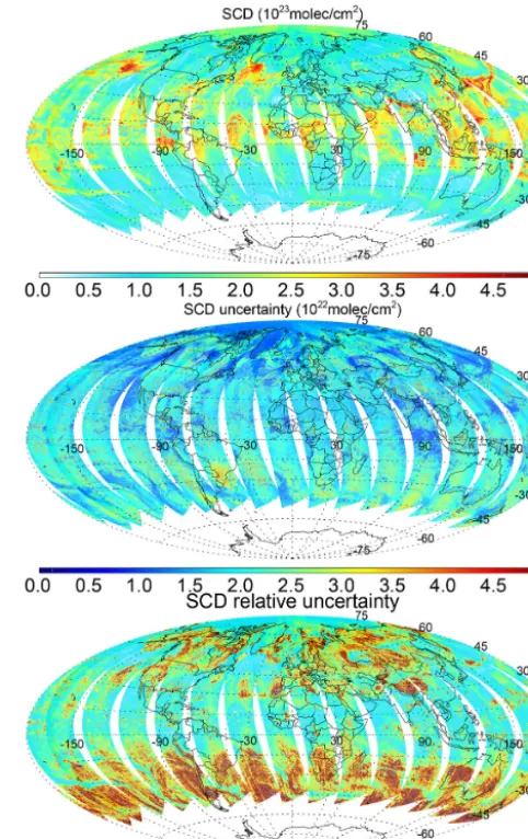
Figure 2 shows our standard retrieval result for the SCD and the associated absolute and relative uncertainties for 14 July 2005 (orbits 5297–5311). As expected, the global pattern shows more water vapor in the Intertropical Conver-gence Zone (ITCZ) and mid-latitude weather systems. There are some stripes along the swaths (Veihelmann and Kleipool, 2006) as we have not applied our post-processing routine to remove them for this plot. The stripes are mainly caused by OMI systematic measurement errors and are common to most OMI Level 2 products. In the tropics (30◦S–30◦N), the median of SCD is 1.32×10²³ molecules cm−2, the median of fitting uncertainty is 1.2×10²²molecules cm−2, the me-dian of relative uncertainty (fitting uncertainty/SCD) is 11 % and the median of the fitting root mean square (rms) ratio to the radiance is 9.2×10⁻⁴. Areas with larger SCD generally have smaller uncertainties.
The 25 % and 75 % percentiles of our fitting uncertainties in the tropics are 1.0×10²²and 1.7×10²²molecules cm−2, respectively. In comparison, using a shorter retrieval window of 430–450 nm, Wagner et al. (2013) obtained typical SCD uncertainties of 3–5×10²²molecules cm−2for OMI and 1– 2.5×10²²molecules cm−2for GOME-2. The uncertainty of our standard water vapor SCD is therefore smaller than the Wagner et al. (2013) OMI result and similar to the Wagner et al. (2013) GOME-2 result.
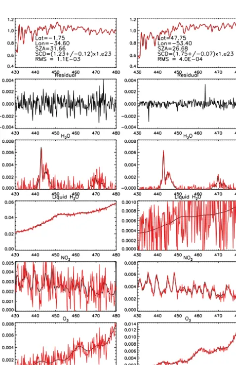
Figure 3 shows examples of our spectral fitting for two pixels from orbit 5306 in July 2005. The left col-umn is for a pixel at 1.75◦S and 34.6◦W in the Atlantic
Ocean, and the right column is for a pixel at 47.75◦N and 53.4◦W at the Atlantic coast of North America. The retrieved water vapor SCDs are (1.23×0.12)×1023 and (1.75×0.07)×1023molecules cm−2, respectively. The cor-responding rms values are 1.1×10⁻³ and 4.0×10⁻⁴, re-spectively. The panels in the top row show that the fitted spectra (red) closely track the measured spectra (black). The panels in the second row show that the fitting residuals ap-pear random except for two minor noise spikes in the right-hand spectrum. The next four rows show the reference spec-tra of important molecules (water vapor, liquid water, nitro-gen dioxide and ozone) scaled by their corresponding fitted SCDs (black) and added to the fitting residuals in the second row (red). In both cases, the water vapor spectral signature within the fitting window is stronger than the fitting residu-als. Consistent with the expectation that there is less liquid water, more NO2 and more O3 in the mid-latitude coastal area than in the tropical open ocean, the right panels show that the liquid water signal is weaker and the NO2 and O3 signals are stronger than the residual, while the left panels show the opposite.
Figure 2. OMI water vapor (top) SCD, (middle) SCD uncertainty and (bottom) SCD relative uncertainty for 14 July 2005 from the standard retrieval.
2.2.2 Sensitivity studies
Table 1. Reference spectrum used in standard retrieval.
Molecule T (K) Reference
Water vapor (H2O) 280 Rothman et al. (2009) Ozone (O3) 228 Brion et al. (1993) Nitrogen dioxide (NO2) 220 Vandaele et al. (1998)
Oxygen collision complex (O2-O2) 294 http://spectrolab.aeronomie.be/o2.htm Pure liquid water (H2O) – Pope and Fry (1997)
Glyoxal (C2H2O2) 296 Volkamer et al. (2005) Ring and water ring – Chance and Spurr (1997)
Figure 3. Spectral fitting results for (left) a pixel in the Atlantic Ocean and (right) a pixel near the Atlantic coast of North America. The first row shows the fitted (red) and measured (black) spectra. The second row shows the fitting residuals. The third to sixth rows show the reference spectra of H2O, liquid water, NO2and O3scaled by the fitted slant columns (black) and added to the fitting residuals (red).
25 % larger. The median SCD decreases from 1.47×10²³to 1.23×10²³molecules cm−2 as the retrieval window length increases.
We have performed additional sensitivity studies, shown in Table 3, by excluding the interfering molecules, changing the reference spectra and changing the order of closure polyno-mials. In these experiments, everything else is kept the same as in the standard retrieval. In Table 3, we list the median statistics and the number of negative retrievals for water va-por between 30◦S and 30◦N for 14 July 2005.
Exclusion of O3, O2–O2, NO2 or liquid water leads to significant (10–30 %) reduction of the retrieved water vapor SCDs and large increase of the number of negative retrievals, though the fitting uncertainties and rms remain at the same level. The most severe change is associated with liquid wa-ter, followed by NO2, O2–O2and O3. Exclusion of C2H2O2 leads to only about 1 % increase of water vapor SCD. With-out liquid water, the medium water vapor SCD decreases by about 32 % from 1.32×10²³to 0.90×10²³molecules cm−2, and the number of negative retrievals increases from 1935 to 50 216. It should be noted that such a strong sensitivity to liquid water is for the standard long retrieval window of 430–480 nm. For the shorter window of 432–462 nm, the dif-ference in the median SCD with and without liquid water is only about 4 %, which is substantially smaller than the me-dian relative uncertainty.
As a by-product of our standard water vapor retrieval, the top panel of Fig. 4 shows the retrieved liquid water on 14 July 2005. Although the retrieval is not optimized for liquid water, areas in the oceans, seas, gulfs and so on are highlighted. Not all liquid water bodies are highlighted to the same extent. Comparison between the top and middle panels of Fig. 4 shows that some liquid water surfaces are shielded by clouds. The bottom panel of Fig. 4 shows the re-trieved water vapor SCD without considering liquid water. Compared to the standard retrieval shown in the top panel of Fig. 2, the SCDs here are apparently smaller, especially over the areas with liquid water where many negative values (plotted as blanks) are retrieved.
Table 2. Sensitivity to retrieval window.
Window Retrieval Median SCD Median uncertainty Median relative length (nm) window (nm) (molecule cm−2) (molecule cm−2) uncertainty
20 [435, 455] 1.47×10²³ 2.4×10²² 0.19 30 [432, 462] 1.43×10²³ 2.0×10²² 0.17 40 [438, 478] 1.35×10²³ 1.6×10²² 0.15 50 (standard) [430, 480] 1.32×10²³ 1.2×10²² 0.11 65 [430, 495] 1.23×10²³ 1.5×10²² 0.12
Table 3. Miscellaneous sensitivity studies.
Description Median SCD Median uncertainty Median Number of
(molecule cm−2) (molecule cm−2) rms negatives
Standard 1.32×10²³ 1.2×10²² 9.2×10⁻⁴ 1935
Without O3 1.19×10²³ 1.2×10²² 9.3×10⁻⁴ 7234
Without O2-O2 1.18×10²³ 1.3×10²² 9.9×10⁻⁴ 5076
Without NO2 1.05×10²³ 1.2×10²² 9.3×10⁻⁴ 15666
Without liquid water 0.90×10²³ 1.1×10²² 9.5×10⁻⁴ 50216
Without C2H2O2 1.34×10²³ 1.2×10²² 9.2×10⁻⁴ 1780
Switch to fifth-order polynomial 1.32×10²³ 1.3×10²² 9.0×10⁻⁴ 2262 Switch reference H2O to 0.7 atm and 265 K 1.29×10²³ 1.2×10²² 9.2×10⁻⁴ 1992 Switch reference H2O to 1.0 atm and 288 K 1.34×10²³ 1.2×10²² 9.2×10⁻⁴ 1918 Switch to Rothman et al. (2013) HITRAN 2012 water vapor 1.24×10²³ 1.2×10²² 9.2×10⁻⁴ 1816 Switch to Thalman and Volkamer (2013) O2-O2 1.31×10²³ 1.2×10²² 9.2×10⁻⁴ 2185
land. The common mode for each orbit is derived from the average of the fitting residuals. The fitting program then uses the derived common mode as a reference spectrum for the final retrieval. Since common mode is fitted, the change in the median fitting rms in Table 3 is small. Further exclusion of the common mode from the retrieval without liquid wa-ter will lead to an increase of the median rms for the day from 9.5×10⁻⁴ to 1.13×10⁻³. The common modes for the retrieval without liquid water are shown in the second row. There are apparent spectral structures in the common mode for the ocean-dominated Orbit 5311. In comparison, the common appears more random for the land-dominated Orbit 5304. The median rms in this case is 9.7×10⁻⁴for Orbit 5311 and 8.5×10⁻⁴for Orbit 5304. When liquid wa-ter is included in the retrieval, the bottom row shows that the spectral structures of the common mode for Orbit 5311 are reduced while those for Orbit 5304 are little affected. The median rms for the standard retrieval is 9.4×10⁻⁴for Orbit 5311 and 8.4×10⁻⁴ for Orbit 5304. The remaining struc-tures in the common mode of the standard retrieval over the ocean probably suggest errors in the liquid water reference spectrum. This will be investigated further in the future.
After obtaining new reference spectra for water vapor and oxygen collision complex, we have tested the sensitivity of our standard retrieval with respect to them. Switching from HITRAN 2008 (Rothman et al., 2009) to HITRAN 2012
(Rothman et al., 2013) water vapor reference makes the me-dian SCD about 6 % lower than that of the standard retrieval. In comparison, the median relative uncertainty of the stan-dard retrieval is about 11 %. Switching to the Thalman and Volkamer (2013) O2–O2reference spectrum gives almost the same result as the standard retrieval, so does switching from a third-order to a fifth-order closure polynomial for the base-line and scaling factor. The median of SCD retrieved using water vapor reference spectrum at 0.7 atm and 265 K is about 2 % lower than the standard result, and that using water vapor reference at 1.0 atm and 288 K is about 2 % higher. Due to the small changes in the SCD statistics, we have not updated the standard retrieval with the new reference spectra.
3 Vertical column calculation 3.1 AMF calculation
Figure 4. The top panel shows the liquid water index from a by-product of our standard water vapor retrieval. The middle panel shows the cloud fraction from the OMCLDO2 product. The bottom panel shows the water vapor SCD from a sensitivity study where liquid water is excluded from the water vapor retrieval. All results are for 14 July 2005.
the ratio of the scattering weights to the AMFs (Eskes and Boersma, 2003). Our Level 2 product provides VCDs with the scattering weights and AMFs for comparison with or as-similation into models. More details about the AMF calcu-lation for our operational retrieval algorithm can be found in González Abad et al. (2014).
The a priori vertical profiles of water vapor for the shape factor are from the monthly mean early afternoon GEOS-5 data assimilation product. They are generated at the Global Modeling and Assimilation Office (GMAO) and re-gridded to 2◦latitude×2.5◦longitude×47 layer resolu-tion (for GEOS-Chem simularesolu-tions). We use the monthly mean profiles in our operational retrieval to avoid the need
Figure 5. The top row shows the OMI VCDs for Orbit 5311, which is mostly over the ocean, and for Orbit 5304, which is mostly over the land. The middle row shows the common modes for the two orbits when liquid water is excluded from the standard retrieval. The bottom row shows the common modes for the two orbits from the standard retrieval, which includes liquid water.
of obtaining near-real-time water vapor assimilation product. The retrieved water vapor VCDs can be easily adjusted using the provided scattering weights when water vapor profiles of higher spatial and temporal resolution are used. As a repre-sentative example, the left panel of Fig. 6 shows the monthly and zonal mean water vapor profile at 10◦N in July 2007.
It can be seen that water vapor is highly concentrated near the surface where theefolding scale height is approximately 4 km.
Figure 6. The left panel shows a representative water vapor vertical profile in the tropics. The dotted line indicates the height of the 800 mb level. The right panel shows the scattering weight for a (solid line) clear and a (dashed) cloudy atmosphere where the modeled Lambertian cloud surface is at the 800 mb level.
weighted average of the clear and cloudy part (Martin et al., 2002). The radiative cloud fraction is calculated as the cloud fraction (f )weighted by the radiance intensity of the clear (Iclear) and cloudy (Icloud) scenes (φ=(1−f )·fI·Icloud
clear+f·Icloud, González Abad et al., 2014).
We use the effective cloud fraction and cloud pressure from the Version 3 Level 2 OMICLDO2 product, which is derived using the O2–O2 absorption band at about 477 nm (Stammes and Noordhoek, 2002; Acaretta et al., 2004; Stammes et al., 2008). In the cloud algorithm, a cloud is represented by a Lambertian reflector with an albedo of 0.8. Consequently, a thin cloud that fully covers an OMI pixel is represented by a small effective cloud fraction. In addition, the retrieved cloud height is mostly inside the cloud. To keep consistency with the OMCLDO2 product, we also model a cloud as a Lambertian surface with an albedo of 0.8.
As an example, the right panel of Fig. 6 shows the scat-tering weight for a clear (cloud fraction=0, solid line) and a cloudy (cloud fraction=1 at 800 mb, which is at a height of about 1.5 km, dashed line) scene under typical conditions. For a clear atmosphere, the scattering weight decreases to-ward the surface where most of the water vapor resides. For a cloudy atmosphere, the scattering weight shows a jump at the cloud level where the sensitivity immediately above in-creases due to enhanced multiple scattering and that below drops to zero due to cloud shielding.
3.2 AMF sensitivity
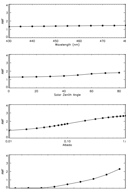
Since errors in AMF affect the quality of VCD, we in-vestigate the sensitivity of the AMF with respect to wave-length, solar zenith angle, surface albedo and cloud pressure
in Fig. 7. As a reference, we use a wavelength of 442 nm, sur-face albedo of 0.05, viewing zenith angle of 0◦, solar zenith angle of 30◦and surface height of 0 km. The top three panels of Fig. 7 correspond to a clear atmosphere, and the bottom panel corresponds to a cloudy atmosphere with cloud frac-tion of 1. We vary the parameters of interest one at a time to examine the AMF sensitivity.
The top panel of Fig. 7 shows that AMF is almost insensi-tive to wavelength. There is only about 1 % change over the 430–480 nm range. To speed up computation in our opera-tional retrieval, we use the AMF at 442 nm, which is within the strongest water vapor band in the 430–480 nm retrieval window. The second panel of Fig. 7 shows that the AMF in-creases from 1.25 to 1.85 as the solar zenith angle inin-creases from 0◦to 80◦. Since the viewing geometries of satellite ob-servations are precisely determined, errors due to this source can be neglected.
Figure 7. The variation of the AMF with respect to the wavelength, solar zenith angle, surface albedo and cloud height.
9 %. We will investigate the effect of using surface albedo database of higher spatial and temporal resolution (e.g., from MODIS) in the future.
Cloud is another factor that strongly affects AMF and VCD. The right panel of Fig. 6 shows that water vapor be-low the cloud is shielded from the view. As a result, AMF increases with increasing cloud top pressure (bottom panel of Fig. 7). The cloud product we use (OMCLDO2) is derived from O2–O2absorption band at about 477 nm. An alternative cloud product (OMCLDRR) is derived from rotational Ra-man scattering at about 350 nm (Joiner and Vassilkov, 2006). In both cases, the derived cloud pressure is different from that at the physical cloud top (Stammes et al., 2008; Vasilkov et al., 2008). A comparison by Sneep et al. (2008) shows that the differences in cloud pressure between them average be-tween 2 and 45 mb with an rms difference of 65 to 93 mb. Figure 7 shows that the AMF increases from 1.6 to 2.0 as the cloud pressure increases from 850 mb to 900 mb.
Aerosols influence atmospheric scattering and therefore AMF. There are different types of aerosols, and their distribu-tions are highly variable. This can potentially introduce sig-nificant error in AMF estimation. However, since the cloud product that we use does not consider aerosols, any effect as-sociated with aerosols is aliased into the cloud information. To be consistent, we do not consider aerosols in our radiative transfer calculation in this paper. In the future, we will per-form additional studies to better understand the influence of aerosols on our retrieval.
4 Validation
In this section, we present our initial data validation results. A comprehensive data validation will be performed later. In this paper, we compare our VCDs with the MODIS near-IR data, the GlobVapour MERIS+SSM/I combined data and the AERONET ground-based measurements.
The MODIS near-IR total precipitable water product (Gao and Kaufman, 2003) is derived using the ratios of water va-por absorbing channels (0.905, 0.936 and 0.94 µm) and atmo-spheric window channels (0.865 and 1.24 µm) in the near-IR. The retrieval algorithm relies on observations of water vapor attenuation of reflected sunlight. Therefore, results only exist for reflective surfaces in the near-IR. The errors are typically about 5–10 %, with greater errors over dark surfaces and un-der hazy conditions. Consequently, the data quality is gener-ally better over the land than over the ocean. In this paper, we use the Level 3 monthly 1◦×1◦data from the Aqua plat-form (MYD08_M3) (ladsweb.nascom.nasa.gov/data/). Aqua is about 15 min ahead of OMI’s host satellite Aura in the “A-train” constellation. Wang et al. (2007) found significant di-urnal cycles of precipitable water that vary with region and season. The closeness in local time of observation between OMI and MODIS is nice for comparison.
Figure 8. The first row shows the monthly mean 1◦×1◦OMI wa-ter vapor VCDs derived from our standard retrieval for January and July 2006. For easy comparison with the MODIS near-IR total wa-ter vapor column in the second row, we have converted the OMI VCDs into precipitable water (cm) and indicated both units on the color bars. The third row shows the OMI–MODIS difference maps.
difference panels are shown in the bottom row of Fig. 8. The difference over the ocean is larger than that over the land. Since MODIS data are most useful over the land, we will focus on the land for subsequent comparison.
The joint probability density distributions of MODIS ver-sus OMI data over land for January and July 2006 are shown in the top row of Fig. 9. We have also indicated the regres-sion lines (solid) and 1:1 lines (dashed) in the plot. The linear correlation coefficients are 0.97 and 0.93 for January and July, respectively. For January 2006, the mean of OMI– MODIS is−0.06 cm and the standard deviation is 0.36 cm. For July 2006, the mean of OMI–MODIS is −0.18 cm and the standard deviation is 0.50 cm. Figure 9 shows that the range of the data expands, and the mean of the data shifts to higher values from January to July. More than 80 % of the data over land have water vapor less than 3 cm. For this subset, the average of OMI is lower than that of MODIS by 0.05 cm in January and by 0.21 cm in July. For the
0 2 4 6 8
MODIS land (cm) 0
2 4 6 8
OMI (cm)
200601
y = 0.89 x +0.06
0 2 4 6 8
MODIS land (cm) 0
2 4 6 8
OMI (cm)
200607
y = 0.93 x -0.01
0 2 4 6 8
GlobVapour MERIS+SSMI (cm) 0
2 4 6 8
OMI (cm)
y = 0.93 x -0.24
0 2 4 6 8
GlobVapour land from MERIS (cm) 0
2 4 6 8
OMI (cm)
y = 0.99 x +0.03
0 2 4 6 8
GlobVapour ocean from SSMI (cm) 0
2 4 6 8
OMI (cm)
y = 0.98 x -0.54
0 2 4 6 8
GlobVapour MERIS+SSMI (cm) 0
2 4 6 8
OMI (cm)
y = 0.97 x -0.23
0 2 4 6 8
GlobVapour land from MERIS (cm) 0
2 4 6 8
OMI (cm)
y = 1.01 x -0.08
0 2 4 6 8
GlobVapour ocean from SSMI (cm) 0
2 4 6 8
OMI (cm)
y = 0.97 x -0.34
0.00 0.01 0.02 0.03 0.03 0.04
Figure 9. The joint probability density distribution (color), lin-ear regression line (solid) and 1:1 line (dashed) for OMI versus (first row) MODIS over land, (second row) GlobVapour combined MERIS+SSM/I over the globe, (third row) GlobVapour MERIS over land and (fourth row) GlobVapour SSM/I over ocean for (left) January and (right) July 2006. The equation corresponding to the regression line is indicated in each panel.
complementary subset of water vapor greater than 3 cm, the mean of OMI is lower than that of MODIS by 0.16 cm in January and by 0.08 cm in July.
Figure 10. The first row shows the monthly mean 0.5◦×0.5◦OMI water vapor VCDs derived from our standard retrieval for January and July 2006. The second row shows the corresponding maps for the GlobVapour combined MERIS+SSM/I product. The third row shows the OMI–GlobVapour difference maps.
apparently agree better with GlobVapour than with MODIS over the ocean (bottom panel of Fig. 10). The absolute dif-ference between OMI and GlobVapour is also smaller over most land areas, although it is larger in certain cases, such as eastern China and India in July and northern South America and southern Africa in January.
The joint probability density distributions of GlobVapour versus OMI data for the overall, land and ocean area are shown in the bottom three rows of Fig. 9. On global scale, the linear correlation coefficients between OMI and Glob-Vapour are 0.94 for both January and July of 2006. The mean of the OMI–GlobVapour difference is−0.40 cm in January and−0.30 cm in July, with a standard deviation of 0.53 cm and 0.50 cm, respectively. Over the land, the linear correla-tion coefficients are 0.97 for January and 0.93 for July. The mean of the OMI–MERIS difference is 0.02 cm in January and−0.05 cm in July, with a standard deviation of 0.39 cm and 0.50 cm, respectively. The linear regression line is quite close to the 1:1 line for the land. Over the ocean, the linear
200501
0 2 4 6 8 10
AERONET H2O (cm) 0
2 4 6 8 10
OMI H2O (cm) y = 0.94 x + 0.32
200507
0 2 4 6 8 10
AERONET H2O (cm) 0
2 4 6 8 10
OMI H2O (cm) y = 0.71 x + 0.89
200601
0 2 4 6 8 10
AERONET H2O (cm) 0
2 4 6 8 10
OMI H2O (cm) y = 0.89 x + 0.30
200607
0 2 4 6 8 10
AERONET H2O (cm) 0
2 4 6 8 10
OMI H2O (cm) y = 0.68 x + 0.98
Figure 11. Scatterplots of OMI versus AERONET total precipitable water for (top left) January 2005 (top right) July 2005 (bottom left) January 2006 and (bottom right) July 2006. The regression line cor-responding to the equation in each panel is shown as the gray solid line. The 1:1 line is shown as the gray dashed line.
correlation coefficients are 0.95 for January and 0.96 for July. The mean of the OMI–SSM/I difference is −0.58 cm in January and−0.41 cm in July, with a standard deviation of 0.47 cm and 0.45 cm, respectively.
AERONET is a network of globally distributed ground-based visible and near-IR sun photometers that measure at-mospheric aerosol properties, inversion products, and pre-cipitable water (aeronet.gsfc.nasa.gov) (Holben et al., 1998). Total water vapor column is retrieved from the 935 nm chan-nel. The data used in this study are Version 2 daily averages. They are pre- and post-field calibrated, automatically cloud cleared and manually inspected.
(a) Hamim (54.30E,22.97N,209.00m)
0104 0109 0114 0119 0124 0129 Date 0 2 4 6 8
Water Vapor (cm)
(b) Djougou (1.60E,9.76N,400.00m)
0104 0109 0114 0119 0124 Date 0 2 4 6 8
Water Vapor (cm)
(c) Midway_Island (-177.38E,28.21N,20.00m)
0703 0708 0713 0718 0723 0728 Date 0 2 4 6 8
Water Vapor (cm)
(d) Bahrain (50.61E,26.21N,25.00m)
0718 0723 0728
Date 0 2 4 6 8
Water Vapor (cm)
(e) Rome_Tor_Vergata (12.65E,41.84N,130.00m)
0703 0708 0713 0718 0723 0728 Date 0 2 4 6 8
Water Vapor (cm)
(f) Solar_Village (46.40E,24.91N,764.00m)
0703 0708 0713 0718 0723 0728 Date 0 2 4 6 8
Water Vapor (cm)
Figure 12. Time-series comparison between (black) AERONET and (red) OMI total precipitable water (cm) at selected sites in 2006. Dates on the horizontal axis are month followed by day.
for averaging, in addition to the different observational foot-print and the highly variable nature of water vapor, the degree of agreement indicates that water vapor retrieval using OMI visible spectra is promising.
Figure 12 shows time-series comparisons between daily AERONET and OMI precipitable water for selected sites. This figure shows comparison not only of the mean but also of the day-to-day variation. The error bar for OMI in this plot only includes the uncertainty of the average of OMI SCDs. Other sources of error, including the error of AMF, the mismatch in timing between OMI and AERONET observa-tion, the difference in observational footprint size, the spread due to scene inhomogeneity and the imperfection of the de-stripping procedure, are not included. Consequently, the total error for OMI should be larger than that shown in the figure. Despite this, we have found reasonably good matches be-tween the two data sets. In the examples shown, the OMI re-sult tracks both the mean and the variation of the AERONET result well except for occasional outliers. It is not surpris-ing that we have also found examples where OMI does not agree with AERONET (not shown) due to the multiple er-ror sources mentioned above. A comprehensive erer-ror analy-sis and data validation will be performed later.
5 Summary
Water vapor is an important molecule for weather, climate and atmospheric chemistry. There are distinct water vapor features in the OMI visible spectra that can be exploited to retrieve water vapor column amounts.
In this paper, we have presented our two-step opera-tional OMI water vapor retrieval algorithm. We perform di-rect spectral fitting in the optimized spectral region of 430– 480 nm to retrieve water vapor slant column density. This 50 nm long window includes the water vapor absorption fea-ture at about 442 nm and 470 nm. Besides water vapor, we also fit O3, O2–O2, NO2, liquid water, the ring effect, the wa-ter ring effect and third-order closure polynomials. Our me-dian retrieval uncertainty is about 1.2×10²³molecule cm−2, about 50 % smaller than that obtained when using a shorter retrieval window. We have examined the sensitivity of our SCDs to the retrieval window, interfering molecules, refer-ence spectra and other factors. Results show that it is impor-tant to include liquid water in our standard retrieval and use a relatively long retrieval window to reduce uncertainty. Re-sults also show that the common mode over the ocean still has apparent structures as compared with that over the land, indicating the importance of improving the liquid water spec-troscopy in this wavelength range.
We convert SCD to VCD by dividing by the AMF, which is a function of the scattering weight and shape factor. In our operational retrieval, we use a pre-calculated look-up table for the scattering weight and monthly mean assimilated wa-ter vapor profiles for the shape factor. We investigate the sen-sitivity of AMF to wavelength, solar zenith angle, surface albedo and cloud height. Results show that surface albedo and cloud information can lead to significant errors in AMF and therefore VCD. Our Level 2 product contains both scat-tering weights and AMFs in addition to VCDs for evaluation with and assimilation into models.
We compare our results with the MODIS near-IR data, GlobVapour combined MERIS+SSM/I product and AERONET measurements. Results show general agreement in terms of the spatial and temporal distribution both at the global level and for many sites. Future work will concen-trate on further refining the retrieval algorithm, maintaining its long-term stability and performing extensive error analy-sis and data validation.
Edited by: M. Weber
References
Acarreta, J. R., De Haan, J. F., and Stammes, P.: Cloud pressure re-trieval using the O2–O2absorption band at 477 nm, J. Geophys. Res., 109, D05204, doi:10.1029/2003JD003915, 2004.
Aliwell, S. R., Van Roozendael, M., Johnston, P. V., Richter, A., Wagner, T., Ariander, D. W., Burrows, J. P., Fish, D. J., Jones, R. L., Tornkvist, K. K., Lambert, J. C., Pfeilsticker, K., and Pundt, I.: Analysis for BrO in zenith-sky spectra: An intercompari-son exercise for analysis improvement, J. Geophys. Res.-Atmos., 107, 4199, doi:10.1029/2001JD000329, 2002.
Aumann, H. H., Chahine, M. T., Gautier, C., Goldberg, M. D., Kalnay, E., McMillin, L. M., Revercomb, H., Rosenkranz, P. W., Smith, W. L., Staelin, D. H., Strow, L. L., and Susskind, J.: AIRS/AMSU/HSB on the Aqua mission: design, science objec-tives, data products, and processing systems, IEEE T. Geosci. Remote, 41, 253–264, 2003.
Boukabara, S. A., Garrett, K., and Chen, W. C.: Global cov-erage of total precipitable water using a microwave varia-tional algorithm, IEEE T. Geosci. Remote, 48, 3608–3621, doi:10.1109/TGRS.2010.2048035, 2010.
Brion, J., Chakir, A., Daumont, D., Malicet, J., and Parisse, C.: High-resolution laboratory absorption cross-section of O3 – temperature effect, Chem. Phys. Lett., 213, 610–612, doi:10.1016/0009-2614(93)89169-I, 1993.
Caspar, C. and Chance, K. V.: GOME wavelength calibration us-ing solar and atmospheric spectra, in: Third ERS Symposium on Space at the Service of our Environment, edited by: Guyenne, T. D. and Danesy, D., vol. 414 of ESA Special Publication, 609 pp., 1997.
Chance, K. V.: Analysis of BrO measurements from the Global Ozone Monitoring Experiment, Geophys. Res. Lett., 25, 3335– 3338, 1998.
Chance, K. V. and Kurucz, R. L.: An improved high-resolution solar reference spectrum for Erath’s atmosphere measurements in the ultraviolet, visible, and near infrared, J. Quant. Spectr. Radiat. Tran., 111, 1289–1295, doi:10.1016/j.jqsrt.2010.01.036, 2010. Chance, K. V. and Spurr, R. J. D.: Ring effect studies: Rayleigh
scattering, including molecular parameters for rotational Raman scattering, and the Fraunhofer spectrum, Appl. Optics, 36, 5224– 5230, 1997.
Chance, K. V., Kurosu, T. P., and Sioris, C. E.: Undersampling cor-rection for array detector based satellite spectrometers, Appl. Op-tics, 44, 1296–1304, 2005.
Dirksen, R., Dobber, M., Voors, R., and Levelt, P.: Prelaunch char-acterization of the Ozone Monitoring Instrument transfer func-tion in the spectral domain, Appl. Optics, 45, 3972–3981, 2006. Eskes, H. J. and Boersma, K. F.: Averaging kernels for DOAS
total-column satellite retrievals, Atmos. Chem. Phys., 3, 1285–1291, doi:10.5194/acp-3-1285-2003, 2003.
Ferraro, R. R., Weng, F. Z., Grody, N. C., Zhao, L. M., Meng, H., Kongoli, C., Pellegrino, P., Qiu, S., and Dean, C.: NOAA op-erational hydrological products derived from the advanced mi-crowave sounding unit, IEEE T. Geosci. Remote, 43, 1036–1049, doi:10.1109/TGRS.2004.843249, 2005.
Gao, B. and Kaufman, Y. J.: Water vapor retrievals using Moderate Resolution Imaging Spectroradiometer (MODIS) near-infrared channels, J. Geophys. Res., 108, 4389, doi:10.1029/2002JD003023, 2003.
González Abad, G., Liu, X., Chance, K., Wang, H., Kurosu, T. P., and Suleiman, R.: Updated SAO OMI formaldehyde retrieval, Atmos. Meas. Tech. Discuss., 7, 1–31, doi:10.5194/amtd-7-1-2014, 2014.
Grossi, M., Valks, P., Loyola, D., Aberle, B., Slijkhuis, S., Wagner, T., Beirle, S., and Lang, R.: Total column water vapour measure-ments from GOME-2 MetOp-A and MetOp-B, Atmos. Meas. Tech. Discuss., 7, 3021–3073, doi:10.5194/amtd-7-3021-2014, 2014.
Holben, B. N., Eck, T. F., Slutsker, I., Tanré, D., Buis, J. P., Set-zer, A., Vermote, E., Reagan, J. A., Kaufman, Y., Nakajima, T., Lavenu, F., Jankowiak, I., and Smirnov, A.: AERONET – a fed-erated instrument network and data archive for aerosol character-ization, Remote Sens. Environ., 66, 1–16, 1998.
Joiner, J. and Vassilkov, A. P.: First results from the OMI rotational Raman scattering cloud pressure algorithm, IEEE Trans. Geosci. Remote Sens., 44, 1272–1282, 2006.
King, M., Menzel, W. P., Kaufman, Y. J., Tanre, D., Gao, B. C., Plantnick, S., Ackerman, S. A., Remer, L. A., Pincus, R., and Hubanks, P. A.: Cloud and aerosol properties, pre-cipitable water, and profiles of temperature and water va-por from MODIS, IEEE T. Geosci. Remote, 41, 442–458, doi:10.1109/TGRS.2002.808226, 2003.
Kleipool, Q. L., Dobber, M. R., De Haan, J. F., and Levelt, P. F.: Earth surface reflectance climatology from three years of OMI data. J. Geophys. Res., 113, D18308, doi:10.1029/2008JD010290, 2008.
Koelemeijer, R. B. A., De Hann, J. F., and Stammes, P.: A database of spectral surface reflectivity in the range 335–772 nm derived from 5.5 years of GOME observations. J. Geophys. Res., 108, D24070, doi:10.1029/2002JD002429, 2003.
Lee, S., Kouba, J., Schutz, B., Kim, D. H., and Lee, Y. J.: Monitor-ing precipitable water vapor in real-time usMonitor-ing global navigation satellite systems, J. Geodesy, 87, 923–934, doi:10.1007/s00190-013-0655-y, 2013.
Levelt, P. F., van den Oord, G. H. J., Dobber, M. R., Malkki, A., Visser, H., de Vries, J., Stammes, P., Lundell, J. O. V., and Saari, H.: The Ozone Monitoring Instrument, IEEE T. Geosci. Remote, 44, 1093–1101, 2006.
Lindström, P. and Wedin, P.-Å.: Methods and software for nonlinear least squares problems, Technical Report UMINF-133.87, Insti-tute of Information Processing, University of Umeå, Umeå, Swe-den, 1988.
Lindstrot, R., Preusker, R., Diedrich, H., Doppler, L., Bennartz, R., and Fischer, J.: 1D-Var retrieval of daytime total columnar water vapour from MERIS measurements, Atmos. Meas. Tech., 5, 631– 646, doi:10.5194/amt-5-631-2012, 2012.
Noël, S., Buchwitz, M., and Burrows, J. P.: First retrieval of global water vapour column amounts from SCIAMACHY measure-ments, Atmos. Chem. Phys., 4, 111–125, doi:10.5194/acp-4-111-2004, 2004.
Palmer, P. I., Jacob, D. J., Chance, K. V., Martin, R. V., Spurr, R. J. D., Kurosu, T. P., Bey, I., Yantosca, R., Fiore, A., and Li, Q.: Air mass factor formulation for spectroscopic measurements from satellites: application to formaldehyde retrievals from the Global Ozone Monitoring Experiment, J. Geophys. Res., 106, 14539– 14550, doi:10.1029/2000JD900772, 2001.
Pope, R. M. and Fry, E. S.: Absorption spectrum (380–700 nm) of pure water. 2. Integrating cavity measurements, Appl. Optics, 36, 8710–8723, doi:10.1364/AO.36.008710, 1997.
Rothman, L. S., Gordon, I. E., Barbe, A., Benner, D. C., Bernath, P. F., Birk, M., Boudon, V., Brown, L. R., Campargue, A., Cham-pion, J.-P., Chance, K., Coudert, L. H., Dana, V., Devi, V. M., Fally, S., Flaud, J. M., Gamache, R. R., Goldman, A., Jacque-mart, D., Lacome, N., Lafferty, W. J., Mandin, J. Y., Massie, S. T., Mikhailenko, S. N., Miller, C. E., Moazzen-Ahmadi, N., Nau-menko, O. V., Nikitin, A. V., Orphal, J., Perevalov, V. I., Perrin, A., Predoi-Cross, A., Rinsland, C. P., Rotger, M., Simeckova, M., Smith, M. A. H., Sung, K., Tashkun, S. A., Tennyson, J., Toth, R. A., Vandaele, A. C., and Vander Auwera, J.: The HITRAN 2008 molecular spectroscopic database, J. Quant. Spectr. Radiat. Tran., 110, 533–572, 2009.
Rothman, L. S., Gordon, I. E., Babikov, Y., Barbe, A., Benner, D. C., Bernath, P. F., Birk, M., Bizzocchi, L., Boudon, V., Brown, L. R., Campargue, A., Chance, K., Cohen, E. A., Coudert, L. H., Devi, V. M., Drouin, B. J., Fayt, A., Flaud, J. M., Gamache, R. R., Harrison, J. J., Hartmann, J. M., Hill, C., Hodges, J. T., Jacque-mart, D., Jolly, A., Lamouroux, J., Le Roy, R. J., Li, G., Long, D. A., Lyulin, O. M., Mackie, 5 C. J., Massie, S. T., Mikhailenko, S., Muller, H. S. P., Naumenko, O. V., Nikitin, A. V., Orphal, J., Perevalov, V., Perrin, A., Polovtseva, E. R., Richard, C., Smith, M. A. H., Starikova, E., Sung, K., Tashkun, S., Tennyson, J., Toon, G. C., Tyuterev, V. G., and Wagner, G.: The HITRAN 2012 molecular spectroscopic database, J. Quant. Spectr. Radiat. Tran., 130, 4–50, 2013.
Schneider, M. and Hase, F.: Optimal estimation of tropospheric H2O and δD with IASI/METOP, Atmos. Chem. Phys., 11, 11207–11220, doi:10.5194/acp-11-11207-2011, 2011.
Schoeberl, M. R., Douglass, A. R., Hilsenrath, E., Bhartia, P. K., Beer, R., Waters, J. W., Gunson, M. R., Froidevaux, L., Gille, J. C., Barnett, J. J., Levelt, P. F., and de Cola, P.: Overview of the EOS Aura mission, IEEE T. Geosci. Remote, 44, 1066–1074, 2006.
Sneep, M., de Haan, J. F., Stammes, P., Wang, P., Vanbauce, C., Joiner, J., Vasilkov, A. P., and Levelt, P. F.: Three-way compar-ison between OMI and PARASOL cloud pressure products, J. Geophys. Res., 113, D15S23, doi:10.1029/2007JD008694, 2008. Spurr, R. J. D.: VLIDORT: a linearized pseudo-spherical vec-tor discrete ordinate radiative transfer code for forward model and retrieval studies in multilayer multiple scatter-ing media, J. Quant. Spectr. Radiat. Tran., 102, 316–342, doi:10.1016/j.jqsrt.2006.05.005, 2006.
Stammes, P. and Noordhoek, R.: OMI Algorithm Theoretical Basis Document, vol. III, Clouds, aerosols, and surface UV irradiance, ATBD-OMI-03, Version 2.0, August, 2002.
Stammes, P., Sneep, M., de Haan, J. F., Veefkind, J. P., Wang, P., and Levelt, P. F.: Effective cloud fractions from the Ozone Mon-itoring Instrument: theoretical framework and validation, J. Geo-phys. Res., 113, D16S38, doi:10.1029/2007JD008820, 2008. Thalman, R. and Volkamer, R.: Temperature dependent absorption
cross-sections of O2–O2collision pairs between 340 and 630 nm and at atmospherically relevant pressure, Phys. Chem. Chem. Phys., 15, 15371–15381, doi:10.1039/c3cp50968k, 2013. Vandaele, A. C., Hermans, C., Simon, P. C., Carleer, M., Colin, R.,
Fally, S., Merienne, M. F., Jenouvrier, A., and Coquart, B.: Mea-surements of the NO2absorption cross-section from 42000 cm(-1) to 10 000 cm(-cm(-1) (238–1000 nm) at 220 K and 294K, J. Quant. Spectr. Radiat. Trans., 59, 171–184, doi:10.1016/S0022-4073(97)00168-4, 1998.
Vasilkov, A., Joiner, J., Spurr, R., Bhartia, P. K., Levelt, P., and Stephens, G.: Evaluation of the OMI cloud pressures derived from rotational Raman scattering by comparisons with other satellite data and radiative transfer simulations, J. Geophys. Res., 113, D15S19, doi:10.1029/2007JD008689, 2008.
Veihelmann, B. and Kleipool, Q.: Reducing along-track stripes in OMI-Level 2 products, available at: http: //disc.sci.gsfc.nasa.gov/Aura/dataholdings/OMI/documents/ v003/RD08_TN785_i1_Reducing_AlongTrack_Stripes.pdf (last access: 17 January 2014), 2006.
Volkamer, R., Spietz, P., Burrows, J., and Platt, U.: High-resolution absorption cross-section of glyoxal in the UV/vis and IR spectral ranges, J. Photochem. Photobio., 172, 35–46, doi:10.1016/j.jphotochem.2004.11.011, 2005.
Wagner, T., Heland, J., Zöger, M., and Platt, U.: A fast H2O to-tal column density product from GOME – Validation with in-situ aircraft measurements, Atmos. Chem. Phys., 3, 651–663, doi:10.5194/acp-3-651-2003, 2003.
Wagner, T., Beirle, S., Sihler, H., and Mies, K.: A feasibility study for the retrieval of the total column precipitable water vapour from satellite observations in the blue spectral range, At-mos. Meas. Tech., 6, 2593–2605, doi:10.5194/amt-6-2593-2013, 2013.
Wang, J., Zhang, L., Dai, A., Van Hove, T., and Van Baelen J.: A nearly global, 2-hourly data set of atmospheric precipitable water from ground-based GPS measurements, J. Geophys. Res., 112, D11107, doi:10.1029/2006JD007529, 2007.