in the North Sea

www.ocean-sci.net/6/77/2010/

© Author(s) 2010. This work is distributed under the Creative Commons Attribution 3.0 License.

Ocean Science

Spatiotemporal variations of

f

CO

2

in the North Sea

A. M. Omar1,2, A. Olsen2,1, T. Johannessen2,1, M. Hoppema3, H. Thomas4,5, and A. V. Borges6

1_{Geophysical Institute, University of Bergen, All´egaten 70, 5007 Bergen, Norway}

2_{Bjerknes Centre for Climate Research, University of Bergen, All´egaten 55, 5007 Bergen, Norway} 3_{Alfred Wegener Institute for Polar and Marine Research, Climate Sciences Department, Postfach 120161,} 27515 Bremerhaven, Germany

4_{Dalhousie University, Department of Oceanography, Halifax, Canada}

5_{Royal Netherlands Institute for Sea Research, Den Burg, Texel, The Netherlands} 6_{Chemical Oceanography Unit, University of Li`ege, Li`ege, Belgium}

Received: 23 June 2009 – Published in Ocean Sci. Discuss.: 28 July 2009

Revised: 8 December 2009 – Accepted: 14 December 2009 – Published: 29 January 2010

Abstract. Data from two Voluntary Observing Ship (VOS)

(2005–2007) augmented with data subsets from ten cruises (1987–2005) were used to investigate the spatiotemporal variations of the CO2 fugacity in seawater (fCOsw2 ) in the North Sea at seasonal and inter-annual time scales. The ob-served seasonalfCOsw₂ variations were related to variations in sea surface temperature (SST), biology plus mixing, and air-sea CO2exchange. Over the study period, the seasonal amplitude infCOsw₂ induced by SST changes was 0.4–0.75 times those resulting from variations in biology plus mix-ing. Along a meridional transect,fCOsw₂ normally decreased northwards (−12 µatm per degree latitude), but the gradient disappeared/reversed during spring as a consequence of an enhanced seasonal amplitude of fCOsw₂ in southern parts of the North Sea. Along a zonal transect, a weak gradient (−0.8 µatm per degree longitude) was observed in the an-nual meanfCOsw₂ . Annually and averaged over the study area, surface waters of the North Sea were CO2 undersatu-rated and, thus, a sink of atmospheric CO2. However, during summer, surface waters in the region 55.5–54.5◦N were CO2 supersaturated and, hence, a source for atmospheric CO2. Comparison offCOsw₂ data acquired within two 1◦×1◦ re-gions in the northern and southern North Sea during differ-ent years (1987, 2001, 2002, and 2005–2007) revealed large interannual variations, especially during spring and summer when year-to-yearfCOsw₂ differences (≈160–200 µatm) ap-proached seasonal changes (≈200–250 µatm). The spring-time variations resulted from changes in magnitude and tim-ing of the phytoplankton bloom, whereas changes in SST, wind speed and total alkalinity may have contributed to the

Correspondence to: A. M. Omar

(abdirahman.omar@gfi.uib.no)

summertime interannualfCOsw₂ differences. The lowest in-terannual variation (10–50 µatm) was observed during fall and early winter. Comparison with data reported in Octo-ber 1967 suggests that thefCOsw₂ growth rate in the central North Sea was similar to that in the atmosphere.

1 Introduction

78 A. M. Omar et al.: Spatiotemporal variations offCO2in the North Sea The North Sea (Fig. 1), as one of the best studied shelf

seas, has been the subject of several basin wide and local investigations of the marine inorganic carbon cycle (Kel-ley, 1970; Kempe and Pegler, 1991; Hoppema, 1990, 1991; Borges and Frankignoulle, 1999, 2002; Brasse et al., 1999; Frankignoulle and Borges, 2001; Thomas et al., 2004, 2005, 2007, 2008; Bozec et al., 2005, 2006; Schiettecatte et al., 2006, 2007; Borges et al., 2008). Thomas et al. (2004) showed that the North Sea acts as a sink for atmospheric CO2 and as a continental shelf pump, although the shallow southern part acts as a source during summer but an annual weak sink of atmospheric CO2 (Schiettecatte et al., 2007). Furthermore, Thomas et al. (2007) suggested that the ther-modynamic driving force of the sink (the gradient of fugac-ity of CO2(fCO2)at the air-sea interface1fCO2=fCOsw₂

-fCOatm₂ ) has declined between 2001 and 2005 because

fCOsw₂ increased faster than its atmospheric counterpart due to the invasion of anthropogenic carbon.

Despite being one of the best studied shelf seas, neither the seasonalfCOsw₂ cycle nor its year-to-year variability is well documented in the North Sea. To improve this situation, the North Sea VOS (Voluntary Observing Ship) line has been ini-tiated in 2005 and funded by the EU Integrated Project CAR-BOOCEAN; http://www.carboocean.org/. Semi-continuous (ca. every 3 min) measurements for surface seawaterfCOsw₂ and sea surface temperature (SST) are made aboard the con-tainership MS Trans Carrier which crosses the North Sea in a south-north direction on a weekly basis. Additionally, an-other CARBOOCEAN funded VOS line – the North Atlantic VOS line aboard MV Nuka Arctica – crosses the northern North Sea in a west-east direction ca. once every three weeks (Olsen et al., 2008).

Measurements from these two VOS lines constitute the first high frequency and season resolving fCOsw₂ dataset which covers most of the oceanographic regions in the North Sea. This work primarily analyses the above dataset with the focus on the spatiotemporal variations offCOsw₂ in the North Sea, from seasonal to interannual time scales.

1.1 Hydrographical regions and water masses in the

North Sea

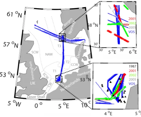
The North Sea (Fig. 1) is located on the north-western Euro-pean continental shelf. In the east and southeast it is bounded by the European continent, by the British Isles in the west and south, and by the Norwegian west coast in the northeast. The circulation is anti-cyclonic and the sea receives warm water from the North Atlantic Current (NAC) through the north-west openings and fresh water mainly from Baltic Sea outflow and European rivers.

Generally, the deeper northern and central parts are strati-fied during summer while much of the shallow south is per-manently mixed. Stratification in different areas can occur in salinity or (seasonally) in temperature. The VOS lines consistently cover six of the nine hydrographical regions and

Copernicus Publications

Bahnhofsallee 1e 37081 Göttingen Germany

Martin Rasmussen (Managing Director) Nadine Deisel (Head of Production/Promotion)

Contact

publications@copernicus.org http://publications.copernicus.org Phone +49-551-900339-50 Fax +49-551-900339-70

Legal Body

Copernicus Gesellschaft mbH Based in Göttingen Registered in HRB 131 298 County Court Göttingen Tax Office FA Göttingen USt-IdNr. DE216566440

Page 1/1

Fig. 1. Map of the North Sea, including the most persistent tracks

(blue) of the VOS ships (Nuka Arctica and Trans Carrier) during 2005–2007, names of water masses (as initials) and their corre-sponding hydrographic regions (dotted grey, after Lee, 1980). Solid rectangle (at the southern tip of Norway) indicates the area where the two VOS tracks crossover and from which data on Fig. 3 was acquired. Dashed rectangles indicate two sites at which the inter-annual variability is investigated using data from years and loca-tions shown on the insets where blue indicates VOS tracks; red, green, and grey denote underwayfCOsw₂ cruise tracks; black show stations. Water masses shown on the map are CCW: Continental Coastal Water; NAW: North Atlantic Water; SW: Skagerrak Water; SCW: Scottish Coastal Water; ECW: English Coastal Water; CW: Channel Water; T1–T3: transitional water 1–3.

their corresponding water masses as identified by Lee (1980) (Fig. 1). The Continental Coastal Water (CCW) flows along the European continent from Dover Strait to about 56◦_{N and}

2 Data and methods

2.1 VOS data and co-located parameters

Underway measurements offCOsw₂ and sea surface temper-ature (SST) were obtained aboard two containerships MS

Trans Carrier (operated by Seatrans AS, Norway www.

seatrans.no) and MV Nuka Arctica (Royal Arctic Lines of Denmark). The route of MS Trans Carrier has changed over time and today the ship crosses the North Sea along a tran-sect at roughly 5◦E (Fig. 1). At the start of the project, the ship track had a triangular shape as the ship also called on the port of Immingham (UK) in addition to Bergen (Norway) and Amsterdam (The Netherlands). For the present analyses, we use data exclusively from the line connecting Norway and The Netherlands, since it has been the most persistent track. Note that even within this transect the ship track can change slightly, for example, due to weather conditions. Moreover, north of 58.5◦N the ship frequently stopped at several small ports before Bergen. For consistency, data acquired within the geographic rectangle 53.2◦_N–58.5◦_{N and 4.4}◦_E–5.5◦_E

(henceforth the NS-transect) and during September 2005– December 2007 are used for the present analyses. Between February and December 2006, the VOS line was serviced by a sister ship MS Norcliff using the same measurement sys-tem.

The second ship, MV Nuka Arctica, crosses the North Sea approximately every three weeks along a transect (henceforth the WE-transect) between 59.5–57.7◦N heading southeast until 7◦E, and then continues east until 10◦E, where it turns south and enters the port of Alborg, Denmark. ThefCOsw₂ system was installed onboard during 2004, but the data anal-ysed here are from 2005 through 2007.

The measurement method used aboard MS Trans Carrier is identical to that used aboard MV Nuka Arctica, which was described in detail by Olsen et al. (2008). The instruments aboard the two ships are replicates and are a modified version of those described by Feely et al. (1998) and Wanninkhof and Thoning (1993). Briefly, for both ships, thefCOsw₂ instru-ment uses a non-dispersive infrared (NDIR) CO2/H2O gas analyzer (LI-COR 6262) to determine the CO2concentration in a headspace air in equilibrium with a continuous stream of seawater. Every 3 min an analysis is done and the instrument is calibrated roughly every six hours with three reference gases with approximate concentrations of 200 ppm, 350 ppm, and 430 ppm, which are traceable to reference standards pro-vided by National Oceanic and Atmospheric Administra-tion/Earth System Research Laboratory (NOAA/ESRL). The zero and span of the NDIR response are determined once a day using a CO2-free gas (N2)and the reference standard with highest CO2concentration, respectively.

The seawater temperature in the equilibrator (Teq) and SST (measured at a dedicated seawater intake 2–4 m below water level; 2 m in 2005 for M/S Nuka Arctica and 4 m for all other data) were also recorded along with the raw mole

frac-tion data (xCO2)from the NDIR. The temperature measure-ments were done using Hart Model 1521digital thermome-ters from Hart Scientific, Inc.

xCO2is converted to seawaterfCO2in two steps. First,

fCO2at the equilibrator temperature is computed according to (K¨ortzinger, 1999):

fCOeq₂ =xCOeq₂ (peq−pH2O)exp(p

eqB+2δ

RTeq ) (1)

wherepeqis equilibrator pressure,pH2Ois the vapour

pres-sure (Weiss and Price, 1980),R is the gas constant, andB

andδare the first and second cross virial coefficients (Weiss, 1974).

Next, the CO2 fugacity at in situ temperature (fCOsw₂ ) was computed by taking into account the difference between equilibration and in situ temperatures (SST-Teq<0.5◦C) ac-cording to (Takahshi et al., 1993):

fCOsw₂ =fCOeq₂exp[0.0423(SST−Teq)] (2) Data for sea surface salinity (SSS) and monthly mean sea-level pressure (MSLP) were co-located with the VOS data from gridded fields obtained from different publicly accessi-ble databases along the tracks of the ships. The SSS data are an ocean analyses product of the Met Office’s Forecasting Ocean Assimilation Model (Bell et al., 2006). The MSLP data were made available by Physical Science Division of NOAA/ERSL (http://www.cdc.noaa.gov/cdc/).

Monthly data for atmosphericxCO2were obtained from the NOAA/ESRL Global Monitoring Division (ftp://140. 172.192.211/ccg/co2/flask/month/) for the two stations Mace Head, Ireland (53.33◦N, 9.9◦W) and station Mike (66◦N, 2◦E) for the years 2005 to 2007. In order to account for the latitudinal dependency, the monthlyxCO2data have been fit-ted to linear functions of latitude. Hence, the atmospheric

xCO2value was determined for eachfCOsw₂ sample point. The resulting mole fractions were converted to atmospheric fugacity of CO2,fCOatm₂ , using Eq. (1) except that SST and MSLP were used instead ofTeqandpeq, respectively.

VOS data consistency and temporal coverage

1 2 3 4 5 6 7 8 9 101112

0

5000

10000

NS-transect

1 2 3 4 5 6 7 8 9 101112

0

2000

4000

WE-transect

Number of obser

va

tions

Month

2005 2006 2007

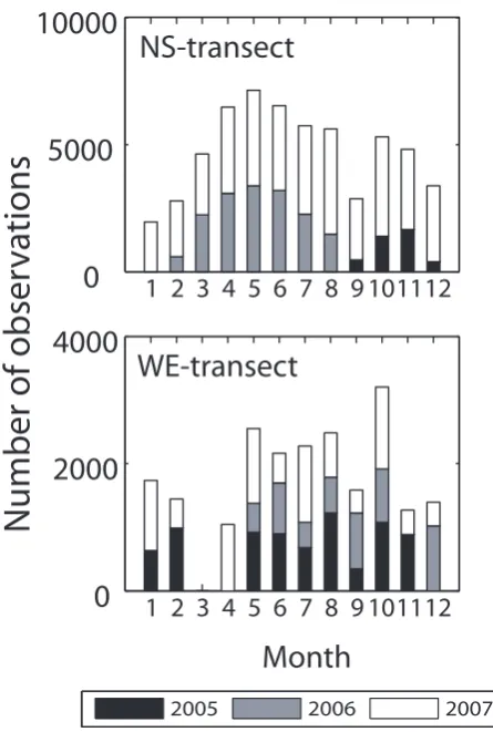
Fig. 2. Number offCOsw₂ observations per month made from 2005

to 2007 along the NS- and WE-transects. Note that only data used in this study is reported on the plot (other data were discarded due to various reasons detailed in Sect. 2).

have been organized into 0.27◦_E×0.38◦_{N×7 days bin}

av-erages for each year. Linear regressions between the aver-aged data (Fig. 3) resulted in residuals of 0±0.6◦C for SST and 1±13 µatm forfCOsw₂ meaning that there are no (or neg-ligible) systematic differences between data acquired by the two measurement systems. Moreover, the large standard de-viations of the residuals (±0.6◦C and±13 µatm) most prob-ably reflect the weekly and mesoscale spatial variability.

2.2 Cruise data

Data acquired by scientific cruises and those measured aboard VOS ships are often complementary in the sense that the latter contains high frequency measurements but is lim-ited in space and parameters while the former is limlim-ited in time but can be basin wide and normally contain a whole suit of parameters. In this work, we take advantage of this typical complementarity by augmenting the VOS data with subsets of data from ten cruises. Five of the cruises were conducted in the North Sea aboard RV Pelagia (18 August–

Fig. 3. A comparison offCOsw₂ (upper) and SST (lower) data

ac-quired from the NS- and WE-transects in the crossover area (57.94– 58.32◦N, 5.23–5.5◦E, see Fig. 1). Data from each transect have been organized into 0.27◦E×0.38◦N×7 days bin averages for each year in order to minimize differences due to spatial and/or temporal variations.

13 September 2001, 6–29 November 2001, 11 February–5 March 2002, 6–26 May 2002, and 17 August–6 September 2005). These data have been described in detail by others (Thomas et al., 2004, 2007; Bozec et al., 2005). Briefly, the RV Pelagia cruises covered the North Sea during all four seasons and obtained station data with a sampling resolution of 1◦ and underway data with one minute frequency sam-pling. During each cruise, water samples were collected for parameters including (but not limited to) dissolved inorganic carbon (DIC), total alkalinity (AT), salinity and temperature. The DIC concentrations were determined by the coulomet-ric method (e.g. Johnson et al., 1993) with a precision bet-ter than 1.5 µmol kg−1_{. UnderwaypCO}

4.5 6.5 8.5 10.5 12.5 14.5 16.5 18.5 6 8 10 12 14 14 16 18 8 La t (N) NS-transect 54 55 56 57 58 29 30 31 32 33 34 35 36 3132 33 33.8 33.8 33.8 34 34 34 34 La t (N) 54 55 56 57 58 210 235 260 285 310 335 360 385 410 435 260 285 310 310 335 335 360 360 335 385 385 360 410 285 360 435 360 La t (N) 54 55 56 57 58 -170 -120 -70 -20 20 70 -120 -95 -70 -70 -45 -45 -20 -20 -45 0 0 20 20 -20 45 -95 -45 0 -20 0 -20 0 La t (N)

1 2 3 4 5 6 7 8 9 10 11 12

54 55 56 57 58 6.5

8.5 10.5 14.5 12.5

16.5 Lon(E) WE-transect -2 0 2 4 6 8 10 30 31 32 32 33 33

33.8 34 ₃₄

35 35

30 33₃₂

Lon(E) -2 0 2 4 6 8 10 260285 310 310 310 335 335 360 285 285 360 Lon(E) -2 0 2 4 6 8 10 -95 _-70 -45 -45 -70 -45 -20 -95 -95 -20 0 -120 Lon(E)

1 2 3 4 5 6 7 8 9 10 11 12

-2 0 2 4 6 8 10 45 -45 0 -95 -145 95 0 A B C D E F G H

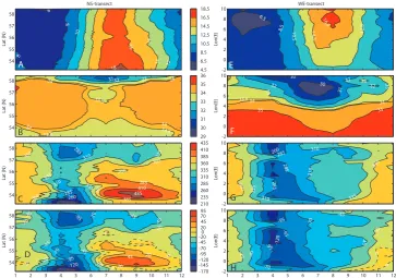
Fig. 4. Hovm¨oller diagrams of SST (A and E), SSS (B and F),fCOsw₂ (C and G), and1fCO2(D and H) along the NS-transect (left

column) and WE-transect (right column). For (D) and (H), note the change of contour intervals from 25 to 20 each sides of the 0 contour (dashed). The seasonal cycles shown in the figure are for a composite year consisting of the months depicted on Fig. 2 (above). For (G) and (H), the month March is filled by interpolation.

in one-minute intervals. The underwaypCO2data were con-verted tofCOsw₂ by subtracting 0.3% (Weiss, 1974).

Five earlier cruises were conducted in the coastal North Sea along the Netherlands in 1987 (9–12 March, 13–16 April, 13–14 July, 3–4 August, and 23–25 November). Cruises in March, April and November were carried out with the research ship “Aurelia” of the Netherlands Institute for Sea Research. The two summer cruises were made with the research vessel “Holland” of the Ministry of Water Manage-ment of the Netherlands. Samples were taken from 2 m depth for the determination ofATand DIC in addition to SST and SSS. DIC andATwere measured with a potentiometric titra-tion with strong acid (HCl) with a measurement precision of 0.3%. A more detailed description of the surveys and mea-surement methods can be found in Hoppema (1990, 1991).

The 1987 cruise data for DIC andAT were converted to

fCOsw₂ values using the constants of Mehrbach et al. (1973) refit by Dickson and Millero (1987) and simultaneously ac-quired data for seawater temperature, salinity, phosphate and silicate. For the few samples of which no nutrient data were available, silicate and phosphate were set to 0, a choice that has negligible effects on the results. The random uncertainty associated with the computedfCOsw₂ values was estimated to be±20 µatm. It was difficult to assess the systematic er-rors since the measurements were done before the availabil-ity of any Certified Reference Material and the data are from a highly variable coastal area.

3 Results and discussion

3.1 Seasonal and spatial variations

Figure 4 shows the seasonal and spatial variations of SST, SSS, fCOsw₂ , and 1fCO2 along the two transects in the North Sea for a composite year.

For the NS-transect, SST shows seasonal changes with an amplitude of over 11◦_{C being lowest during winter,}

increas-ing throughout sprincreas-ing, reachincreas-ing maximum durincreas-ing summer and decreasing throughout fall until reaching again minimum winter values (Fig. 4a). SST increases southwards along the transect (Fig. 4a), due to the solar radiation input which de-creases with latitude in the North Sea (Otto et al., 1990). Lin-ear regression between SST and latitude resulted in statisti-cally significant and negative slopes (Table 1) throughout the year. The magnitude of the gradient, however, is smallest during winter and strongest during fall (Table 1).

Table 1. Monthly distribution of latitudinal gradients infCOsw₂ and SST. Slopes (a, in µatm◦N−1or◦C◦N−1)and corresponding statistics obtained from linear regressions betweenfCOsw₂ or SST and latitude are shown. Positive values indicate properties increasing northwards and vice versa. ForfCOsw₂ the gradient was determined for two regions, 54.5–58.5◦N and 54.5–53.25◦N. For clarity, p-values are shown only where these are>0.05.

Month Annual

For: 1 2 3 4 5 6 7 8 9 10 11 12 mean

SST a −0.1 −0.1 −0.1 −0.3 −0.5 −0.3 −0.3 −0.3 −0.7 −0.7 −0.6 −0.3 −0.4

r 0.4 0.4 0.4 0.9 0.9 0.9 0.8 0.8 1 0.9 0.9 0.8 1.0

p

fCOsw₂ (54.5–58.5◦N) a −4 −4 −9 −6 −2 −11 −23 −27 −27 −23 −10 −4 −12

R 0.6 0.8 0.7 0.5 0 0.5 0.9 0.9 0.9 0.9 0.8 0.5 0.9

p 0.54

fCOsw

2 (54.5–53.25

◦_{N) a 13 14 81 106 41 29 80 55 66 43 24 23 48}

r 0.9 0.8 0.9 0.9 0.9 0.9 0.9 0.9 0.8 0.8 0.7 0.8 0.9

p

and most saline during winter and early spring, and with in-creasing/decreasing salinity throughout fall/spring.

The most remarkable feature in the seasonalfCOsw₂ cy-cle along the NS-transect (Fig. 4c) is the decrease during spring whenfCOsw₂ reaches values<320 µatm everywhere due to biological carbon uptake during the spring phyto-plankton bloom (Frankignoulle and Borges, 2001; Thomas et al., 2004). During the rest of the year, thermodynamic, rem-ineralization and mixing processes take over the control of

fCOsw₂ (the importance of the different controls forfCOsw₂ is discussed in Sect. 3.1.1) which shows values≥360 µatm, ex-cept for areas north of 56◦N where values<360 µatm persist until October. Apart from the southern end of the transect (south of 54◦N),fCOsw₂ increases southwards (Fig. 4c and Table 1) throughout the year although the gradient is statis-tically insignificant during May (Table 1). ThefCOsw₂ gra-dient is partly due to the above-mentioned SST gragra-dient (an-nual mean:−0.36◦_C◦_N−1_{, Table 1) which theoretically} ac-counts for about half of the observedfCOsw₂ gradient (an-nual mean: −12.4 µatm◦N−1, Table 1) becausefCOsw₂ in-creases by about 4% for every 1◦C increase in temperature (Takahashi et al., 1993). The rest of thefCOsw₂ gradient is probably due to the fact that in the shallow southern parts of the North Sea permanent mixing brings up remineralized carbon into the surface and elevatesfCOsw₂ , whereas in the central and northern parts stratification prevents remineral-ized carbon from reaching the surface (Thomas et al., 2004). This hypothesis draws support from the fact that the gradi-ent is strongest during summer and early fall (Table 1) when the majority of the organic matter formed during the pro-ductive season is remineralized. Approaching at the coast of the Netherlands (south of 54◦N), however, fCOsw₂ de-creases sharply southwards throughout the year (Fig. 4c and Table 1). Additionally, cruise data acquired along the NS-transect show that this region exhibits a surfaceAT-SSS lationship (Table 2) that is almost identical to the one

re-Table 2. Values of coefficients and statistical parameters

for two relationships between AT (µmol kg−1) and salinity (AT=a·salinity+b). The relationships were obtained by linear re-gressions using data acquired along the two transects (see Fig. 1) during four RV Pelagia cruises (in 2001 and 2002) and during the 1987 coastal cruises. Data from north of the 54◦N have been de-spiked by binning it into 0.5◦N×0.5◦E grid prior to regressions.

Parameter NS-transect WE-transect

a 13.3±3.2 −11.3±1.7 13.86±1.44

b 1835±110 2698±54 1817.46±48.02

Standard error

of the estimate ±9 ±28 ±6

r 0.75 0.74 0.95

p <0.001 <0.0001 <0.0001

Geographic limit 54–60◦N 52.5–54◦N 57.5–59◦N

ported for the German Bight (Brasse et al., 1999) where the surface seawater receives excess total alkalinity due to river runoff from the central European rivers (Kempe and Pegler, 1991) and water-sediment interaction (Brasse et al., 1999; Thomas et al., 2009). Therefore, excess total alka-linity from the above-mentioned processes conceivably re-sults in the relatively lowerfCOsw₂ in the southernmost part of the transect. Furthermore, a closer inspection of Fig. 4c reveals that the south is characterised by a strongerfCOsw₂ spring drawdown resulting in enhanced seasonal amplitude (≈230 µatm) compared to central (≈180 µatm) and northern regions (≈100 µatm).

The seasonal cycle of 1fCO2 (Fig. 4d) resembles that of fCOsw₂ (Fig. 4c) because the seasonal amplitude of

Table 3. Monthly distribution of longitudinal gradients infCOsw₂ and SST. Slopes (a, in µatm◦E−1or◦C◦E−1)and corresponding statistics obtained from linear regressions betweenfCOsw₂ or SST and longitude are shown. Positive values indicate properties increasing eastwards and vice versa. For clarity, p-values are shown only where these are>0.05.

Month Annual

For: 1 2 3 4 5 6 7 8 9 10 11 12 mean

SST a −0.1 −0.3 0 −0.1 0.1 0.3 0.3 0.4 0.3 0.1 0 −0.1 0.1

r 0.9 0.9 0 0.5 0.9 0.9 0.9 0.9 0.9 0.9 0 0.8 0.9

p 0.4

fCOsw₂ a −0.3 0.1 0 −4.1 1.2 2 1.6 −0.2 −1.3 −2.7 −3.4 −1.2 −0.8

r 0 0 0 0.5 0.3 0.6 0.5 0 0.3 0.6 0.9 0.5 0.5

p 0.3 0.8 0.2 0.6 0.2

CO2undersaturation (1fCO2≈−50–170 µatm) is observed during spring, while during summer and early fall, sur-face waters in the southern area become supersaturated (1fCO2>0). This seasonal cycle of 1fCO2 is in good agreement with the one reported by Thomas et al. (2004) who constructed seasonal averages offCOsw₂ based on data from four basin-wide cruises in the North Sea.

Data from the WE-transect (Fig. 4e–h) confirm the sea-sonal variations reported above for the northernmost part of the NS-transect. Additionally, this data subset enables us to compare east-to-west and north-to-south gradients for SST and fCOsw₂ . SST shows seasonal change with an ampli-tude of over 10◦_{C, being coldest in February and March and}

warmest in August (Fig. 4e). Furthermore, during winter and early spring, SST decreases eastwards (Table 3), but from late spring through fall the SST gradient reverses as a result of decreased mixed layer combined with solar radiation input that increase eastwards in the North Sea (Otto et al., 1990).

The spatial variations of SSS depict the water masses: the saline NAW (SSS>35) is usually encountered in the west-ern part of the transect (Fig. 4f), the fresh SW in the east. Also evident from Fig. 4f is the seasonality for SW, be-ing more fresh (SSS<31) during summer (July) and more saline (SSS>33) during winter (January). Additionally, the 35 isohaline retreats westwards during summer as also was reported by Lee (1980).

Values of fCOsw₂ are highest (360–380 µatm) during late fall and winter and lowest (≈260 µatm) during spring (Fig. 4g). Furthermore, the lowfCOsw₂ values during spring seem to appear first in the eastern side around April and prop-agate westwards. In the region west of the Prime Meridian, the lowestfCOsw₂ values occur in June. Conversely, the re-covery offCOsw₂ towards maximum winter values seems to start in the west around August and propagate eastwards. Apart from these two features,fCOsw₂ values do not show any systematic gradients along the WE-transect (Table 3). Nevertheless, a linear regression between annual fCOsw₂ data and longitude resulted in a statistically significant, but weak slope with poor statistics (Table 3, last column). The

most important feature in1fCO2(Fig. 4h) is that it is nega-tive everywhere along the transect, showing that the area is a year-round sink for atmospheric CO2.

The controls offCOsw₂

We decomposed the seasonal signal of fCOsw₂ data into individual components due to variations in SST, in air-sea CO2 exchange, in SSS, and in combined mixing and biol-ogy (a choice to be explained shortly), according to Olsen et al. (2008):

dobsfCOsw2 =dsstfCOsw2 +dasefCOsw2 +dsssfCOsw2

+dm&bfCOsw₂ (3)

where dobs fCOsw₂ is the observed monthly change in

fCOsw₂ ,dsstfCOsw₂ is the change due to SST changes,dase

fCOsw₂ is the change due to air-sea gas exchange, anddsss

fCOsw₂ anddm&bfCOsw₂ are the changes due to salinity vari-ations and mixing plus biology, respectively. Details on the computations of each term are given by Olsen et al. (2008). Here, we only mention that; (i) no nutrient data were ac-quired along the transects and, thus,dm&b fCOsw₂ is deter-mined as a residual i.e. as the monthly change in fCOsw₂ that is left unexplained by the other processes, (ii) The de-termination ofdsssfCOsw₂ requires the knowledge ofATin the surface seawater, whiledasefCOsw2 requires estimates of the air-sea CO2 flux (Fase). We used AT versus SSS rela-tionships observed along the NS- and WE-transects, based on data collected during the four RV Pelagia cruises con-ducted in 2001 and 2002. TheAT-SSS relationships and their statistics are given in Table 2. For the computation ofFase, we used 6-hourly wind speed data from NCEP/NCAR (Na-tional Centers for Environmental Prediction/The Na(Na-tional Center for Atmospheric Research). Gas transfer velocity was computed from wind speed using the relationship of Wan-ninkhof (1992).

-80 -40 0 40 A

NS-transect

-80 -40 0 40 B

-80 -40 0 40

M

on

thly fC

O

change (µa

tm)

C

-80 -40 0 40 D

2 4 6 8 10 12 -80

-40 0 40 E

F

2005/2006

G

H

I

2 4 6 8 10 12 J

K 2007

L

M

N

2 4 6 8 10 12 O

P

South of 55.5 N

Q

R

S

2 4 6 8 10 12 T

U

row 1: observed North of 57.5 (WE-transect)

V

row 2: dsstfCO2sw

W

row 3: d_asefCO₂sw

X

row 4: d_sssfCO₂sw

2 4 6 8 10 12 Y

row 5: d_m&bfCO₂sw

Month

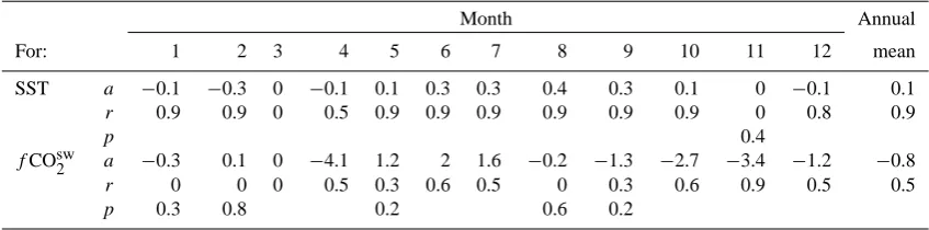
Fig. 5. Monthly changes infCOsw₂ as observed (first row) and expected due to: SST changes (second row), air-sea CO2exchange (third

row), SSS changes (fourth row) and biology plus mixing (last row). Negative values reflect a decrease infCOsw₂ and vice versa. The changes are shown for five cases: along the NS-transect (first column starting from left), for the period 2005/2006 (2nd column), for the year 2007 (3rd column), for the region south of 55.5◦N (4th column), and for the WE-transect (last column). The latter is referred to as north of the 57.5◦N in Sect. 3.1.1 of the main text.

periods 2005/2006 and 2007 (columns 2 and 3) and for the southern and northern regions of the North Sea (columns 4 and 5). Generally, the largest monthlyfCOsw₂ changes are observed from February to July. During this six month pe-riod,fCOsw₂ decreases during the first three months and in-creases during the last three (Fig. 5, row 1). During the rest of the year, both the magnitude and direction of monthly

fCOsw₂ change is highly dependent on the region and on the year. For instance, fCOsw₂ increases from August to November in the north (panel U), while during the same pe-riod,fCOsw₂ decreases in the south (panel P). Similarly, data from 2005/2006 show a markedfCOsw₂ decrease during Au-gust and September (panel F), whereas for the same period in 2007, a small increase was observed (panel K).

As to the importance of differentfCOsw₂ drivers, monthly

fCOsw₂ changes brought about by mixing and biology (row 5) dominate (−80 to 40 µatm month−1)together with SST-induced changes (row 2, −40 to 60 µatm month−1), whereas changes due toFase(row 3) are of intermediate im-portance (−10 to 35 µatm month−1)and changes from SSS (row 4) are negligible (<5 µatm month−1) (Fig. 5). Note that the changes from SSS are strongest on the WE-transect (≈10 µatm month−1_{), which is strongly influenced by SW,} the water mass with most significant seasonal variation in SSS (Fig. 4f).

The combination of the second, third and last rows of Fig. 5 suggests that the increasing effect of warming on

100 200 300 400 500

A

2 3 4 5 6 7 8 9 10 11 12 100

200 300 400 500

B

0 5 10 15 20 25

2 3 4 5 6 7 8 9 10 11 12 0

10 20 30

Month Month

2 3 4 5 6 7 8 9 10 11 12

1 1

1

2 3 4 5 6 7 8 9 10 11 12 1

fC

O2

(µa

tm)

fC

O2

a

t 12

oC (µa

tm)

SST (

oC)

Chla (mg m

-3) C

D

100 200 300 400 500

E

2 3 4 5 6 7 8 9 10 11 12 100

200 300 400 500

F

0 5 10 15 20 25

2 3 4 5 6 7 8 9 10 11 12 0

10 20 30

1

2 3 4 5 6 7 8 9 10 11 12 1

1

2 3 4 5 6 7 8 9 10 11 12 1

fC

O2

(µa

tm)

fC

O2

a

t 12

oC (µa

tm)

SST (

oC)

Chla (mg m

-3) G

H

VOS: 2007 2006 2005 Cruises: 2005 2002 2001 1987

Fig. 6. Seasonal cycles forfCOsw₂ (A and E), temperature normalizedfCOsw₂ (B and F), SST (C and G), and co-located SeaWiFS

Chlorophyll-a(D and H) for different years. All data were averaged weekly. For chl-a, only values between 0 and 30 mg m−3are considered realistic and plotted. Panels (A)–(D) show data acquired from a 1.0◦×1.0◦site on the northern North Sea (57.5–58.5◦N, 4.8–5.8◦E; see Fig. 1) for which underwayfCOsw₂ and SST data from 2001, 2002, and 2005–2007 are available. Panels E–H show data acquired from a 0.6◦×1.0◦site in the southern North Sea (52.5–53.1◦N, 3.6–4.6◦E; see Fig. 1) for which also station data from 1987 are available in addition to underway data from 2001, 2002, and 2005–2007.

The seasonal amplitudes offCOsw₂ due to the two most important drivers (changes in SST and biology plus mixing) can be estimated by integrating the monthly values ofdsst

fCOsw₂ and ofdm&bfCOsw2 , respectively. Peak-to-peak val-ues of the integrals give the magnitude of the seasonal am-plitudes and were computed from data shown on rows 2 and 5 of Fig. 5. For the NS-transect and using data from all years (panels B and E), we obtained seasonal amplitudes of 144 and−185 µatm due to changes of SST and biology plus mix-ing, respectively. However, the seasonal amplitudes due to changes of SST and biology plus mixing were respectively 195 and−169 µatm for 2005/2006, and 119 and−210 µatm for 2007. Thus, in the North Sea, the non-thermal control (bi-ology plus mixing) dominated if either the whole study pe-riod or the single year 2007 were considered. During 2006, however, the SST control dominated an inter-annual differ-ence that resulted from greater seasonal SST amplitude in 2006 (below, Fig. 6c and g).

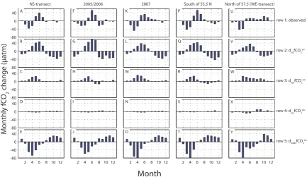
3.2 InterannualfCOsw₂ variations and trends

The interannual variability offCOsw₂ in the North Sea was investigated in two regions, which were chosen on the ba-sis of data availability (Fig. 1). The seasonal cycles for

fCOsw₂ , SST and co-located chlorophyll-a(chl-a)data from SeaWiFS (Sea-viewing Wide Field-of-view Sensor; http:// oceancolor.gsfc.nasa.gov) in the two regions from different years is depicted in Fig. 6. In both regions, the VOSfCOsw₂ shows substantial year-to-year variations especially during spring and summer when interannual differences (≈160– 200 µatm) are comparable to the seasonal changes (≈200– 250 µatm) (Fig. 6a and e). Fall and early winter show the smallest interannual fCOsw₂ variations, 10–50 µatm. Both seasonal and interannual variations appear to be somewhat larger in the southern site.

In order to comprehend the importance of the observed interannualfCOsw₂ changes for the air-sea CO2flux (Fase), we used a linear relationship between monthly1fCO2and

Fasevalues (y=−0.0035(±0.0003)·x;R=0.95;p <0.0001), which was identified during the evaluation of Eq. (3) (above). The difference in the annual mean1fCO2between 2005/2006 and 2007 is in the range of 15–25 µatm. Assum-ing this difference is representative for the whole NS-transect and using the aforementioned function, we estimated that ob-served fCOsw₂ changes have the potential to produce flux changes of 0.6–1.1 mol C m−2_yr−1_{, which is 50%–90% of} meanFasecomputed for the NS-transect using data from all years (1.2 mol C m−2_yr−1_{). However, interannualF}ase vari-ations in the North Sea are most probably substantially less than 90% because; (i) the southern region is characterised by enhanced seasonalfCOsw₂ changes (Fig. 6e–h) and, thus, it is likely that this location is more susceptible to nual changes than the rest of North Sea, and (ii) interan-nualfCOsw₂ variations can be accompanied by changes in wind speed with an opposing effect onFase. Indeed, when we computedFasefor the whole NS-transect using first data from 2005/2006 and then data from 2007, we obtained a year-to-yearFasevariation of 0.6 (=1.5–0.9) mol C m−2yr−1 i.e. 50% of the meanFase.

As to the cause of the observed interannual fCOsw₂ changes, several features of Fig. 6 deserve attention. Firstly, a comparison between the curves for the years 2006 and 2007 (Figs. 5e and 6a) reveals that the springtimefCOsw₂ draw-down by phytoplankton blooms starts some weeks earlier in 2007. Additionally, chl-a (Fig. 6d and h) indicate that the phytoplankton bloom in 2007 was stronger. In the southern region, mean chl-a concentration from March to April was 21±6 mg m−3 in 2007 and only 4.3±2.1 mg m−3 in 2006 (Fig. 6h). In the northern region, mean chl-a in late March was 13.7±1.5 mg m−3in 2007 and only 0.7±0.1 mg m−3in 2006 (Fig. 6d). Hence, the interannual variations in spring-timefCOsw₂ most probably result from changes in magnitude and timing of the spring phytoplankton bloom.

Secondly, interannual fCOsw₂ changes during summer can be partly accounted for by changes in SST. To ver-ify this, we normalized fCOsw₂ values to a constant SST (12◦C; Fig. 6b and f). A comparison between normal-ized fCOsw₂ for 2006 and 2007 reveals that SST changes account for the differences in fCOsw₂ in the northern re-gion during July and August (Fig. 6b). On the other hand,

fCOsw₂ differences between 2005 and 2007 observed in the northern region during July and August cannot be attributed to SST changes since the 2005 summertime fCOsw₂ re-mained at elevated values even after temperature normal-ization (Fig. 6b). These elevated summertimefCOsw₂ val-ues might be explained by changes in wind speed. High winds prevailed in the North Sea throughout 2005, with NCAR/NCEP wind speeds on average 2.4–2.7 m s−1higher than in 2006 and 2007. This would maintain enhanced car-bon flux from the atmosphere into the ocean during spring and, thus, could result in higher summertime fCOsw₂ val-ues. As to a third possible cause, AT variations were most probably not responsible for interannual summertime

fCOsw₂ variations in the northern site because the mean value of salinity normalized surface AT (AT35), computed from data acquired between 58.5◦N–54◦N during the RV

Pela-gia cruises, was 2301±5 µmol kg−1 and 2303±14 for

Au-gust/September 2001 and AuAu-gust/September 2005, respec-tively. This indicates that essentially allATvariations along this part of the NS-transect can be attributed to evapora-tion/dilution, a process which has equal effects onCTandAT and, thus, a negligible effect onfCOsw₂ . For the southern re-gion, the temperature normalization accounted for about half of thefCOsw₂ differences between 2006 and 2007 observed during August (Fig. 6f). Additionally,ATvariations resulting from changes of river runoff and/or sediment-water interac-tions might play a significant role in the interannualfCOsw₂ variations at this site. Thomas et al. (2009) reported that in the shallow southeastern North Sea, anaerobic degradation of organic matter releases total alkalinity which buffers the

fCOsw₂ increase from decaying phytoplankton blooms. It is likely that this alkalinity source varies between years due to the aforementioned variability in the biological productivity and, thus, produces some of the interannual fCOsw₂ varia-tions observed in the southern site.

year-to-year differences (±10 µatm, Fig. 6a) suggesting that only observations from these months may be appropriate for the determination of the trend. At present, there are too few data from these months for a robust analysis on this matter. For periods much longer than 20 years, however, using win-ter/fall data might be able to discern the long-term trend.

Kelley (1970) reported mean surface seawaterxCO2value of≈308±25 ppm in the North Sea. Kelley’s samples were taken early October 1967 at locations approximately on the 4◦E, most likely from the central North Sea as the ship sailed on the transatlantic route from Hamburg (Germany) to Boston (USA) which matched closely that of Buch (1939) (Kelley, 1970). Therefore, we converted the 1967 mean

xCO2 value tofCOsw₂ as described in Sect. 2.1, assuming equilibration pressure and temperature of 1 atmosphere and 14◦_{C. The result was subtracted from the meanfCO}sw

2 value measured between 55◦_N–57◦_{N on 1–15 October over the}

three years 2005, 2006, and 2007. We obtained anfCOsw₂ in-crease of 61±33 µatm (=364±22–303±24) for the 40 years elapsed since 1967. This implies that the surface water in central North Sea has tracked more or less the atmospheric CO2 increase (≈1.6 µatm yr−1 at Mauna Loa, Hawaii) in agreement with the fCOsw₂ growth rate recently reported for the North Atlantic (Takahashi et al., 2009). This find-ing is, however, somewhat surprisfind-ing since rapid and marked changes at decadal time-scales have been reported in the whole North Sea for SST (Edwards et al., 2002), phyto-plankton biomass (McQuatters-Gollop et al., 2007) and food-web structure (e.g. Beaugrand, 2004). Despite the above-mentioned physical and biological decadal changes, it seems that the influence of water inputs from the North Atlantic, whose waters track more or less closely the atmospheric CO2increase (e.g. Lef`evre et al., 2004), governs thefCOsw₂ growth rate in the central North Sea. Thus, the abovefCOsw₂ growth rate may be applicable in the northern North Sea as well since this region, too, receives large inputs of NAW. Conversely, the above estimatedfCOsw₂ growth rate prob-ably should not be extrapolated to the southern parts of the North Sea whereATchanges and eutrophication has stronger influence onfCOsw₂ (Thomas et al. 2009; Gypens et al., 2009).

Acknowledgements. This is a contribution to the EU IP

CAR-BOOCEAN (Contract no. 511176-2) and publication A243 of the Bjerknes Centre for Climate Research. The work of A. Omar has been supported by the Research Council of Norway (RCN). A.V.B. is a research associate at the F.R.S.-F.N.R.S. This work would not have been possible without the generosity and help of liner companies SeaTrans AS and Royal Arctic Lines, and the captains and crew of Trans Carrier and Nuka Arctica.

Edited by: W. M. Drennan

References

Beaugrand, G.: The North Sea regime shift: Evidence, causes, mechanism and consequences, Prog. Oceanogr., 60, 245–262, 2004.

Bell, M. J., Barciela, R., Hines, A., Martin, M., Sellar, A., and Storkey, D.: The Forecasting Ocean Assimilation Model (FOAM) system, in: Ocean Weather Forecasting, edited by: Chassignet, E. P. and Verron, J., Springer, The Netherlands, 397– 411, 2006.

Borges, A. V. and Frankignoulle, M.: Daily and seasonal variations of the partial pressure of CO2in surface seawater along the Bel-gian and southern Dutch coastal areas, J. Mar. Syst., 19, 251– 266, 1999.

Borges, A. V.: Do we have enough pieces of the jigsaw to integrate CO2fluxes in the Coastal Ocean?, Estuaries, 28(1), 3–27, 2005. Borges A. V. and Frankignoulle, M.: Distribution and air-water

ex-change of carbon dioxide in the Scheldt plume off the Belgian coast, Biogeochemistry, 59, 41–67, 2002.

Borges, A. V., Delille, B., and Frankignoulle, M.: Budget-ing sinks and sources of CO2 in the coastal ocean: Diver-sity of ecosystems counts, J. Geophys. Res., 32, L14601, doi:10.1029/2005GL023053, 2005.

Borges, A. V., Ruddick, K., Schiettecatte, L.-S., and Delille, B.: Net ecosystem production and carbon dioxide fluxes in the Scheldt estuarine plume, BMC Ecology, 8(15), doi:10.1186/1472-6785-8-15, 2008.

Bozec, Y., Thomas, H., Elkalay, K., and De Baar, H.: The con-tinental shelf pump in the North Sea - evidence from summer observations, Mar. Chem., 93, 131–147, 2005.

Bozec, Y., Thomas, H., Schiettecatte, L.-S., Borges, A. V., Elkalay, K., and De Baar, H. J. W.: Assessment of the processes control-ling the seasonal variations of dissolved inorganic carbon in the North Sea, Limnol. Oceanogr., 51, 2746–2762, 2006.

Brasse, S., Reimer, A., Seifert, R., and Michaelis, W.: The influence of intertidal mudflats on the dissolved inorganic carbon and total alkalinity distribution in the German Bight, southeastern North Sea, J. Sea Res., 42, 93–103, 1999.

Buch, K.: Beobachtungen ¨uber das Kohlens¨aurengleichgewicht und ¨uber den Kohlens¨aureaustausch zwischen Atmosphare und Meer im Nordatlantichen Ozean, Acta Acad. Aboensis, Math. Phys., 11(9), 3–32, 1939.

Cai, W.-J., Dai, M. H., and Wang, Y. C.: Air-sea exchange of carbon dioxide in ocean margins: A province-based synthesis, Geophys. Res. Lett., 33, L12603, doi:10.1029/2006GL026219, 2006. Canadell, J. G., Le Qu´er´e, C., Raupach, M. R., Field, C. B.,

Buiten-huis, E. T., Ciais, P., Conway, T. J., Gillett, N. P., Houghton, R. A., and Marland, G.: Contributions to accelerating atmospheric CO2growth from economic activity, carbon intensity, and effi-ciency of natural sinks, P. Natl. Acad. Sci. USA, 104, 18353– 18354, 2007.

Chen, C. T. A. and Borges, A. V.: Reconciling opposing views on carbon cycling in the coastal ocean: continental shelves as sinks and near-shore ecosystems as sources of atmospheric CO2, Deep-Sea Res. II, 56, 578–590, 2009.

Dickson, A. G. and Millero, F. J.: A comparison of the equilibrium constants for the dissociation of carbonic acid in seawater media, Deep-Sea Res., 34, 1733–1743, 1987.

Sea, Mar. Ecol. Prog. Ser., 239, 1–10, 2002.

Feely, R. A., Wanninkhof, R., Milburn, H. B., Cosca, C. E., Stapp, M., and Murphy, P. P.: A new automated underway system for making high precisionpCO2 measurements onboard research ships, Anal. Chim. Acta, 377, 185–191, 1998.

Frankignoulle M. and Borges, A. V.: The European continental shelf as a significant sink for atmospheric carbon dioxide, Global Biogeochem. Cy., 15, 569–576, 2001.

Grasshoff, K., Ehrhardt, M., and Kremling, K. (eds.): Methods of Seawater Analysis (2nd ed.), Verlag Chemie, Weinheim, 1983. Gypens, N., Borges, A. V., and Lancelot, C.: Effect of

eutrophica-tion on air-sea CO₂fluxes in the coastal Southern North Sea: A model study of the past 50 years, Glob. Change Biol., 15, 1040– 1056, 2009.

Johnson, K. M., Wills, K. D., Butler, D. B., Johnson, W. K., and Wong, C. S.: Coulometric total carbon dioxide analysis for ma-rine studies: maximizing the performance of an automated gas extraction system and coulometric detector, Mar. Chem., 44, 167–187, 1993.

Hoppema, J. M. J.: The distribution and seasonal variation of alka-linity in the Southern Bight of the North Sea and in the western Wadden Sea, Neth. J. Sea Res., 26, 11–23, 1990.

Hoppema, J. M. J.: The seasonal behaviour of carbon dioxide and oxygen in the coastal North Sea along the Netherlands, Neth. J. Sea Res., 28, 167–179, 1991.

Lee, A. J.: North Sea: Physical Oceanography, in: The North-west European shelf Seas the seabed and the sea in motion II. Physical and Chemical Oceanography, edited by: Banner, F. T., Collins, M. B., and Massie, K. S., Elsevier Oceanography Series, 24B, Elsevier, Amsterdam, 467–493, 1980.

Lef`evre, N., Watson, A. J., Olsen, A., R´ıos, A. F., P´erez, F. F., and Johannessen, T.: A decrease in the sink for atmospheric CO2 in the North Atlantic, Geophys. Res. Lett., 31, L07306, doi:10.1029/2003GL018957, 2004.

Kelley, J. J.: Carbon dioxide in the surface waters of the North At-lantic ocean and the Barents and Kara seas, Limnol. Oceanogr., 15, 80–87, 1970.

Kempe, S. and Pegler, K.: Sinks and sources of CO2in coastal seas: the North Sea, Tellus, 43B, 224–235, 1991.

K¨ortzinger, A.: Determination of carbon dioxide partial pres-sure (pCO2), in: Methods of Seawater Analysis, edited by: Grasshoff, K., Kremling, K., and Ehrhardt M., 3rd ed., Wiley-VCH, Weinheim, 149–158, 1999.

K¨ortzinger, A., Thomas, H., Schneider, B., Gronau, N., Mintrop, L., and Duinker, J. C.: At-sea intercomparison of two newly designed underwaypCO2systems – encouraging results, Mar. Chem., 52, 133–145, 1996.

McQuatters-Gollop A., Raitsos, D. E., Edwards, M., Pradhan, Y., Mee, L. D., Lavender, S. J., and Attrill, M. J.: A long-term chlorophyll dataset reveals regime shift in North Sea phytoplank-ton biomass unconnected to nutrient levels, Limnol. Oceanogr., 52, 635–648, 2007.

Mehrbach, C., Culberson, C. H., Hawley, E. J., and Pytkowicz, R. M.: Measurements of the apparent dissociation constants of carbonic acid in seawater at atmospheric pressure, Limnol. Oceanogr., 18, 897–907, 1973.

Olsen, A., Brown, K. R., Chierici, M., Johannessen, T., and Neill, C.: Sea-surface CO₂ fugacity in the subpolar North Atlantic, Biogeosciences, 5, 535–547, 2008,

http://www.biogeosciences.net/5/535/2008/.

Otto, L., Zimmerman, J. T. F., Furnes, K., Mork, M., Saetre, R., and Becker, G.: Review of the physical oceanography of the North Sea, Neth. J. Sea Res., 26, 161–238, 1990.

Sabine, C. L., Feely, R. A., Key, R. M., Lee, K., Bullister, J. L., Wanninkhof, R., Wong, C. S., Wallace, D. W. R., Tilbrook, B., Millero, F. J., Peng, T.-H., Kozyr, A., Ono, T., and Rios, A. F.: The oceanic sink for anthropogenic CO2, Science, 305, 367–371, 2004.

Schiettecatte, L., Gazeau, F., Van der Zee, C., Brion, N., and Borges, A. V.: Time series of the partial pressure of carbon dioxide (2001–2004) and preliminary inorganic carbon budget in the Scheldt plume (Belgian coastal waters), Geochem. Geophy. Geosy., 7, Q06009, doi:10.1029/2005GC001161, 2006. Schiettecatte, L.-S., Thomas, H., Bozec, Y., and Borges, A. V.: High

temporal coverage of carbon dioxide measurements in the South-ern Bight of the North Sea, Mar. Chem., 106, 161–173, 2007. Takahashi, T., Olafsson, J., Goddard, J. G., Chipman, D. W., and

Sutherland, S. C.: Seasonal variation of CO₂and nutrients in the high-latitude surface oceans: a comparative study, Global Bio-geochem. Cy., 7, 843–878, 1993.

Takahashi, T., Sutherland, S. C., Sweeney, C., Poisson, A., Metzl, N., Tilbrook, B., Bates, N. R., Wanninkhof, R., Feely, R. A., Sabine, C. L., Olafsson, J., and Nojiri, Y.: Global sea-air CO2 flux based on climatological surface oceanpCO2, and seasonal biological and temperature effects, Deep-Sea Res. II, 49, 1601– 1622, 2002.

Takahashi, T., Sutherland, S. C., Wanninkhof, R., Sweeney, C., Feely, R. A., Chipman, D. W., Hales, B., Friederich, G., Chavez, F., Sabine, C., Watson, A., Bakker, D. C. E., Schuster, U., Metzl, N., Yoshikawa-Inoue, H., Ishii, M., Midorikawa, T., Nojiri, Y., K¨ortzinger, A., Steinhoff, T., Hoppema, M., Olafsson, J., Arnar-son, T. S., Tilbrook, B., Johannessen, T., Olsen, A., Bellerby, R., Wong , C. S., Delille, B., Bates, N. R., and De Baar, H. J. W.: Climatological mean and decadal change in surface oceanpCO₂, and net sea-air CO2flux over the global oceans, Deep-Sea Res. II, 554–577, 2009.

Thomas, H., Bozec, Y., Elkalay, K., de Baar, H. J. W., Borges, A. V., and Schiettecatte, L.-S.: Controls of the surface water partial pressure of CO2in the North Sea, Biogeosciences, 2, 323–334, 2005,

http://www.biogeosciences.net/2/323/2005/.

Thomas, H., Bozec, Y., Elkalay, K., and De Baar, H.: Enhanced open ocean storage of CO₂ from shelf sea pumping, Science, 304, 1005–1008, 2004.

Thomas, H., Prowe, A. E. F, Van Heuven, S., Bozec, Y., De Baar, H. J. W, Schiettecatte, L.-S., Suykens, K., Kon´e, M., Borges, A. V., Lima, I. D., and Doney, S. C.: Rapid decline of the CO2buffering capacity in the North Sea and implications for the North Atlantic Ocean, Global Biogechem. Cy., 21, GB4001, doi:10.1029/2006GB002825, 2007.

Thomas, H., Schiettecatte, L.-S., Suykens, K., Kon´e, Y. J. M., Shad-wick, E. H., Prowe, A. E. F., Bozec, Y., de Baar, H. J. W., and Borges, A. V.: Enhanced ocean carbon storage from anaerobic al-kalinity generation in coastal sediments, Biogeosciences, 6, 267– 274, 2009,

http://www.biogeosciences.net/6/267/2009/.

51B, 701–712, 1999.

Wanninkhof, R. and Thoning, K.: Measurement of fugacity of CO2 in surface water using continuous and discrete sampling meth-ods, Mar. Chem., 44, 189–201, 1993.

Wanninkhof, R.: Relationship between wind speed and gas ex-change over the ocean, J. Geophys. Res., 97, 7373–7382, 1992. Weiss, R. and Price, B. A.: Nitrous oxide solubility in water and

seawater, Mar. Chem., 8, 347–359, 1980.

Weiss, R. F.: Carbon dioxide in water and seawater: the solubility of a non-ideal gas, Mar. Chem., 2, 203–215, 1974.