Modeling of the circulation in the Northwestern Mediterranean Sea with the Princeton Ocean Model

(1)

www.ocean-sci.net/3/77/2007/

Ocean Science

Modeling of the circulation in the Northwestern Mediterranean Sea

with the Princeton Ocean Model

M. A. Ahumada1and A. Cruzado2

1_{Instituto de Recursos, Universidad del Mar, Puerto Angel, Oaxaca, M´exico} 2_{Centre d’Estudis Avanc¸ats de Blanes, CSIC, Blanes, Catalonia, Spain} Received: 4 April 2006 – Published in Ocean Sci. Discuss.: 9 August 2006

Revised: 14 November 2006 – Accepted: 2 February 2007 – Published: 9 February 2007

Abstract. The Princeton Ocean Model – POM (Blumberg

and Mellor, 1987) has been implemented in the Northwestern Mediterranean nested (in one-way off-line mode) to a gen-eral circulation model of the Mediterranean Sea – OGCM (Pinardi and Masetti, 2000; Demirov and Pinardi, 2002) in order to investigate if this model configuration is capa-ble of reproducing the major features of the circulation as known from observations and to improve what has been made by previous numerical modeling works. According to the model results, the large-scale cyclonic circulation in the northern part of the Northwestern Mediterranean is, at least in the upper layers, less coherent in winter and spring than in summer and autumn. Furthermore, there is evidence that the mesoscale structure (eddies and meanders) is, during all year, a significant dynamic characteristic in this region of the Mediterranean Sea. Finally, concerning the circulation in the lower layers, the model results have confirmed that Levantine Intermediate Water (LIW) and Western Mediterranean Deep Water (WMDW) follow essentially a cyclonic path during all year.

1 Introduction

The Mediterranean Sea is a semi-enclosed sea acting like an ocean system in which several temporal and spatial scales (basin, subbasin, and mesoscale) interact to form a highly complex and variable circulation (Fern´andez et al., 2005). Millot (1991) has mentioned that the major surface currents flowing along slope, can be affected by instability processes that sometimes lead to the generation of turbulent phenom-ena such as mesoscale eddies, which can induce relatively intense currents and great heterogeneity of the hydrological characteristics. On the other hand, Send et al. (1999) sustain

Correspondence to: A. Cruzado

(cruzado@ceab.csic.es)

that the development of an upper mixed layer by summer solar heating and the convective processes caused by win-ter cooling and strong winds produce seasonal changes in the near-surface circulation whose effects mainly consist of modulations in the intensity and smaller scale variability of the current systems. More recently, Molcard et al. (2002) have suggested that the main permanent features of the gen-eral circulation (Gulf of Lions cyclonic gyre, Rhodes cy-clonic gyre, Gulf of Syrte anticycy-clonic gyre) are induced by the permanent wind stress curl structure. They point out that the magnitude and spatial variability of the wind is impor-tant in determining the appearance or disappearance of some gyres such as the Tyrrhenian anticyclonic gyre and the Ionian cyclonic gyre. Concerning the circulation at deeper layers, it is generally accepted that it follows the topography of the different subbasins (La Violette, 1990), describing basically a cyclonic path.

(2)

0 1 2 3 4 5 6 7 8 9 10 39

40 41 42 43 44

Longitude (deg. E)

Latitu

d

e

(d

e

g

.

N

)

Depth (m)

0 200 500 700 1000 1500 2000 2500 2795 Italy France

Spain

Ligurian Sea

Catalan Sea

Gulf of Lions

Corsica

Sardinia Minorca

Majorca

Ibiza

T y r r h e n i a n

S e a

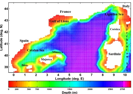
Fig. 1 The Northwestern Mediterranean Sea Model Domain and Bottom Topography based on the U.S. Navy Digital Bathymetric Data Base 5.

Fig. 1. The Northwestern Mediterranean Sea Model Domain and Bottom Topography based on the U.S. Navy Digital Bathymetric Data Base 5.

the Mediterranean Sea circulation, in some way, suggest that no single model is going to be the best one for all applica-tions. In this context, the state of the art continuously offers new perspectives with room for improvements of model de-sign, formulations, parameterizations, etc. In this work, a numerical modeling system based on the Princeton Ocean Model (Blumberg and Mellor, 1987) has been implemented in the Northwestern Mediterranean nested (in one-way off-line mode) to a general circulation model of the Mediter-ranean Sea – OGCM (Pinardi and Masetti, 2000; Demirov and Pinardi, 2002) in order to investigate if this model con-figuration is capable of reproducing the major features of the circulation as known from observations and to improve what has been made by previous numerical modeling works.

This article is organized as follows. A brief description of the principal characteristics of the Princeton Ocean Model, along with details of its configuration for the Northwestern Mediterranean Sea is given in Sect. 2. Atmospheric forcing and initial conditions used for the climatological integration of this model configuration are briefly analyzed in Sect. 3. The model results and discussions are presented in Sect. 4, and conclusions are offered in Sect. 5.

2 Numerical model

2.1 Model description

The Princeton Ocean Model (POM) is a 3-D primitive equa-tions ocean circulation model, which has been described in detail by Blumberg and Mellor (1987) and Mellor (2004). POM is a free surface, sigma coordinate model that uses a time-splitting technique to solve depth-integrated and fully three-dimensional equations with different time steps. The surface elevation, velocity, temperature, and salinity fields are prognosticated assuming the fundamental hypotheses: i)

Fig. 2 Spatial distribution of Net Heat Flux from ECMWF 1979-1993 reanalysis data: February (upper panel) and August (lower panel). Units are W/m2_.

15

Fig. 2. Spatial distribution of Net Heat Flux from ECMWF 1979– 1993 reanalysis data: February (upper panel) and August (lower panel). Units are W/m2.

that the seawater is incompressible, ii) that the pressure in any point of the ocean is equal to the weight of the column of water over it (hydrostatic approximation), and iii) that the density can be expressed in terms of a mean value and a small fluctuation (Boussinesq’s approximation). Consequently, in a system of orthogonal Cartesian coordinates, the governing equations are

∂Ui

∂xi

=0 (1)

∂(U,V )

∂t +

∂[Ui(U,V )]

∂xi +f (−V , U )=

−ρ₀−1h∂p_∂x,∂p_∂yi+∂

KM∂(U,V )∂z

∂z

+(FU, FV)

(2)

∂p

∂z = −ρg (3)

∂θ

∂t +

∂(Uiθ )

∂xi =

∂

KH∂θ∂z

∂z

+Fθ+∂R_∂z

(4)

∂S

∂t +

∂ (UiS)

∂xi

=

∂

KH∂S_∂z

(3)

Fig. 3 Spatial distribution of Wind Stress from ECMWF 1979-1993 reanalysis data: February (upper panel) and August (lower panel). Units are m2_/s2_.

16

Fig. 3. Spatial distribution of Wind Stress from ECMWF 1979-1993 reanalysis data: February (upper panel) and August (lower panel). Units are m2/s2.

Vertical mixing coefficients,KM andKH, are computed

ac-cording to the Mellor-Yamada 2.5 turbulence closure scheme (Mellor and Yamada, 1982). This scheme requires prognos-tic calculations of (q2)and (q2`), where the turbulent kinetic energy isq2

2 and the turbulence macro scale is (`). The equations that calculateq2andq2`are similar to those used for temperature and salinity and include production and dis-sipation source/sink terms. Horizontal diffusion terms (FU,

FV,Fθ, andFS)are computed using the Smagorinsky (1963)

formulation, implemented into POM according to Mellor and Blumberg (1986). The last term in Eq. (4), is the solar ra-diation flux that penetrates the sea surface. The UNESCO equation of state, as adapted by Mellor (1991) is used. The in situ density is determined as a function of salinity, poten-tial temperature and pressure; the latter being approximated by the hydrostatic relation and constant density.

2.2 Model configuration

The model domain comprises the northwestern region of the Mediterranean Sea, from 38.5◦N to 44.5◦N and from 0.5◦W to 10.5◦E. The bottom topography is based on the U.S. Navy Digital Bathymetric Data Base 5 (1/12◦×1/12◦)

mapped onto the model domain using bilinear interpolation.

Table 1. Model Parameters used during the Climatological Experi-ment.

Parameter Description Value

C Non-dimensional constant used in calculating 0.2

the horizontal viscosity for momentum

tprni Inverse horizontal Prandtl number 0.2

µM Background viscosity 0.00002

Z0 Bottom roughness length 0.01

1text External mode time step 9 s

1tint Internal mode time step 720 s

The resulting topography is shown in Fig. 1, which displays the major features of the domain including Sardinia, Corsica, Minorca, Majorca, and Ibiza Islands. In this model version (afterwards, NMS model) there are two open lateral bound-aries; at 38.5◦N and at 10.5◦E. The NMS model has been configured with a horizontal resolution of 1/16◦in latitude by 1/16◦in longitude, therefore with this resolution, the Rossby radius of deformation (10–20 km in the Mediterranean) is re-solved, and consequently, the NMS model configuration is adequate to simulate mesoscale structures (Fern´andez et al., 2005). In the vertical, the grid has 27 sigma layers with log-arithmic distributions at the surface and at the bottom and a linear distribution in between. Nine reduced thickness sigma layers have been laid at the surface while at the bottom there are six. Other significant model parameters are given in Ta-ble 1.

2.2.1 Open lateral boundary conditions

Along the two open lateral boundaries, the NMS model is forced with velocity, salinity and temperature fields obtained from the 8th year of the Mediterranean Sea OGCM climato-logical integration (perpetual year run). This Mediterranean Sea model is based on the rigid lid Modular Ocean Model (MOM), which was configured with a horizontal resolution of 1/8◦×1/8◦and 31 vertical levels and it was forced by the same atmospheric data set used here. For more details about the model configuration see Demirov and Pinardi (2002), Ko-rres and Lascaratos (2003) and Tonani (2003). Given that the NMS model has not the same horizontal resolution than the OGCM, a horizontal bilinear interpolation of the OGCM fields was necessary. Besides, as the vertical coordinate sys-tem is different, these data were transformed from z-levels to sigma coordinates using a linear interpolation. Finally, to avoid temporal discontinuities on the open lateral boundaries of the NMS model, all data are specified at each time step us-ing a linear interpolation in time between consecutive 10-day averaged fields.

(4)

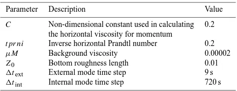
Fig. 4 Spatial distribution of Evaporation rate (E) from ECMWF 1979-1993 reanalysis data minus Precipitation (P) from Legates and Willmot (1991) monthly climatology: February (upper panel) and August (lower panel). Units are mm/month.

17 Fig. 4. Spatial distribution of Evaporation rate (E) from ECMWF 1979–1993 reanalysis data minus Precipitation (P) from Legates and Willmot (1991) monthly climatology: February (upper panel) and August (lower panel). Units are mm/month.

described in detail by Zavatarelli et al. (2002), Korres and Lascaratos (2003), and Zavatarelli and Pinardi (2003). On the other hand, after several sensitivity tests to different for-mulations for the open lateral boundary conditions, the NMS model solution did not show overly sensitive to the velocity component tangential to the open lateral boundaries. For this reason, in this particular experiment, we set it to zero. For salinity and temperature, whenever the normal velocity is di-rected outwards from the NMS model’s domain (outflows), the values are extrapolated from the interior solution using an upstream advection scheme. Otherwise, in cases of in-flow through the boundary, salinity and temperature are pre-scribed from the OGCM outputs.

For the external mode, it is imposed ¯

U ,V¯=

H

(H+η) _¯

UOGCM,V¯OGCM

(6)

where U¯and V¯ are the vertically integrated velocities on the NMS model’s open lateral boundaries,H is the bottom depth,ηis the free-surface elevation, andU¯OGCMandV¯OGCM are the vertically integrated velocities from the OGCM out-puts. The ratioH(H+η)is employed to ensure the vol-ume continuity (Korres and Lascaratos, 2003; Zavatarelli et

Fig. 5 Sea Surface Temperature (SST) from MED6 monthly climatology: February (upper panel) and August (lower panel). The contour interval is 0.5ºC.

18

Fig. 5. Sea Surface Temperature (SST) from MED6 monthly cli-matology: February (upper panel) and August (lower panel). The contour interval is 0.5◦C.

al., 2002, 2003). Finally, tangential velocities were set to zero and a zero-gradient condition for the free-surface eleva-tion was used.

2.2.2 Surface boundary conditions

All atmospheric forcing (wind stress, heat flux and freshwa-ter flux components) are mapped onto the NMS model grid using bilinear interpolation. Additionally, during the model integration, the atmospheric forcing is specified at each ex-ternal or inex-ternal time step, using linear interpolation in time between successive fields. So, the surface boundary condi-tion for momentum is prescribed according to

KM

D (

∂ (u, v)

∂σ )= −ρ

−1 0 τx, τy

(7) where τx and τy represent the surface wind stress

com-ponents obtained from the European Center for Medium-Range Weather Forecasts (ECMWF) 1979–1993, 6-h reanal-ysis data on a regular 1◦by 1◦grid (for more details about these data, see Korres and Lascaratos, 2003) andρ0 is the density of reference taken as 1025 kg m−3(Mellor, 2004).

For temperature the following formulation is used

KH

D (

∂θ

∂σ)=

QT

ρ0Cp

+ C1

ρ0Cp(SST −T )

(5)

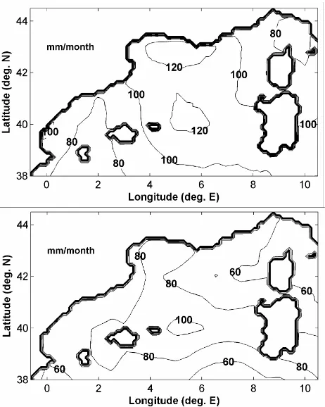
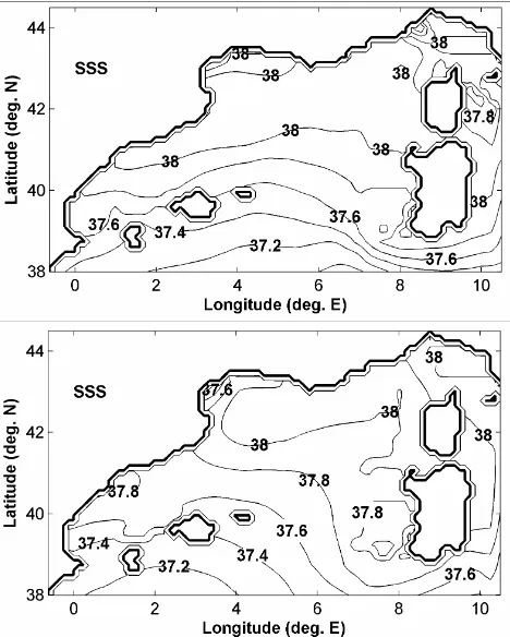
Fig. 6 Sea Surface Salinity (SSS) from MED6 monthly climatology: February (upper panel) and August (lower panel). The contour interval is 0.2.

19

Fig. 6. Sea Surface Salinity (SSS) from MED6 monthly climatol-ogy: February (upper panel) and August (lower panel). The contour interval is 0.2.

where QT represents the total heat flux and Cp the

spe-cific heat of seawater, 3986 Jkg−1 (Mellor, 2004). The second term in Eq. (8) is the heat flux correction term, whereSST is the sea surface temperature obtained from the MED6 monthly climatology,T is the temperature at the first layer of the NMS model, andC1 is a coefficient taken as 15 Wm−2◦C−1. In this way the heat flux is forced to produce a sea surface temperature consistent with the MED6 monthly climatology (Sorgente et al., 2003).

For salinity the surface boundary condition is given ac-cording to

KH

D (

∂S

∂σ)=

_E₋_P

ρ0

+C2(SSS−S) (9)

whereEcorresponds to the monthly evaporation rate calcu-lated according toE=QELV(Zavatarelli and Mellor, 1995;

Korres and Lascaratos, 2003; Sorgente et al., 2003), P is the monthly precipitation obtained from Legates and Willmot (1991). The second term in Eq. (9) is the freshwater flux cor-rection term, whereSSSis the sea surface salinity obtained from the MED6 monthly climatology,Sis the salinity at the first layer of the NMS model, andC2is a coefficient taken as 0.7 m/day. The correction term accounts for the imperfect knowledge ofE−P, especially ofP (Sorgente et al., 2003).

0 1 2 3 4 5 6 7 8 9 10

39 40 41 42 43 44

Latitu

d

e

(d

e

g

.

N

)

Depth = -5 m

1m/s

Salinity

36 36.5 37 37.5 38 38.5 39

0 1 2 3 4 5 6 7 8 9 10

39 40 41 42 43 44

Latitu

d

e

(d

e

g

.

N

)

Depth = -100 m

1m/s

Salinity

36 36.5 37 37.5 38 38.5 39

Fig. 7 Initial Conditions for velocity and salinity: at 5-m depth (upper panel) and at 100-m depth (lower panel), fromDecember of the 8th

year of the Mediterranean Sea OGCM climatological integration(source data: Mediterranean Forecasting System, 2002).

20

Fig. 7. Initial Conditions for velocity and salinity: at 5-m depth (upper panel) and at 100-m depth (lower panel), from December of the 8th year of the Mediterranean Sea OGCM climatological inte-gration (source data: Mediterranean Forecasting System, 2002).

Finally, where the Rhone and the Ebro rivers discharge their waters an additional term is included in the surface bound-ary condition for salinity so that the first term on the right side of Eq. (9) is considered as(E−P −Ri)/ρ0, where Ri

represents the river runoffs in ms−1.

Finally, for the turbulence kinetic energy and the turbu-lence master length scale, the surface boundary condition is prescribed according to Mellor (2004).

2.2.3 Bottom boundary conditions

(6)

0 1 2 3 4 5 6 7 8 9 10 39

40 41 42 43 44

Latitu

d

e

(d

e

g

.

N

)

Depth = -400 m

1m/s

Salinity

36 36.5 37 37.5 38 38.5 39

0 1 2 3 4 5 6 7 8 9 10

39 40 41 42 43 44

Latitu

d

e

(d

e

g

.

N

)

Depth = -1000 m

1m/s

Salinity

36 36.5 37 37.5 38 38.5 39

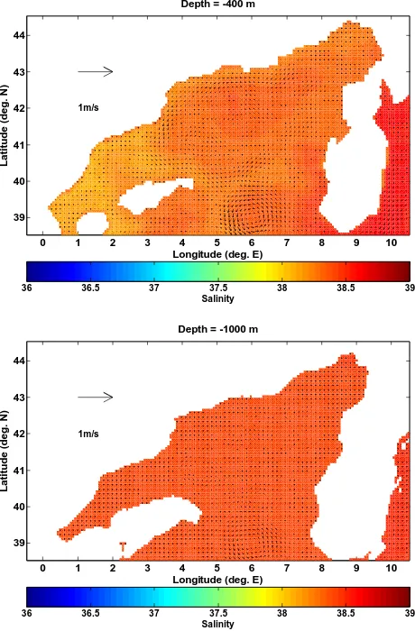
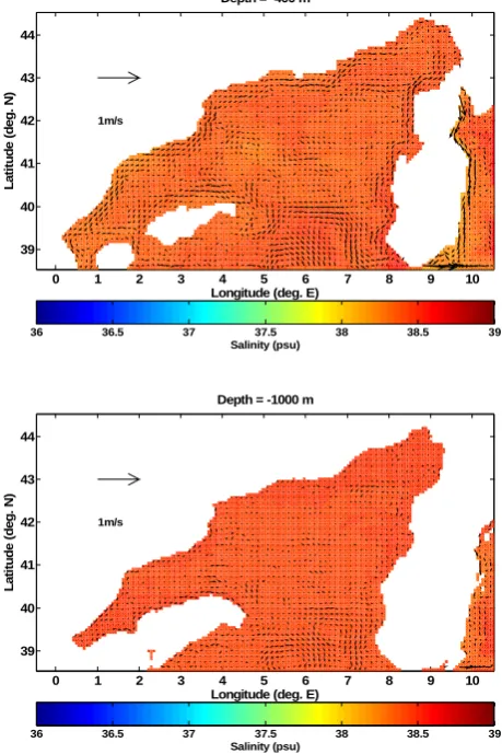
Fig. 8 Initial Conditions for velocity and salinity: at 400-m depth (upper panel) and at 1000-m depth (lower panel), from December of the 8th_{year of the Mediterranean Sea OGCM}

climatological integration (source data: Mediterranean Forecasting System, 2002).

21

Fig. 8. Initial Conditions for velocity and salinity: at 400-m depth (upper panel) and at 1000-m depth (lower panel), from December of the 8th year of the Mediterranean Sea OGCM climatological in-tegration (source data: Mediterranean Forecasting System, 2002).

3 Model forcing and initial conditions

3.1 Model forcing

3.1.1 Heat fluxes

The spatial distribution of the net heat flux in the NMS model’s domain for a typical winter (February) and summer (August) month is shown in Fig. 2. During February heat is lost throughout the domain, especially over the Gulf of Li-ons, the Ligurian Sea and along the west coast of Sardinia. In contrast, during August heat is gained everywhere, partic-ularly in the Gulf of Lion cyclonic gyre, over the southern part of the Ligurian Sea and along the southern boundary of the NMS model’s domain. In general, there is a meridional (south-north) gradient, more evident in February but less in August.

0 1 2 3 4 5 6 7 8 9 10

39 40 41 42 43 44

Latitu

d

e

(d

e

g

.

N

)

Depth = -5 m

Potential Temperature (ºC)

12 12.5 13 13.5 14 14.5 15 15.5 16 16.5 17 17.5 18

0 1 2 3 4 5 6 7 8 9 10

39 40 41 42 43 44

Latitu

d

e

(d

e

g

.

N

)

Depth = -100 m

12 12.5 13 13.5 14 14.5 15 15.5 16 16.5 17 17.5 18

Fig. 9 Initial Conditions for potential temperature: at 5-m depth (upper panel) and at 100-m depth (lower panel), from December of the 8th_{year of the Mediterranean Sea OGCM}

climatological integration(source data: Mediterranean Forecasting System, 2002).

22

Fig. 9. Initial Conditions for potential temperature: at 5-m depth (upper panel) and at 100-m depth (lower panel), from December of the 8th year of the Mediterranean Sea OGCM climatological inte-gration (source data: Mediterranean Forecasting System, 2002).

3.1.2 Wind stress

(7)

0 1 2 3 4 5 6 7 8 9 10 39

40 41 42 43 44

Latitu

d

e

(d

e

g

.

N

)

Depth = -400 m

12 12.5 13 13.5 14 14.5 15 15.5 16 16.5 17 17.5 18

0 1 2 3 4 5 6 7 8 9 10

39 40 41 42 43 44

Latitu

d

e

(d

e

g

.

N

)

Depth = -1000 m

12 12.5 13 13.5 14 14.5 15 15.5 16 16.5 17 17.5 18

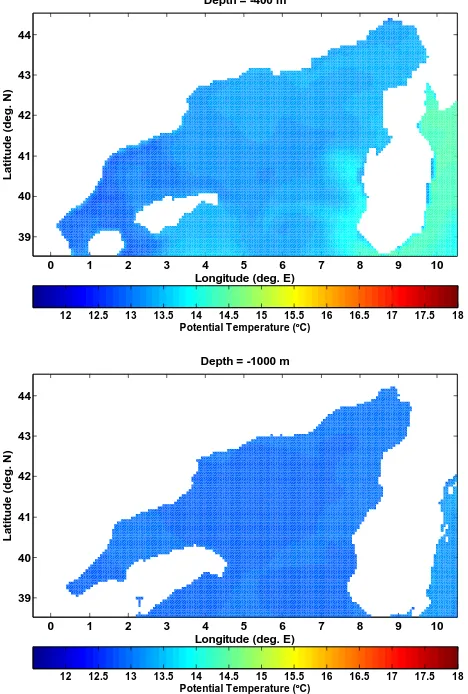
Fig. 10 Initial Conditions for potential temperature: at 400-m depth (upper panel) and at 1000-m depth (lower panel), from December of the 8th_{year of the Mediterranean Sea OGCM}

climatological integration(source data: Mediterranean Forecasting System, 2002).

23

Fig. 10. Initial Conditions for potential temperature: at 400-m depth (upper panel) and at 1000-m depth (lower panel), from December of the 8th year of the Mediterranean Sea OGCM climatological in-tegration (source data: Mediterranean Forecasting System, 2002).

the other hand, the winds over the eastern region of Sardinia and Corsica blow eastward during both months. In general, the climatological winds are more intense during February than during August.

3.1.3 Evaporation rate minus precipitation

The spatial distribution of evaporation rate minus precipi-tation (E-P) for February and August is shown in Fig. 4. This figure illustrates the freshwater losses affecting the en-tire NMS model’s domain, especially intense in the Gulf of Lions and between Minorca and Sardinia. During February there is a clear southwest-northeast gradient, while during August this gradient is not so well defined.

3.1.4 Sea surface temperature and salinity

The sea surface temperature and salinity from the MED6 monthly climatology for February and August are shown in

0 1 2 3 4 5 6 7 8 9 10

39 40 41 42 43 44

Latitu

d

e

(d

e

g

.

N

)

Depth = -30 m

1m/s

Salinity (psu)

36 36.5 37 37.5 38 38.5 39

0 1 2 3 4 5 6 7 8 9 10

39 40 41 42 43 44

Latitu

d

e

(d

e

g

.

N

)

Depth = -160 m

1m/s

Salinity (psu)

36 36.5 37 37.5 38 38.5 39

Fig. 11 Velocity field and horizontal distribution of salinity: at 30-m depth (upper panel) and at 160-m depth (lower panel) during August from the climatological experiment.

24

Fig. 11. Velocity field and horizontal distribution of salinity: at 30-m depth (upper panel) and at 160-m depth (lower panel) during August from the climatological experiment.

Figs. 5 and 6. The sea surface thermal structure over the NMS model’s domain in February is moderately homoge-neous, particularly in the northern area that extends from the Balearic Islands to the Ligurian Sea. In this region, the tem-perature does not exceed 13.5◦C. The coldest waters (13◦C) are found on the Ligurian Sea, Gulf of Lions and the north part of the Catalan Sea. In contrast, the warmer waters (14◦– 14.5◦C) are found over the whole southern part of the do-main. During August, this thermal structure clearly changes reaching temperatures between 20◦_{C (particularly over the}

Gulf of Lions) and 25o_{C (on the south side of the NMS}

(8)

0 1 2 3 4 5 6 7 8 9 10 39

40 41 42 43 44

Latitu

d

e

(d

e

g

.

N

)

Depth = -400 m

1m/s

Salinity (psu)

36 36.5 37 37.5 38 38.5 39

0 1 2 3 4 5 6 7 8 9 10

39 40 41 42 43 44

Latitu

d

e

(d

e

g

.

N

)

Depth = -1000 m

1m/s

Salinity (psu)

36 36.5 37 37.5 38 38.5 39

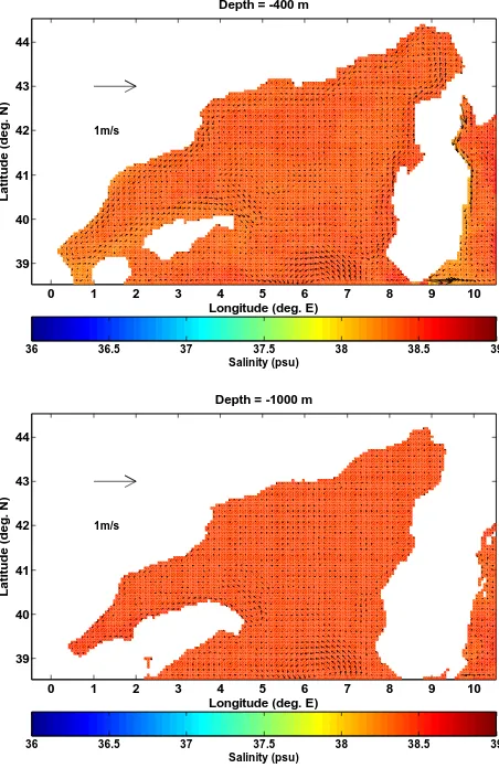
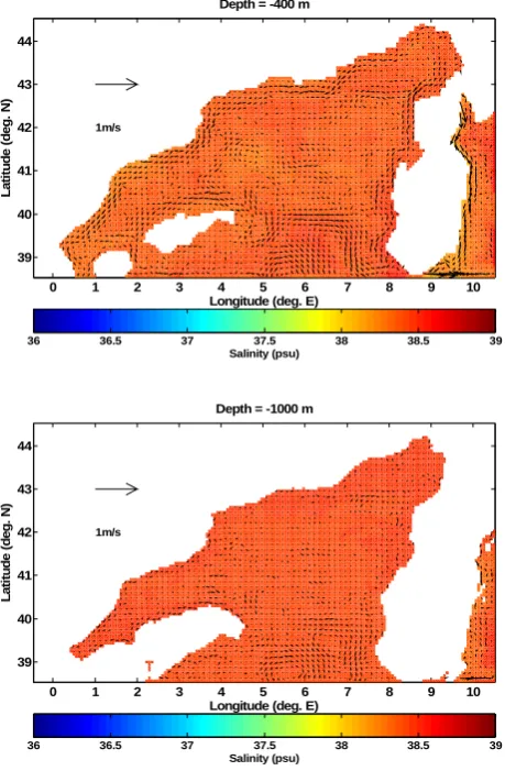
Fig. 12 Velocity field and horizontal distribution of salinity: at 400-m depth (upper panel) and at 1000-m depth (lower panel) during August from the climatological experiment.

25

Fig. 12. Velocity field and horizontal distribution of salinity: at 400-m depth (upper panel) and at 1000-400-m depth (lower panel) during August from the climatological experiment.

salinity values between 37.2 and 37.8 over the southern re-gion (between∼38.5◦ and 41◦N), and 3) salinity values of 38 on the region north of 41◦N. In the latter, the exceptions are the Gulf of Lions shelf and the west part of the Ligurian Sea where salinities of 37.8 are observed. From a seasonal point of view, the sea surface salinity on the NMS model’s domain does not show significant variations from one month to another. However, it is evident that waters with salinities between 37.6 and 37.8 invade the northern region mainly in August.

3.1.5 River runoffs

According to the Compagnie Nationale du Rhône (Younes et al., 2003), the Rhone River runoffs, from 1996 to 2000, var-ied from a monthly average maximum of 2522 m3s−1 (De-cember) to a minimum 943 m3s−1(August) with an annual mean value of 1745 m3s−1. During the same period, the Ebro River annual mean runoffs; obtained from the Confederación Hidrográfica del Ebro (Jordà, 2005), was 315 m3s−1, with

0 1 2 3 4 5 6 7 8 9 10

39 40 41 42 43 44

Latitu

d

e

(d

e

g

.

N

)

Depth = -30 m

1m/s

Salinity (psu)

36 36.5 37 37.5 38 38.5 39

0 1 2 3 4 5 6 7 8 9 10

39 40 41 42 43 44

Latitu

d

e

(d

e

g

.

N

)

Depth = -160 m

1m/s

Salinity (psu)

36 36.5 37 37.5 38 38.5 39

Fig. 13 Velocity field and horizontal distribution of salinity: at 30-m depth (upper panel) and at 160-m depth (lower panel) during November from the climatological experiment.

26

Fig. 13. Velocity field and horizontal distribution of salinity: at 30-m depth (upper panel) and at 160-m depth (lower panel) during November from the climatological experiment.

a monthly average maximum of 689 m3s−1(January) and a minimum of 128 m3s−1(August).

3.2 Initial conditions

(9)

0 1 2 3 4 5 6 7 8 9 10 39

40 41 42 43 44

Latitu

d

e

(d

e

g

.

N

)

Depth = -400 m

1m/s

Salinity (psu)

36 36.5 37 37.5 38 38.5 39

0 1 2 3 4 5 6 7 8 9 10

39 40 41 42 43 44

Latitu

d

e

(d

e

g

.

N

)

Depth = -1000 m

1m/s

Salinity (psu)

36 36.5 37 37.5 38 38.5 39

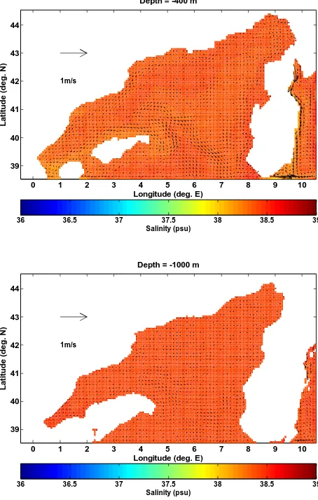
Fig. 14 Velocity field and horizontal distribution of salinity: at 400-m depth (upper panel) and at 1000-m depth (lower panel) during November from the climatological experiment.

27

Fig. 14. Velocity field and horizontal distribution of salinity: at 400-m depth (upper panel) and at 1000-400-m depth (lower panel) during November from the climatological experiment.

approximately latitudinal with higher salinity values at the northern areas, especially inside the large cyclonic gyre. In contrast, the western part of the Tyrrhenian Sea does not show this latitudinal gradient but its salinity values are com-parable to those inside the cyclonic gyre. On the other hand, the horizontal distribution of potential temperature (Figs. 9 and 10) shows the lower values (between ∼13-14◦C) over the northern part of the Catalan Sea, the Gulf of Lions, the Ligurian Sea and particularly, inside the large cyclonic gyre. In contrast, the higher temperatures (between∼14.5-17◦_C)

are observed on the southern part of the NMS model domain, including the southwestern area of the Tyrrhenian Sea.

4 Model results and discussions

In the following paragraphs the NMS model results for a typ-ical summer (August), autumn (November), winter (Febru-ary) and spring (May) month will be analyzed. These

re-0 1 2 3 4 5 6 7 8 9 10

39 40 41 42 43 44

L

a

ti

tu

d

e

(d

e

g

.

N

)

Depth = -30 m

1m/s

Salinity (psu)

36 36.5 37 37.5 38 38.5 39

0 1 2 3 4 5 6 7 8 9 10

39 40 41 42 43 44

L

a

ti

tu

d

e

(d

e

g

.

N

)

Depth = -160 m

1m/s

Salinity (psu)

36 36.5 37 37.5 38 38.5 39

Fig. 15 Velocity field and horizontal distribution of salinity: at 30-m depth (upper panel) and at 160-m depth (lower panel) during February from the climatological experiment.

28

Fig. 15. Velocity field and horizontal distribution of salinity: at 30-m depth (upper panel) and at 160-m depth (lower panel) during February from the climatological experiment.

sults correspond to the climatological integration of the NMS model, which was run for 12 years with forcing and initial conditions described in Sect. 3 and model parameters sum-marized in Table 1.

According to this climatological experiment, during Au-gust the northern part of the NMS model’s domain is charac-terized by a well-defined large-scale cyclonic circulation at least up to 400-m depth (Fig. 11 and Fig. 12, upper panel). In this month, there is clear evidence of the Gulf of Lions cyclonic gyre centered at 42◦_N–5◦_{E and the Northern}

(10)

0 1 2 3 4 5 6 7 8 9 10 39

40 41 42 43 44

L

a

ti

tu

d

e

(d

e

g

.

N

)

Depth = -400 m

1m/s

Salinity (psu)

36 36.5 37 37.5 38 38.5 39

0 1 2 3 4 5 6 7 8 9 10

39 40 41 42 43 44

L

a

ti

tu

d

e

(d

e

g

.

N

)

Depth = -1000 m

1m/s

Salinity (psu)

36 36.5 37 37.5 38 38.5 39

Fig. 16 Velocity field and horizontal distribution of salinity: at 400-m depth (upper panel) and at 1000-m depth (lower panel) during February from the climatological experiment.

29

Fig. 16. Velocity field and horizontal distribution of salinity: at 400-m depth (upper panel) and at 1000-400-m depth (lower panel) during February from the climatological experiment.

south and to the north of the Balearic Islands), appears as a continuous northeastwards flow closing the cyclonic circu-lation that is delimited southward by an oceanic front. In contrast, the southern region of the NMS model’s domain is dominated principally by mesoscale eddies with different sign and dimension. These eddies, as it can be seen from the distribution of salinity, appear to play an important role in the advection of water of Atlantic origin towards the north. Con-cerning the circulation over the part of the Tyrrhenian Sea considered in this study, there is indication that, in the upper layers (see Fig. 11, upper panel) the flow is mainly north-wards while it is southnorth-wards in the lower layers (see Fig. 11, lower panel and Fig. 12) along the Corsican and Sardinian coasts. In general, it is evident that Levantine Intermediate Water (LIW) (Fig. 12, upper panel) and Western Mediter-ranean Deep Water (WMDW) (Fig. 12, lower panel), possi-bly constrained by the bottom topography, follow essentially a cyclonic path.

During November the large-scale cyclonic circulation is

0 1 2 3 4 5 6 7 8 9 10

39 40 41 42 43 44

L

a

ti

tu

d

e

(d

e

g

.

N

)

Depth = -400 m

1m/s

Salinity (psu)

36 36.5 37 37.5 38 38.5 39

0 1 2 3 4 5 6 7 8 9 10

39 40 41 42 43 44

L

a

ti

tu

d

e

(d

e

g

.

N

)

Depth = -1000 m

1m/s

Salinity (psu)

36 36.5 37 37.5 38 38.5 39

Fig. 18 Velocity field and horizontal distribution of salinity: at 400-m depth (upper panel) and at 1000-m depth (lower panel) during May from the climatological experiment.

31

Fig. 17. Velocity field and horizontal distribution of salinity: at 30-m depth (upper panel) and at 160-30-m depth (lower panel) during May from the climatological experiment.

basically the same as in August but, in this case, a stretching around 42◦_N–4◦₄₅0_{E is displayed (Fig. 13). This stretching,}

observed as a large meander invading the northern part, ap-pears to be associated with the Gulf of Lions cyclonic gyre, which is relatively well-defined. Other significant features in this month are the presence of several mesoscale eddies along the western side of the Corsica and the occurrence of a cyclonic gyre on the western Tyrrhenian Sea, specifically to the north of the Strait of Bonifacio. Over the southern region of the NMS model’s domain, mesoscale eddies are as in Au-gust the most important dynamic characteristic. In general, also during November, the LIW (Fig. 14, upper panel) and WMDW (Fig. 14, lower panel) follow a cyclonic path.

(11)

0 1 2 3 4 5 6 7 8 9 10 39

40 41 42 43 44

L

a

ti

tu

d

e

(d

e

g

.

N

)

Depth = -400 m

1m/s

Salinity (psu)

36 36.5 37 37.5 38 38.5 39

0 1 2 3 4 5 6 7 8 9 10

39 40 41 42 43 44

L

a

ti

tu

d

e

(d

e

g

.

N

)

Depth = -1000 m

1m/s

Salinity (psu)

36 36.5 37 37.5 38 38.5 39

Fig. 18 Velocity field and horizontal distribution of salinity: at 400-m depth (upper panel) and at 1000-m depth (lower panel) during May from the climatological experiment.

31

Fig. 18. Velocity field and horizontal distribution of salinity: at 400-m depth (upper panel) and at 1000-400-m depth (lower panel) during May from the climatological experiment.

and three large gyres are displayed on the Ligurian Sea and offshore the Gulf of Lions where a large anticyclonic gyre closes to the Gulf of Lions cyclonic gyre is present. Further-more, mesoscale eddies detected up to 160-m depth prevail over the entire southern region, with evident effect, at least in the upper layer, on the southern part of the large-scale cy-clonic circulation. Also, in this season, the cycy-clonic gyre on the western side of the Tyrrhenian Sea is present. Below this depth, the LIW (Fig. 16, upper panel) and WMDW (Fig. 16, lower panel) follow, as in August and November, essentially a cyclonic path.

Finally, during May, at 30-m depth (Fig. 17, upper panel), the NC becomes relatively more intense than in February but even less strong than during August and November. In this month, although the large gyres in the Ligurian Sea and in the Gulf of Lions open sea are less evident, the large scale cyclonic circulation is not completely reestablished. In ad-dition, over the southern part of the Catalan Sea, meanders and mesoscale eddies have been developed. Furthermore, on

the southern region of the NMS model’s domain, the number of mesoscale eddies have diminished and the cyclonic gyre on the western side of the Tyrrhenian Sea has disappeared. At 160-m depth (Fig. 17, lower panel), the large-scale cy-clonic circulation is basically as in the previous months but, mesoscale eddies have almost disappeared from the southern region of the NMS model’s domain. Below this depth, the circulation of both LIW (Fig. 18, upper panel) and WMDW (Fig. 18, lower panel) is also cyclonic.

From these results, it is evident that the circulation in the Northwestern Mediterranean Sea is more complicated than that published by early works (among other, Nielsen, 1912; Allain, 1960, Furnestin, 1960; W¨ust, 1961; Ovchinnikov, 1966). In this context, recent studies (WMCE Group, 1994; EUROMODEL Group, 1995) have pointed out that because of scarcity and spacing of ocean stations, early studies of the area have presented a simple pattern of the circulation, which is more complex and driven by a combination of fac-tors and time scales. Several observational studies carried out in the nineties (Send et al., 1999) and during the last years have showed evidence of important mesoscale activity (fronts, meanders, eddies, filaments, etc.) affecting the cir-culation at local, sub-basin and basin scale. More recently, in order to investigate if the intrinsic ocean variability could be a source of interannual variability, Fern´andez et al. (2005) implemented an eddy permitting rigid lid ocean model (the DieCAST model) in the whole Mediterranean Sea. The model results showed the seasonality of some currents, an important eddy field and numerous fronts distributed all over the Mediterranean Sea. In the present study, an eddy per-mitting free surface ocean model (the POM model) forced at the surface with climatological heat fluxes and wind stress, and on the open lateral boundaries with temperature, salinity and velocity fields obtained from a Mediterranean Sea gen-eral circulation model, has confirmed that: 1) the large-scale cyclonic circulation in the Northwestern Mediterranean Sea changes from one season to another; 2) the mesoscale struc-ture is, during all year, a significant characteristic in this re-gion of the Mediterranean Sea, and 3) the circulation of Lev-antine Intermediate Water (LIW) and Western Mediterranean Deep Water (WMDW) is basically cyclonic during all year.

5 Conclusions

(12)

Acknowledgements. We acknowledge the Mediterranean Forecast-ing System (MFS) for providForecast-ing data for this study and several of the participants in projects MFSPP and MFSTEP for providing advice. M. Ahumada was supported by the Universidad del Mar and the Secretar´ıa de Educación Pública (SEP) of Mexico through the PROMEP program. This work was performed in a Silicon Graphic Origin 300 from the Computation Center of the Universitat Politècnica de Catalunya.

Edited by: N. Pinardi

References

Alvarez, A., Tintoré, J., Holloway, G., Eby, M., and Beckers, J. M.: Effect of topographic stress on circulation in the western Mediterranean, J. Geophys. Res., 99, 16 053–16 064, 1994. Allain, C.: Topographie dynamique et courants généraux dans le

bassin occidental de la M´editerran´ee, Rev. Trav. Inst. Peches Marit., 24(1), 121–145, 1960.

Astraldi, M. and Gasparini, G. P.: The Seasonal Characteristics of the Circulation in the North Mediterranean Basin and Their Rela-tionship with the Atmospheric-Climate Conditions, J. Geophys. Res., 97, 9531–9540, 1992.

Beckers J. M.: Application of the GHER 3D general circulation model to the western Mediterranean, J. Mar. Syst., 1, 315–322, 1991.

Beckers, J. M., Rixen, M., Brasseur, P., Brankart, J. M., Elmous-saoui, A., Cr´epon, M., Herbaut, Ch., Martel, F., Van den Berghe, F., Mortier, L., Lascaratos, A., Drakopoulos, P., Korres, G., Nit-tis, K., Pinardi, N., Masetti, E., Castellari, S., Carini, P., Tintor´e, J., Alvarez, A., Monserrat, S., Parrilla, D., Vautard, R., and Spe-ich, S.: Model intercomparison in the Mediterranean: MEDMEX simulations of the seasonal cycle, J. Mar. Syst., 33–34, 215–251, 2002.

Bergamasco, A., Malanotte-Rizzoli, P., Thacker, W. C., and Long, R.B.: The seasonal steady circulation of the Eastern Mediter-ranean determined with the adjoint method, Deep-Sea Res., 40(6), 1269–1298, 1993.

Blumberg, A. and Mellor, G.: A Description of a Three-Dimensional Coastal Ocean Circulation Model, in: Three-Dimensional Coastal Ocean Models, Coastal Estuarine Science, edited by: Heaps, N. S., American Geophysical Union, 1–16, 1987.

Brankart, J. M. and Brasseur, P.: The general circulation in the Mediterranean Sea: a climatological approach, J. Mar. Syst., 18, 41–70, 1998.

Brenner, S.: High-resolution nested model simulations of the clima-tological circulation in the southeastern Mediterranean Sea, Ann. Geophys., 20, 267–280, 2002.

Castellari, S., Pinardi, N., and Leaman, K.: A model study of air-sea interactions in the Mediterranean Sea, J. Mar. Syst., 18, 89–114, 1998.

Demirov, E. and Pinardi, N.: Simulation of the Mediterranean Sea circulation from 1979 to 1993: Part I. The interannual variability, J. Mar. Syst., 33, 23–50, 2002.

Drakopoulos, P. G. and Lascaratos, A.: Modelling the Mediter-ranean Sea: climatological forcing, J. Mar. Syst., 20, 157–173, 1999.

Echevin V., Cr`epon, M., and Mortier, L.: Simulation and analysis of the mesoscale circulation in the northwestern Mediterranean Sea, Ann. Geophys., 21, 281–297, 2002.

EUROMODEL Group: Progress from 1989 to 1992 in understand-ing the general circulation of the Western Mediterranean Sea, Oceanologica Acta, 18, 255–271, 1995.

Fern´andez, V., Dietrich, D. E., Haney, R. L., and Tintor´e, J.: Mesoscale, seasonal and interannual variability in the Mediter-ranean Sea using a numerical ocean model, Progress in Oceanog-raphy, 1–20, 2005.

Furnestin, J.: Hydrologie de la M´editerran´ee occidentale (Golfe du Lion, Mer Catalane, Mer d’Alboran, Corse orientale), 14 Juin–20 Juillet 1957, Rev. Trav. Inst. Peches Marit., 24(1), 5–104. 1960. Gasparini, G. P., Zodiatis, G., Astraldi, M., Galli C., and

Sparnoc-chia, S.: Winter intermediate water lenses in the Ligurian Sea, J. Mar. Syst., 20, 319–332, 1999.

Haines, K. and Wu, P.: A modelling study of the thermohaline cir-culation of the Mediterranean Sea: water formation and disper-sal, Oceanologica Acta, 18(4), 401–417, 1995

Heburn, G. W.: The dynamics of the western Mediterranean Sea: A wind forced case study, Ann. Geophys., 5B, 61–74, 1987. Herbaut, C., Mortier, L., and Cr´epon, M.: A sensitivity study of

the General Circulation of the Western Mediterranean Sea. Part I: The Response to Density Forcing through the Straits, J. Phys. Oceanogr., 26, 65–84, 1996.

Herbaut, C., Martel, F., and Cr´epon, M.: A sensitivity study of the General Circulation of the Western Mediterranean Sea. Part II: The Response to Atmospheric Forcing, J. Phys. Oceanogr., 26, 65–84, 1997.

Jord`a, S. G.: Towards Data Assimilation in the Catalan Continental Shelf: From data analysis to optimization methods. Ph.D. Thesis. Universitat Polit`ecnica de Catalunya, 333 p., 2005.

Korres, G. and Lascaratos, A.: A one-way nested eddy resolving model of the Aegean and Levantine basins: implementation and climatological runs, Ann. Geophys., 21, 205–220, 2003. Lascaratos, A. and Nittis, K.: A high-resolution three-dimensional

numerical study of intermediate water formation in the Levantine Sea, J. Geophys. Res., 103, 18 497–18 511, 1998.

La Violette, P. E.: The Western Mediterranean Circulation Experi-ment (WMCE): Introduction, J. Geophys. Res., 95(C2), 1511– 1514, 1990.

Malanotte-Rizzoli, P. and Bergamasco, A.: The general circulation of the eastern Mediterranean. Part I: The barotropic wind driven circulation, Oceanologica Acta, 12, 335–351, 1989.

Malanotte-Rizzoli, P. and Bergamasco, A.: The wind and thermally driven circulation of the eastern Mediterranean Sea. Part II: The baroclinic case, Dyn. Atmos. Oceans, 15, 355–419, 1991. Madec, G., Chartier, M., and Cr´epon, M.: The effect of the

thermo-haline forcing variability on deep-water formation in the western Mediterranean Sea: a high-resolution three-dimensional numeri-cal study, Dyn. Atmos. Oceans, 15(3–5), 301–332, 1991a. Madec, G., Delecluse, P., and M. Cr´epon, M.: Numerical study of

deep-water formation in the western Mediterranean Sea, J. Phys. Oceanogr., 26, 1349–1371, 1991b.

Menzin, A. B. and Moskalenko, L. V.: Calculation of wind driven currents in the Mediterranean Sea by the electrical simulation method, Oceanologica, 22, 537–540, 1982.

(13)

Mellor, G.: User’s Guide for a Three-Dimensional Primitive Equa-tion, Numerical Ocean Model. Princeton University, Princeton, N.J., 1–56, 2004

Mellor, G. and Blumberg, A. F.: Modeling Vertical and Horizontal Diffusivities with the Sigma Coordinate System, Mon. Weather Rev., 113, 1279–1383, 1986.

Mellor, G. and Yamada, T.: Development of a turbulence closure sub-model for geophysical fluid problems, Rev. Geophys., 20, 851–875, 1982

Millot, C.: Circulation in the Western Mediterranean Sea, Oceanologica Acta, 10, 143–149, 1987.

Millot, C.: Mesoscale and seasonal variability of the circulation in the western Mediterranean, Dyn. Atmos. Oceans, 15, 179–214, 1991.

Millot, C.: Circulation in the Western Mediterranean Sea, J. Mar. Syst., 20, 423–442, 1999.

Molcard, A., Pinardi, N., Iskandarani, M., and Haidvogel, D. B.: Wind driven general circulation of the Mediterranean Sea simulated with a Spectral Element Ocean Model, Dyn. Atmos. Oceans, 35, 97–130, 2002.

Nielsen, J. N.: Hydrography of the Mediterranean and Adjacent Waters, Report on the Danish Oceanography Expeditions, 77– 192, 1912.

Ovchinnikov, I. M.: Circulation in the surface and intermediate lay-ers of the Mediterranean Sea, Oceanology, 6, 48–59, 1966. Pinardi, N. and Navarra, A.: Baroclinic wind adjustment processes

in the Mediterranean Sea, Deep-Sea Res., 40, 1299–1326, 1993. Pinardi, N. and Masetti, E.: Variability of the large-scale general circulation of the Mediterranean Sea from observations and mod-elling: a review, Palaeogeography, Palaeoclimatology, Palaeoe-cology, 158, 153–173, 2000.

Pinardi, N., Allen, I., Demirov, E., De Mey, P., Korres, G., Las-caratos, A., Le Traon, P.Y., Maillard, C., Manzella, G., and Tziavos, C.: The Mediterranean ocean forecasting system: first phase of implementation (1998–2001), Ann. Geophys., 21, 3–20, 2003.

Roussenov, V., Stanev, E., Artale, V., and Pinardi, N.: A seasonal model of the Mediterranean Sea general circulation, J. Geophys. Res., 100, 13 515–13 538, 1995.

Send, U., Font, J., Krahmann, G., Millot, C., Rhein, M., and Tin-tor´e, J.: Recent advances in observing the physical oceanography of the western Mediterranean Sea, Progress Oceanogr., 44, 37– 64, 1999.

Smagorinsky, J.: General Circulation Experiments with the Primi-tive Equations, Mon. Weather Rev., 91(3), 99–165, 1963. Sorgente, R., Drago, A. F., and Ribotti, A.: Seasonal variability in

the Central Mediterranean Sea circulation, Ann. Geophys., 21, 299–322, 2003.

Stanev, E. V., Friedrich, H. J., and Botev, S.: On the seasonal re-sponse of intermediate and deep water to surface forcing in the Mediterranean Sea, Oceanologica Acta, 12, 141–149, 1989. Tonani, M.: Studi della predicibilit`a della circolazione del Mar

Mediterraneo. Ph.D. Thesis. Universit`a degli Studis di Bologna, 139 p., 2003.

Tziperman, E. and Malanotte-Rizzoli, P.: The climatological sea-sonal circulation of the Mediterranean Sea, J. Mar. Res., 49, 411– 434, 1991.

WMCE Group: Seasonal and Interannual Variability of the Western Mediterranean Sea, Coastal and Estuarine Studies, edited by: La Violette, P. E., American Geophysical Union, 6, 373, 1994. Wu, P. and Haines, K.: Modelling the dispersal of Levantine

Inter-mediate Water and its role in Mediterranean deep-water forma-tion, J. Geophys. Res., 101(C3), 6591–6607, 1996.

W¨ust, G.: On the vertical circulation of the Mediterranean Sea, J. Geophys. Res., 66, 3261–3271, 1961.

Younes, W. A. N., Bensoussan, N., Romano, J. C., Arlhac, D., and Lafont, M. G.: Seasonal and Interannual variations (1996–2000) of the coastal waters east of the Rhone River mouth as indicated by the SORCOM series, Oceanologica Acta, 26, 311–321, 2003. Zavatarelli, M. and Mellor, G.: A numerical study of the Mediter-ranean Sea Circulation, J. Phys. Oceanogr., 25, 1384–1414, 1995.

Zavatarelli, M., Baretta, J. W., Baretta-Bekker, J. G., and Pinardi, N.: The dynamics of the Adriatic Sea ecosystem: An idealized model study, Deep-Sea Res., 47, 937–970, 2000.

Zavatarelli, M., Pinardi, N., Kourafalou, V. H., and Maggiore, A.: Diagnostic and prognostic model studies of the Adriatic Sea gen-eral circulation: Seasonal variability, J. Geophys. Res., 107, 1– 20, 2002.

References

Alvarez, A., Tintor´e, J., Holloway, G., Eby, M., and Beckers, J. M.: Effect of topographic stress on circulation in the western Mediterranean, J. Geophys. Res., 99, 16 053–16 064, 1994. Allain, C.: Topographie dynamique et courants g´en´eraux dans le