www.clim-past.net/11/605/2015/ doi:10.5194/cp-11-605-2015
© Author(s) 2015. CC Attribution 3.0 License.
Interannual climate variability seen in the Pliocene Model
Intercomparison Project
C. M. Brierley
Department of Geography, University College London, Gower St, London, WC1E 6BT, UK Correspondence to: C. M. Brierley ([email protected])
Received: 8 August 2014 – Published in Clim. Past Discuss.: 17 September 2014 Revised: 10 February 2015 – Accepted: 23 February 2015 – Published: 27 March 2015
Abstract. Following reconstructions suggesting weakened temperature gradients along the Equator in the early Pliocene, there has been much speculation about Pliocene climate variability. A major advance for our knowledge about the later Pliocene has been the coordination of mod-elling efforts through the Pliocene Model Intercomparison Project (PlioMIP). Here the changes in interannual modes of sea surface temperature variability will be presented across PlioMIP. Previously, model ensembles have shown little con-sensus in the response of the El Niño–Southern Oscillation (ENSO) to imposed forcings – either for the past or future. The PlioMIP ensemble, however, shows surprising agree-ment, with eight models simulating reduced variability and only one model indicating no change. The Pliocene’s ro-bustly weaker ENSO also saw a shift to lower frequencies. Model ensembles focussed on a wide variety of forcing sce-narios have not yet shown this level of coherency. Nonethe-less, the PlioMIP ensemble does not show a robust response of either ENSO flavour or sea surface temperature variabil-ity in the tropical Indian and North Pacific oceans. Existing suggestions linking ENSO properties to to changes in zonal temperature gradient, seasonal cycle and the elevation of the Andes Mountains are investigated, yet prove insufficient to explain the consistent response. The reason for this surpris-ingly coherent signal warrants further investigation.
1 Introduction
The Pliocene is an interesting time period for palaeoclimate research. It was the last time that atmospheric carbon dioxide concentrations were similar to their present, elevated values (Masson-Delmotte et al., 2013; Fedorov et al., 2013). Sea
Zhang et al. (2012b) investigate the ENSO and mean equa-torial SST gradient in one simulation performed as part of the Pliocene Model Intercomparison Project (PlioMIP) with standard model physics. They found that the NorESM-L model (Table 1) simulates a reduction in zonal SST gradi-ent as well as a weakening of ENSO amplitude when forced by mid-Piacenzian boundary conditions. Here I describe the climate variability of all the model simulations that were per-formed as part of the same PlioMIP ensemble. This work is motivated in part by a desire to explore whether this result holds across the ensemble and in part by academic curiosity about past climate variability.
The remainder of this article will first give a brief overview of the PlioMIP ensemble (Sect. 2.1) and detail the data analy-sis methods used (Sect. 2.2). The results section will describe Pliocene climate variability in the tropical Pacific (Sect. 3.1), Indian (Sect. 3.2) and North Pacific (Sect. 3.3) oceans. I will then discuss the significance, statistical (Sect. 4.3) and other-wise, of these results and attempt to provide an explanation for them.
2 Methods 2.1 PlioMIP
The PlioMIP ensemble has been created to investigate the climate of the warm mid-Piacenzian. Here, I utilise only the contributions to experiment 2, which requires the use of cou-pled climate models (Haywood et al., 2013). Nine climate models from different institutions around the world have con-tributed simulations to the project (Table 1). Each model has performed a preindustrial simulation following the CMIP5 (Coupled Model Intercomparison Project phase 5) protocol. They also perform a simulation representing the average in-terglacial conditions between 3.264 and 3.025 million years ago (Haywood et al., 2011). This involves increasing the car-bon dioxide concentrations (278–405 ppm) and altering the prescribed boundary conditions in line with the Pliocene Re-search Interpretation and Synoptic Mapping reconstructions (PRISM; Dowsett et al., 2012). A full description of the PlioMIP experiment protocols are given by Haywood et al. (2011), and the implementation of them for each model is given by the accompanying reference in Table 1.
The simulations in the PlioMIP ensemble have been pre-viously investigated. In addition to single-model descriptions (listed in Table 1), there have been coordinated studies across the whole ensemble. The large-scale features of the ensem-ble are described in Haywood et al. (2013). The simulations warm between 1.8 and 3.6◦C on the global mean. Two of the individual model papers describe aspects of the climate vari-ability (Rosenbloom et al., 2013; Zheng et al., 2013). Addi-tionally, Zhang et al. (2012b) focus specifically on the ENSO simulation of NorESM-L. They find substantially weaker variability in the Niño 3.4 region, which they associate with
the reduced equatorial SST gradient in the Pliocene simula-tion. An analysis of the climate variability across the PlioMIP ensemble using a unified methodology has not been previ-ously performed.
2.2 Data analysis
Many differing approaches have been devised to study cli-mate variability. Two distinct techniques to detect modes of variability are followed here: principal component analysis and index-driven metrics. Both techniques involve comput-ing the average annual cycle and lookcomput-ing at anomalies from that. The lengths of records archived in the PlioMIP database is at best 200 years of sea surface temperatures; at worst, 100 years are available (see Table 1). As these time series represent “equilibrium” states from the end of long simu-lations, they should have quasi-stable climates. The annual cycle was computed as the average of the whole available record for each model grid point and month of the year. Sea surface temperature anomalies (SSTAs) from this annual cy-cle were computed.
The area-weighted average SSTAs were computed over several standard regions. The Niño 3.4 region is used for the majority of the analysis, which is defined as 170–120◦W, 5◦S–5◦N. Niño 3 (150–90◦W, 5◦S–5◦N) and Niño 4 (160◦E–150◦W, 5◦S–5◦N) were also computed. They show a similar response to the Niño 3.4 indices, so the following will concentrate on just the Niño 3.4 region. However, Ren and Jin (2011) devised a simple transformation of the Niño 3,
N3, and Niño 4,N4, regions to track two different types of ENSO. These are discussed further in Sect. 3.1.4. This trans-formation creates two new indices,NCTandNWP, character-ising the cold-tongue and warm-pool types of El Niño, re-spectively (Eq. (1); Ren and Jin, 2011).
(
NCT=N3−αN4
NWP=N4−αN3
α=
(2
5, N3N4>0
0, otherwise (1)
Trenberth (1997) advocated using a 5-month running win-dow to smooth ENSO SSTA indices. Some ensemble mem-bers exhibit high sub-seasonal variability (e.g. NorESM-L; Zhang et al., 2012b). Also the normalisation (described be-low) of the power spectra would be distorted by variations in the annual cycle. Therefore, smoothing is instead performed with a Lanczos low-pass filter of 18 months (UCAR, 2014).
The dipole mode index is used to look at Indian Ocean variability (Saji et al., 1999; Cai et al., 2013). It is defined as the difference between area-weighted average temperature anomalies between the west (50–70◦E, 10◦S–10◦N) and the south-east (90–110◦W, 10–0◦S) Indian Ocean.
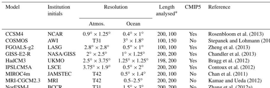
Table 1. Simulations contributing to the PlioMIP ensemble (see Sect. 2.1 and Haywood et al., 2013, for details). The resolution given relates to the deep tropics for models with a varying ocean resolution. The length analysed represents the number of model years uploaded to the PlioMIP database – the simulation is often much longer.
Model Institution Resolution Length CMIP5 Reference
initials analysed∗
Atmos. Ocean
CCSM4 NCAR 0.9◦×1.25◦ 0.4◦×1◦ 200, 100 Yes Rosenbloom et al. (2013) COSMOS AWI T31 3◦×1.8◦ 100, 150 No Stepanek and Lohmann (2012) FGOALS-g2 LASG 2.8◦×2.8◦ 0.5◦×1◦ 100, 100 Yes Zheng et al. (2013)
GISS-E2-R NASA/GISS 2◦×2.5◦ 1◦×1.25◦ 200, 200 Yes Chandler et al. (2013) HadCM3 UKMO 2.5◦×3.75◦ 1.25◦×1.25◦ 198, 200 Yes Bragg et al. (2012) IPSLCM5A LSCE 3.75◦×1.9◦ 0.5◦×2◦ 200, 200 Yes Contoux et al. (2012) MIROC4m JAMSTEC T42 0.5◦×1.4◦ 200, 100 No Chan et al. (2011) MRI-CGCM2.3 MRI T42 0.5–2.5◦ 200, 200 No Kamae and Ueda (2012) NorESM-L BCCR T31 1.5◦×3◦ 200, 200 No Zhang et al. (2012a) ∗Preindustrial followed by Pliocene simulation.
The first two EOFs of the tropical Pacific (140◦E–80◦W, 15◦S–15◦N) and North Pacific (110◦E–90◦W, 20–65◦N) are also computed along with the global patterns. Power et al. (2013) found a robust future change in the ENSO structure by creating ensemble-averaged EOF patterns. To facilitate this, the EOFs are computed on their native grid and then bilin-early interpolated onto the 2◦×2◦ grid of the ERSST ob-servations (Smith et al., 2008). The EOF patterns are then normalised by the spatial standard deviation of the region (Power et al., 2013).
Spectral analysis is used to investigate the frequency properties of the interannual variability. The power spec-tra are computed from a smoothed and tapered periodogram (UCAR, 2014). To isolate the temporal properties from any amplitude changes, all time series are normalised by their own standard deviations. This applies to both the SST indices and the principal components, both of which are low-pass fil-tered at 18 months (as described above) to avoid signatures associated with annual cycle changes. The dominant period (as shown in Tables 2 and 3) is defined as the period with the maximal power density in the spectrum. Ensemble average spectra are computed after this normalisation.
3 Results
3.1 Tropical Pacific
The best-studied mode of interannual climate variability is the El Niño–Southern Oscillation (ENSO). However, this does not mean it is yet well understood. Future projections of ENSO are model-dependent – with some models showing increasing variability and others showing reductions (Collins et al., 2010). There are a plethora of metrics and approaches to investigate how well models simulate the present-day properties of ENSO. Novel approaches have started to focus
on the underlying physical processes, rather than the emer-gent climate variability that will be the focus of this work (e.g. Jin et al., 2006). The model representation of ENSO has improved in the CMIP5 compared to CMIP3 (Bellenger et al., 2013), with more models showing a realistic power spectrum (Flato et al., 2013). Power et al. (2013) were able to show the benefit of separating the various of aspects ENSO during model intercomparison by finding a robust pattern of change in 21st-century simulations. Motivated by this result, combined with the fact that the PlioMIP models show a large diversity of ENSO simulation quality, each property is inves-tigated independently of the others. The method described above isolates the amplitude, frequency and structure. This means that, say, the reduction in amplitude noted by Zhang et al. (2012b) will not interfere with the spatial pattern asso-ciated with an El Niño. Using a composite El Niño approach with a predefined threshold instead (e.g. Haywood et al., 2007) in that situation would only pick up fewer, stronger El Niños which may themselves have a different structure (Ashok et al., 2007).
3.1.1 Moments
Table 2. Properties of area-averaged sea surface temperature indices (see Sect. 2.2 for details). The period listed below is that with the greatest spectral power. The preindustrial and Pliocene simulations, along with the difference between them, are denoted by piCtl, Plio and Diff, respectively.
Model Niño 3.4 SD Niño 3.4 period DMI SD (◦C) (years) (◦C) piCtl Plio Diff piCtl Plio Diff piCtl Plio Diff
CCSM4 1.02 0.84 −0.18 4.1 6.9 2.8 0.46 0.48 0.03 COSMOS 1.79 1.44 −0.35 6.5 4.2 −2.3 0.34 0.36 0.02 FGOALS-g2 0.61 0.44 −0.17 6.5 7.4 1.0 0.25 0.17 −0.08 GISS-E2-R 0.47 0.43 −0.03 3.4 4.3 0.8 0.22 0.22 −0.00 HadCM3 0.71 0.57 −0.14 3.8 4.2 0.3 0.32 0.37 0.05 IPSLCM5A 0.61 0.54 −0.07 3.3 5.1 1.8 0.37 0.29 −0.08 MIROC4m 0.47 0.31 −0.17 5.9 7.7 1.8 0.45 0.41 −0.05 MRI-CGCM2.3 0.67 0.67 0.00 2.2 2.5 0.2 0.18 0.19 0.01 NorESM-L 0.69 0.31 −0.38 4 4.1 0.1 0.41 0.24 −0.16 Ensemble Mean 0.78 0.62 −0.27 4.4 5.1 0.7 0.33 0.30 −0.02 ERSST Obs. 0.69 – – 5.5 – – 0.25 – –
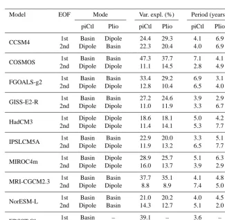
Table 3. Properties of empirical orthogonal functions (EOFs) of the Indian Ocean. The percentage of variance explained (var. expl.) by each model’s first two EOFs and the period with the most spectral power are shown. The correspondence of each EOF to physically meaningful modes of variability has been determined by visual inspection. The preindustrial and Pliocene simulations are denoted by piCtl and Plio, respectively.
Model EOF Mode Var. expl. (%) Period (years)
piCtl Plio piCtl Plio piCtl Plio
CCSM4 1st Basin Dipole 24.4 29.3 4.1 6.9 2nd Dipole Basin 22.3 20.4 4.0 6.9
COSMOS 1st Basin Basin 47.3 37.7 7.1 4.1 2nd Dipole Dipole 11.1 14.5 2.8 4.9
FGOALS-g2 1st Basin Basin 33.4 29.2 6.9 3.1 2nd Dipole Dipole 12.8 10.4 6.5 4.0
GISS-E2-R 1st Basin Basin 27.2 24.6 3.9 2.9 2nd Dipole Dipole 11.0 11.9 3.3 6.7
HadCM3 1st Dipole Dipole 18.6 18.1 5.0 4.2 2nd Dipole Dipole 11.4 14.1 5.3 7.7
IPSLCM5A 1st Basin Basin 22.9 20.0 3.3 5.1 2nd Dipole Dipole 11.9 13.2 6.5 7.7
MIROC4m 1st Basin Dipole 28.9 25.7 5.1 6.3 2nd Dipole Dipole 16.0 13.7 3.9 2.9
MRI-CGCM2.3 1st Basin Basin 37.7 35.1 4.1 4.8 2nd Dipole Dipole 8.8 8.9 7.4 5.0
NorESM-L 1st Basin Basin 21.0 20.2 4.0 4.5 2nd Dipole Basin 14.3 12.7 5.1 2.0
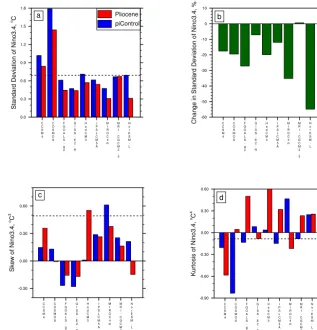
Figure 1. The moments of the distributions of the Niño 3.4 sea surface temperature anomalies in the ensemble members. The first moment (i.e. the mean) is 0 by definition. The standard deviation shows the amplitude of the SST variations. If the skew is positive, then the El Niño tail is stronger than the corresponding La Niña state. If the kurtosis is greater than 0, then the distribution is more peaked than a Gaussian. The dashed line shows the moment of the ERSST observations.
contribution from the 1.5-year low-pass filter applied here. These differences do lend a cautionary aspect as they high-light the centennial-scale variability in ENSO characteristics (Wittenberg, 2009) that could confound the results shown here.
The variance is the most discussed moment as it is a valu-able metric for the amplitude of the Niño 3.4 distribution. Here I will follow the conventional approach of presenting the standard deviation instead (e. g. Taschetto et al., 2014). There is a near unanimous weakening in ENSO amplitude seen in the mid-Pliocene simulations (Fig. 1a). The lone dis-senting model is MRI, which itself shows no change. The ensemble average standard deviation in the mid-Pliocene is only 80 % of the amplitude in the preindustrial control simu-lation (Fig. 1b; Table 2).
A less coherent pattern comes from looking at the higher moments of the distribution. It is observed that El Niños are generally stronger than their La Niña counterparts – equiva-lent to the Niño 3.4 distribution having a positive skew. This property is captured by two-thirds of the ensemble
mem-bers in the preindustrial conditions. However, the ensemble is equivocal about changes in skew for the Pliocene simula-tions (Fig. 1c). The kurtosis is a measure of spread of the dis-tribution compared to a Gaussian. A positive kurtosis means more of the activity occurs near the mean (0 by definition in this case) rather than out in the tails. Again there is little consistency across the ensemble as to the change in kurtosis (Fig. 1d).
or a reduction in kurtosis to alter the tail of the Niño 3.4 SST distribution such that more intense El Niños would be seen despite a reduction in variance overall.
3.1.2 Frequency
The only observational evidence of ENSO properties in the Pliocene relates to its frequency (Watanabe et al., 2012). Therefore, the simulated changes in the frequency are studied in isolation. This is achieved by normalising the time series by their standard deviations (Sect. 2.2). This then allows the individual power spectra to be averaged across the ensemble (Fig. 2). The power at the annual and sub-annual period have been removed through the data analysis (Sect. 2.2; unlike An and Choi, 2013).
Eight of the nine models show the dominant period of Niño 3.4 SSTA becoming longer; only COSMOS exhibits a shift to a shorter period (Table 2). This behaviour is also shown in the ensemble average power spectra (Fig. 2; see An and Choi, 2013, for discussion of this approach). Both these spectra exhibit two peaks at around 3 years and a stronger one at lower-frequencies. The lower frequency peak shifts substantially to longer periods; the significance of the smaller shift in the 3-year peak is debatable. A coherent lengthening of ENSO period is not robustly detected in future simula-tions. An and Choi (2013) notice a lengthening for the mid-Holocene, but only with the PMIP2 generation of models and not for PMIP3.
3.1.3 Structure
The conventional approach to investigate changes in the SST pattern associated with an El Niño involve compositing the events above a certain threshold (e.g. Haywood et al., 2007). I aim to study changes in the structure of climate variabil-ity patterns in isolation from any changes in amplitude or period, both of which show a robust Pliocene response indi-vidually. This is achieved by following the methodology of Power et al. (2013) through EOF analysis and normalisation. For each model, the first EOF of the tropical Pacific is sig-nificantly correlated to the Niño 3.4 (P <0.05 %). The first EOFs of the ensemble explain on average 60 % of the tropical Pacific variance in the preindustrial simulations compared to 56 % of the variance in the Pliocene simulations on the en-semble average.
The structure of ENSO is predominantly similar in the two time periods (Fig. 3). There is a shift towards the warmth of an El Niño expanding further across the tropical Pacific. Statistical significance with such a small ensemble is hard to compute (Sect. 4.3). Instead a simpler measure of co-herency is used – a location is considered coherent if more than seven of the nine models show a response in the same direction (Fig. 3). None of the individual models show sub-stantial changes in their ENSO structure (not shown).
Figure 2. The ensemble average power spectra of the Niño 3.4 sea surface temperature anomalies.
Figure 3. The ensemble average empirical orthogonal functions computed for the tropical Pacific. All patterns are defined to be pos-itive in the Niño 3.4 region (dotted line). Stippling indicates that less than eight of the nine models agree on the sign of the change. The change in standard deviation is defined as Pliocene minus preindus-trial.
3.1.4 Flavour
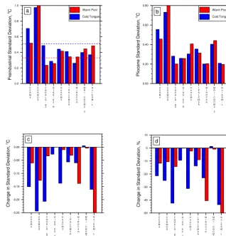
the cold-tongue and warm-pool types of ENSO show a large spread in quality of their simulation compared to observa-tions (Fig. 4a). This is also true of the wider CMIP5 ensem-ble (Taschetto et al., 2014).
The ensemble shows no robust change between the vari-ances of the two flavours (Fig. 4b–d). Instead the reduction in amplitude affects both flavours (only MRI-CGCM2 shows an increase in either form and even that is minimal). Both HadCM3 and NorESM-L switch the dominant flavour in the mid-Pliocene but in opposite directions. An alternate method to address the same question is to analyse the second EOF of the tropical Pacific. This also shows little coherent shift (not shown).
3.1.5 Summary
The PlioMIP ensemble is remarkable amongst climate en-sembles in that it shows a consistent message about changes in ENSO properties. ENSO in the Pliocene is simulated to have been weaker and less frequent. Changes in structure and flavour are less coherent, however. The reason why the PlioMIP ensemble shows a signal, whilst other ensembles do not, is unclear. Compared to CMIP5 future scenario en-sembles, this one has been run closer to equilibrium and has longer time series to analyse. However, that cannot be suf-ficient as other palaeoclimate ensembles do not see robust responses – for example, those of the mid-Holocene (An and Choi, 2013) and the Last Glacial Maximum (Zheng et al., 2007).
3.2 Tropical Indian variability
Climate variability in the tropical Indian Ocean has strong links to that in the Pacific, in part through their sharing of a single warm pool. The leading mode of Indian Ocean temperature variability is therefore a corollary to ENSO, al-though it is sometimes referred to as the Basin Mode (Deser et al., 2010). Around the turn of the century an additional mode of variability was identified – the Indian Ocean Dipole (IOD, Saji et al., 1999). The Indian Ocean Dipole can some-times track ENSO, yet it somesome-times operates in isolation. It manifests itself through changes in the zonal gradient of the Indian Ocean and can be tracked by the dipole mode index (Saji et al., 1999, DMI; Table 2). The quality of the preindus-trial simulation of the dipole mode index varies across the en-semble, as it does in the wider CMIP5 ensemble (Weller and Cai, 2013). Whilst several of the ensemble members show a change in amplitude of the Indian Ocean Dipole, there is no consensus in their sign (Table 2). The detection of a coher-ent signal may be hampered by biases in the climate models, meaning that the DMI is not capturing the centres of actions of the Indian Ocean Dipole.
An alternate approach is to use principal component anal-ysis to detect the Indian Ocean Dipole. A conventional methodology is to label the first EOF as the Basin Mode and
the second EOF as the Dipole Mode (Deser et al., 2010). Model biases mean this may not always be the correct; for example, both of the first two EOFs of HadCM3 show a basin-wide pattern. Therefore, visual inspection is used to categorise the nature of each the model-derived EOFs in comparison to those found from the detrended ERSST ob-servations. The results of this analysis are shown in Table 3, along with both the percentage variance explained by it and the dominant period of the accompanying principal compo-nent time series. It is hard to pull out a coherent message about Pliocene Indian Ocean variability from this ensemble, although it is interesting to note the potential for a change in the relative strengths of the two modes – as seen by CCSM4, for example (Table 3).
3.3 North Pacific variability
The dominant form of sea surface temperature variability in the North Pacific is a low-frequency mode termed the Pacific Decadal Oscillation (PDO, Mantua et al., 1997). The centre of action of this oscillation is the Kuroshio Extension around 40◦N, although it has significant impacts remote from this region. The connection between the PDO and low-frequency variations in ENSO is complex. Here, I follow Deser et al. (2010) and define the PDO as the first EOF of the North Pacific (20–70◦N). The EOF patterns are again normalised by their spatial standard deviations; however, in this instance both simulations are normalised by the preindustrial value. This retains information about the relative amplitude of the mode in the principal component time series. The standard deviations of the PDO time series are shown (Fig. 5a), along with the percentage change (Fig. 5b). There is little con-sistent response of the PDO amplitude to the imposing of the Pliocene conditions. The same is also true of the fre-quency and structure of the PDO when studied in isolation (not shown).
4 Discussion
Climate variability in three regions of the global ocean have been investigated in the PlioMIP ensemble. The nine con-stituent models often are equivocal about the changes in cli-mate variability that might have occurred in the Pliocene. However, for the two most studied facets of the domi-nant mode of variability, they provide a coherent message: Pliocene ENSO was weaker and less frequent.
This raises three questions: (a) how does this response fit the geological evidence; (b) can ENSO become so weak that it loses its global reach; and (c) what can explain the response of the PlioMIP ensemble?
4.1 Observations
Figure 4. Response of the two different flavours of ENSO considered separately. The flavours are disaggregated using the method of Ren and Jin (2011) into cold-tongue and warm-pool types. The red and blue dashed lines indicated the standard deviation found in the ERSST observations.
Figure 5. The standard deviations of Pacific Decadal Oscillation – defined as the first EOF of the North Pacific. The dashed line shows the standard deviation of the PDO in the ERSST observations.
Annular Mode, something not analysed here. Scroxton et al. (2011) use the distribution of single foraminifera in the east-ern equatorial Pacific to infer the presence of ENSO in the Pliocene. Changes in that distribution are more likely to reflect a response in the amplitude of the underlying
Pa-cific – in agreement with the results of Scroxton et al. (2011). However, it is doubtful that one would expect a lack of vari-ability in this region, even with a substantially reduced zonal SST gradient in the equatorial Pacific (Manucharyan and Fe-dorov, 2014).
The only other observational study of Pliocene climate variability looks at two fossil corals from the Philippines (Watanabe et al., 2012). Theδ18O is sampled at regular in-tervals during the corals’ roughly 30-year life span. A pe-riodicity of approximately 3 years is found in the Pliocene corals, which lived between 3.5 and 3.8 million years ago. This again provides evidence of ENSO variability in the trop-ical Pacific. Unfortunately, due to natural, internal shifts in ENSO properties on multidecadal timescales (Wittenberg, 2009), it would be impossible to infer an increase in this pe-riod with any confidence from the 30-year records available. 4.2 Global dominance
ENSO is the focus of substantial interest within the palaeocli-mate community, partly because it is the globally dominant mode of climate variability (Deser et al., 2010). It is projected to stay this way for the coming century (Christensen et al., 2013). In the PlioMIP ensemble, ENSO becomes weaker, whilst other modes of climate variability do not appear to do so. Is it possible that ENSO becomes so weak that its tele-connected response is not large enough to overwhelm local climate variability? Such a situation was suggested by Brier-ley (2013) as existing around 4 million years ago at the time of the weakest zonal SST gradients in the tropical Pacific (Fe-dorov et al., 2013).
Quantitatively detecting a change in global dominance is problematic. However, visual inspection of the leading global empirical orthogonal function can potentially show this. The two leading preindustrial EOFs of NorESM-L show strong signatures in both the North Pacific and the Niño region (Fig. 6a, b). In fact, their principal component time series show a marginally higher correlation with the PDO than ENSO – a feature not seen in observations. NorESM-L shows the strongest reduction in ENSO amplitude in the Pliocene across the ensemble (Table 2). For this model, the two lead-ing global EOFs in the Pliocene show no signature in the tropical Pacific (Fig. 6c, d). A similar feature is not seen with the other PlioMIP models (not shown).
Whilst this analysis does not state that ENSO in the Pliocene was confined to the tropical Pacific, it at least shows the potential for that to be the case. A lack of ENSO-style periodicities in regions remote from the tropical Pacific in the Pliocene may not denote a change in teleconnection pat-terns but, rather, be indicative of a weaker amplitude for ENSO. Attempts have been made to use present-day ENSO teleconnections to identify mean climate changes during the Pliocene (Molnar and Cane, 2007, 2002), although they have been dismissed as unconvincing (Bonham et al., 2009). That debate would further motivate an analysis of ENSO
telecon-nections in the PlioMIP ensemble. Unfortunately, sufficient temperature and precipitation data does not presently exist in the PlioMIP database to permit such an analysis across the ensemble.
4.3 (Statistical) Significance
The PlioMIP ensemble shows a weakening and lengthening of ENSO in the vast majority of the constituent models, but how significant is that? A thorough analysis of the statistical significance of even an individual model’s ENSO is a chal-lenge. I will obviously concentrate this discussion on ENSO, but the challenges are even larger for a lower-frequency os-cillation such as the PDO. Ideally, one would compare the Pliocene ENSO time series to multiple segments of a simi-lar length from the preindustrial control simulations. As the Pliocene time series here are 200 years long, a preindustrial control run of at least 10 times that is required to have suffi-cient segments. The longest preindustrial simulations readily available are only 1000 years (Saint-Lu et al., 2015). This means that there is insufficient data to create a probability distribution to test the possibility of drawing a segment with Pliocene-like ENSO properties. There are methods to esti-mate the probability without a very long control simulation (e. g. Stevenson et al., 2010). However, the interesting factor here is not whether each constituent model’s change may or may not be significant. Rather the surprising observation is the consistency across the ensemble in the reduction in am-plitude and frequency.
Other model ensembles show a range of behaviours and often contain more members than analysed here. So perhaps it is purely coincidental that the PlioMIP ensemble presents such a coherent message? Estimating the probability of a generic model ensemble showing a given level of coherence is problematic. A very simple approach is to consider each individual model having an equal chance of increase, reduc-tion or no change in an ENSO property (say, its amplitude). For eight out of nine ensemble members showing a similar change while the lone dissenter does not show an opposite response (as was found for both amplitude and period here), the probability is therefore
p(8 of 9)=2
3· 1
38 =0.000102. (2)
Figure 6. The first two EOFs of the global SST anomalies in NorESM-L for both the preindustrial simulation (left) and the Pliocene simulation (right). The percentage of the variance that each EOF explains is also shown.
with 7 decreasing and 2 with no change. The CMIP5 en-semble contains 27 models, with 8 decreasing and no change in 11 (Taschetto et al., 2014). There are 5071 combinations showing a reduction at least as robust as the PlioMIP ensem-ble out of a total 4.6×10⁶. This probability of only 0.01 % is likely somewhat of an underestimate because the lengths of simulation analysed by Taschetto et al. (2014) are substan-tially shorter than here (Stevenson et al., 2012). However, it does result in a similar estimate as above.
These calculations suggest that the PlioMIP signal did not occur by chance and is a real feature that needs exploring. Yet one must remember that many ensembles have been created and multiple ENSO properties have been investigated, which somewhat increases the likelihood of results like those seen in this particular ensemble occurring. One would be much more confident that the ENSO response described in Sect. 3.1 is a real future of the Pliocene climate if an underlying mech-anism could be found to explain them.
4.4 Physical mechanisms
There have been many suggestions as to what controls the properties of ENSO. It is beyond the scope of this article to test them all or to investigate the ENSO changes from a process-based approach. However, several possibilities can be easily evaluated from the data analysed here.
The commonality of PlioMIP experiments is in their appli-cation of (nearly) identical forcing and boundary condition changes (Haywood et al., 2011). The ENSO weakening and lengthening should therefore be a response to one of these boundary changes. Bonham (2011) investigated the response of ENSO in HadCM3. She found that changes in
topogra-phy represented the leading order determinant of the ENSO amplitude through a factor separation exercise (after Lunt et al., 2012). Confusingly, Bonham (2011) finds that topogra-phy leads to an increase in ENSO amplitude – potentially the use of a previous iteration of the PRISM topography is the explanation for this different signal. Feng and Poulsen (2014) find a response of ENSO to alterations in the elevation of the Andes mountain range, using CCSM4 simulations. The PRISM reconstruction has a lower Andes elevation in the Pliocene (Haywood et al., 2011). Unfortunately, Feng and Poulsen (2014) show that the Andes being lower would result in a shorter ENSO period – something that even the CCSM4 PlioMIP simulation does not show (Table 2). Therefore, any Andean response must be masked by another factor (assum-ing it is not model dependent, which is as yet untested).
ro-Figure 7. The annual mean Pacific temperature gradients along the Equator in the preindustrial simulations and the change in the Pliocene simulations.
bustly weaker and longer ENSO. There is a similar lack of explanation when assessing whether the mean state becomes more El Niño like (Fig. 8; Collins and The CMIP Modelling Groups, 2005).
An alternate possibility that can be easily tested is the sug-gestion that the amplitude of ENSO is inversely correlated to the seasonal amplitude (Liu, 2002). This possibility has already been questioned by Braconnot et al. (2011), and the PlioMIP ensemble does not show support for it either. Whilst there are changes in the seasonal cycle of Niño 3, they are not coherent across the PlioMIP ensemble (Fig. 9).
5 Conclusions
The Pliocene Model Intercomparison Project (PlioMIP) has coordinated nine coupled climate models to simulate the con-ditions of the mid-Piacenzian. Through analysis of sea sur-face temperature, I have described the interannual climate variability seen across the ensemble. Although some models show changes in the Indian Ocean Dipole or Pacific Decadal Oscillation, there was little coherency throughout the ensem-ble in these changes. Four different properties of the El Niño– Southern Oscillation have been isolated and the Pliocene changes in them investigated. There is no coherent change in the prevalence between the cold-tongue and warm-pool types of El Niño – in keeping with future projections (Taschetto et al., 2014). Analysis of the structure of ENSO finds a slight
Figure 8. A scatter plot of the change in ENSO amplitude (from Fig. 1) to the correlation of Pliocene mean state changes projected onto the model’s leading tropical Pacific EOF.
Figure 9. The seasonal cycle of the Niño 3 region average SST and its changes in the nine models.
expansion of the phenomenon further polewards – unlike the pattern found by Power et al. (2013) for the future projec-tions.
frequencies was unexpected. The chance of such a coher-ent message arising by chance is slim when considering the range of results in the CMIP5 future scenario runs (Taschetto et al., 2014). Three possible suggestions were investigated in the hope of explaining this result: namely reductions in the annual mean zonal temperature gradient (Fedorov and Phi-lander, 2001; Zhang et al., 2012b), Andean uplift (Feng and Poulsen, 2014) and seasonal cycle alterations. Until further investigation posits a viable physical mechanism behind this result, the possibility of it occurring by random chance can-not be satisfactorily dismissed, despite calculations suggest-ing it to be highly unlikely. Recent developments in process-based analysis (e.g. Jin et al., 2006) that are currently being applied to modern simulations (Bellenger et al., 2013) may help find the answer to this conundrum.
Acknowledgements. This work would not have been possible
without the cooperation of those modelling groups who submitted simulations to PlioMIP. I am especially grateful to (in alphabetical order) Pascale Braconnot, Fran Bragg, Wing-Le Chan, Mark Chandler, Camille Contoux, Aisling Dolan, Alan Haywood, Dan Hill, Youichi Kamae, Dan Lunt, Bette Otto-Bliesner, Jean-Yves Peterschmitt, Nan Rosenbloom, Linda Sohl, Christian Stepanek, Zhongshi Zhang and Weipeng Zheng. I would also like to further thank the PMIP Palaeovariability working group for their encour-agement.
Edited by: A. Haywood
References
An, S.-I. and Choi, J.: Mid-Holocene tropical Pacific climate state, annual cycle, and ENSO in PMIP2 and PMIP3, Clim. Dynam., 43, 1–14, doi:10.1007/s00382-013-1880-z, 2013.
Ashok, K., Behera, S. K., Rao, S. A., Weng, H., and Yamagata, T.: El Niño Modoki and its possible teleconnection, J. Geophys. Res., 112, C11007, doi:10.1029/2006JC003798, 2007.
Bellenger, H., Guilyardi, E., Leloup, J., Lengaigne, M., and Vialard, J.: ENSO representation in climate models: from CMIP3 to CMIP5, Clim. Dynam., 42, 1999–2018, doi:10.1007/s00382-013-1783-z, 2013.
Bonham, S. G.: Dynamics of Tropical Climate and High-Latitude Teleconnections during the Pliocene, PhD thesis, Univ. Leeds, UK, 2011.
Bonham, S. G., Haywood, A. M., Lunt, D. J., Collins, M., and Salzmann, U.: El Niño-Southern Oscillation, Pliocene cli-mate and equifinality, Philos. T. R. Soc. A, 367, 127–156, doi:10.1098/rsta.2008.0212, 2009.
Braconnot, P., Luan, Y., Brewer, S., and Zheng, W.: Impact of Earth’s orbit and freshwater fluxes on Holocene climate mean seasonal cycle and ENSO characteristics, Clim. Dynam., 38, 1081–1092, doi:10.1007/s00382-011-1029-x, 2011.
Bragg, F. J., Lunt, D. J., and Haywood, A. M.: Mid-Pliocene cli-mate modelled using the UK Hadley Centre Model: PlioMIP Experiments 1 and 2, Geosci. Model Dev., 5, 1109–1125, doi:10.5194/gmd-5-1109-2012, 2012.
Brierley, C.: ENSO behavior before the Pleistocene, PAGES news, 21, 70–71, 2013.
Brierley, C., Fedorov, A. V., Lui, Z., Herbert, T., Lawrence, K., and LaRiviere, J. P.: Greatly expanded tropical warm pool and weakened Hadley circulation in the early Pliocene, Science, 323, 1714–1718, doi:10.1126/science.1167625, 2009.
Cai, W., Zheng, X.-T., Weller, E., Collins, M., Cowan, T., Lengaigne, M., Yu, W., and Yamagata, T.: Projected response of the Indian Ocean Dipole to greenhouse warming, Nat. Geosci., 6, 999–1007, doi:10.1038/ngeo2009, 2013.
Cai, W., Borlace, S., Lengaigne, M., van Rensch, P., Collins, M., Vecchi, G. A., Timmermann, A., Santoso, A., McPhaden, M. J., Wu, L., England, M. H., Wang, G., Guilyardi, E., and Jin, F.-F.: Increasing frequency of extreme El Niño events due to greenhouse warming, Nature Climate Change, 4, 111–116, doi:10.1038/nclimate2100, 2014.
Chan, W.-L., Abe-Ouchi, A., and Ohgaito, R.: Simulating the mid-Pliocene climate with the MIROC general circulation model: experimental design and initial results, Geosci. Model Dev., 4, 1035–1049, doi:10.5194/gmd-4-1035-2011, 2011.
Chandler, M. A., Sohl, L. E., Jonas, J. A., Dowsett, H. J., and Kelley, M.: Simulations of the mid-Pliocene Warm Period using two ver-sions of the NASA/GISS ModelE2-R Coupled Model, Geosci. Model Dev., 6, 517–531, doi:10.5194/gmd-6-517-2013, 2013. Christensen, J. H., Krishna Kumar, K., Aldrian, E., An, S.-I.,
Cav-alcanti, I. F. A., de Castro, M., Dong, W., Goswami, B. N., Hall, A., Kanyanga, J. K., Kitoh, A., Kossin, J., Lau, N. C., Renwick, J., Stephenson, D. B., Xie, S.-P., and Zhou, T.: Climate phenom-ena and their relevance for future regional climate change, in: Climate Change 2013: The Physical Science Basis, edited by: Stocker, T. F., Dahe, Q., Plattner, G.-K., Tignor, M., Allen, S. K., Boschung, J., Nauels, A., Xia, Y., Bex, V., and Midgley, P. M., Cambridge University Press, Cambridge, UK and New York, NY, USA, 1217–1308, 2013.
Collins, M. and The CMIP Modelling Groups: El Niño- or La Niña-like climate change?, Clim. Dynam., 24, 89–104, doi:10.1007/s00382-004-0478-x, 2005.
Collins, M., An, S.-I., Cai, W., Ganachaud, A., Guilyardi, E., Jin, F.-F., Jochum, M., Lengaigne, M., Power, S., Timmermann, A., Vecchi, G. A., and Wittenberg, A. T.: The impact of global warm-ing on the tropical Pacific Ocean and El Niño, Nat. Geosci., 3, 391–397, doi:10.1038/ngeo868, 2010.
Collins, M., Knutti, R., Arblaster, J. M., Dufresne, J.-L., Fichefet, T., Friedlingstein, P., Gao, X., Gutowski, W. J., Johns, T. C., Krinner, G., Shongwe, M., Tebaldi, C., Weaver, A. J., and Wehner, M. F.: Long-term climate change: projections, commit-ments and irreversibility, in: Climate Change 2013: The Physical Science Basis, edited by: Stocker, T. F., Dahe, Q., Plattner, G.-K., Tignor, M., Allen, S. K., Boschung, J., Nauels, A., Xia, Y., Bex, V., and Midgley, P. M., Cambridge University Press, Cambridge, UK and New York, NY, USA, 1029–1136, 2013.
Contoux, C., Ramstein, G., and Jost, A.: Modelling the mid-Pliocene Warm Period climate with the IPSL coupled model and its atmospheric component LMDZ5A, Geosci. Model Dev., 5, 903–917, doi:10.5194/gmd-5-903-2012, 2012.
Dowsett, H. J., Robinson, M., Haywood, A. M., Salzmann, U., Hill, D. J., Sohl, L. E., Chandler, M., Williams, M., Foley, K. M., and Stoll, D. K.: The PRISM3D paleoenvironmental reconstruction, Stratigraphy, 7, 123–139, 2012.
Fedorov, A. V. and Philander, S. G.: A stability analysis of tropical ocean–atmosphere interactions: bridging measurements and the-ory for El Niño, J. Climate, 14, 3086–3101, doi:10.1175/1520-0442(2001)014<3086:ASAOTO>2.0.CO;2, 2001.
Fedorov, A. V., Dekens, P. S., McCarthy, M., Ravelo, A. C., de-Menocal, P. B., Barreiro, M., Pacanowski, R. C., and Philander, S. G.: The Pliocene paradox (mechanisms for a permanent El Niño), Science, 312, 1485–1489, doi:10.1126/science.1122666, 2006.
Fedorov, A. V., Brierley, C., and Emanuel, K. A.: Tropical cyclones and permanent El Niño in the early Pliocene epoch, Nature, 463, 1066–1070, doi:10.1038/nature08831, 2010.
Fedorov, A. V., Lawrence, K. T., Liu, Z., Dekens, P. S., Ravelo, A. C., and Brierley, C. M.: Patterns and mechanisms of early Pliocene warmth, Nature, 496, 43–49, doi:10.1038/nature12003, 2013.
Feng, R. and Poulsen, C. J.: Andean elevation control on tropi-cal Pacific climate and ENSO, Paleoceanography, 29, 795–809, doi:10.1002/2014PA002640, 2014.
Flato, G., Marotzke, J., Abiodun, B., Braconnot, P., Chou, S. C., Collins, W. J., Cox, P. M., Driouech, F., Emori, S., Eyring, V., Forest, C. E., Glecker, P. J., Guilyardi, E., Jakob, C., Kattsov, V. M., Reason, C. J. C., and Rummukainen, M.: Evaluation of climate models, in: Climate Change 2013: The Physical Science Basis, edited by: Stocker, T. F., Dahe, Q., Plattner, G.-K., Tignor, M., Allen, S. K., Boschung, J., Nauels, A., Xia, Y., Bex, V., and Midgley, P. M., Cambridge University Press, Cambridge, UK and New York, NY, USA, 741–866, 2013.
Haywood, A. M., Valdes, P. J., and Peck, V. L.: A permanent El Niño-like state during the Pliocene?, Paleoceanography, 22, PA1213, doi:10.1029/2006PA001323, 2007.
Haywood, A. M., Dowsett, H. J., Robinson, M. M., Stoll, D. K., Dolan, A. M., Lunt, D. J., Otto-Bliesner, B., and Chandler, M. A.: Pliocene Model Intercomparison Project (PlioMIP): experimen-tal design and boundary conditions (Experiment 2), Geosci. Model Dev., 4, 571–577, doi:10.5194/gmd-4-571-2011, 2011. Haywood, A. M., Hill, D. J., Dolan, A. M., Otto-Bliesner, B. L.,
Bragg, F., Chan, W.-L., Chandler, M. A., Contoux, C., Dowsett, H. J., Jost, A., Kamae, Y., Lohmann, G., Lunt, D. J., Abe-Ouchi, A., Pickering, S. J., Ramstein, G., Rosenbloom, N. A., Salz-mann, U., Sohl, L., Stepanek, C., Ueda, H., Yan, Q., and Zhang, Z.: Large-scale features of Pliocene climate: results from the Pliocene Model Intercomparison Project, Clim. Past, 9, 191–209, doi:10.5194/cp-9-191-2013, 2013.
Hill, D. J., Csank, A. Z., Dolan, A. M., and Lunt, D. J.: Pliocene climate variability: Northern Annular Mode in mod-els and tree-ring data, Palaeogeogr. Palaeocl., 309, 118–127, doi:10.1016/j.palaeo.2011.04.003, 2011.
Jin, F.-F., Kim, S. T., and Bejarano, L.: A coupled-stability index for ENSO, Geophys. Res. Lett., 33, L23708, doi:10.1029/2006GL027221, 2006.
Kamae, Y. and Ueda, H.: Mid-Pliocene global climate simula-tion with MRI-CGCM2.3: set-up and initial results of PlioMIP Experiments 1 and 2, Geosci. Model Dev., 5, 793–808, doi:10.5194/gmd-5-793-2012, 2012.
Knutson, T. R., McBride, J. L., Chan, J., Emanuel, K. A., Holland, G., Landsea, C., Held, I. M., Kossin, J. P., Srivastava, A. K., and Sugi, M.: Tropical cyclones and climate change, Nat. Geosci., 3, 157–163, doi:10.1038/ngeo779, 2010.
Liu, J.: Mechanism study of the ENSO and southern high lat-itude climate teleconnections, Geophys. Res. Lett., 29, 1679, doi:10.1029/2002GL015143, 2002.
Lunt, D. J., Haywood, A. M., Schmidt, G. A., Salzmann, U., Valdes, P. J., Dowsett, H. J., and Loptson, C. A.: On the causes of mid-Pliocene warmth and polar amplification, Earth Planet. Sc. Lett., 321–322, 128–138, doi:10.1016/j.epsl.2011.12.042, 2012. Mantua, N. J., Hare, S. R., Zhang, Y., Wallace, J. M., and Francis,
R. C.: A Pacific interdecadal climate oscillation with impacts on salmon production, B. Am. Meteorol. Soc., 78, 1069–1079, doi:10.1175/1520-0477(1997)078<1069:APICOW>2.0.CO;2, 1997.
Manucharyan, G. E. and Fedorov, A. V.: Robust ENSO across a Wide Range of Climates, J. Climate, 27, 5836–5850, doi:10.1175/JCLI-D-13-00759.1, 2014.
Masson-Delmotte, V., Schulz, M., Abe-Ouchi, A., Beer, J., Ganopolski, A., Gonzalez Rouco, J. F., Jansen, E., Lambeck, K., Luterbacher, J., Naish, T., Osborn, T. J., Otto-Bliesner, B., Quinn, T. M., Ramesh, R., Rojas, M., Shao, X., and Timmermann, A.: Information from paleoclimate archives, in: Climate Change 2013: The Physical Science Basis, edited by: Stocker, T. F., Dahe, Q., Plattner, G.-K., Tignor, M., Allen, S. K., Boschung, J., Nauels, A., Xia, Y., Bex, V., and Midgley, P. M., Cambridge University Press, Cambridge, UK and New York, NY, USA, 383– 464, 2013.
Molnar, P. H. and Cane, M. A.: El Niño’s tropical climate and teleconnections as a blueprint for pre-Ice Age climates, Paleo-ceanography, 17, 1021, doi:10.1029/2001PA000663, 2002. Molnar, P. H. and Cane, M. A.: Early Pliocene (pre-Ice Age) El
Niño–like global climate: Which El Niño?, Geosphere, 3, 337– 365, doi:10.1130/GES00103.1, 2007.
Power, S., Delage, F., Chung, C., Kociuba, G., and Keay, K.: Robust twenty-first-century projections of El Niño and related precipita-tion variability, Nature, 502, 541–545, doi:10.1038/nature12580, 2013.
Ren, H.-L. and Jin, F.-F.: Niño indices for two types of ENSO, Geo-phys. Res. Lett., 38, L04704, doi:10.1029/2010GL046031, 2011. Rosenbloom, N. A., Otto-Bliesner, B. L., Brady, E. C., and Lawrence, P. J.: Simulating the mid-Pliocene Warm Period with the CCSM4 model, Geosci. Model Dev., 6, 549–561, doi:10.5194/gmd-6-549-2013, 2013.
Saint-Lu, M., Braconnot, P., Leloup, J., Lengaigne, M., and Marti, O.: Changes in the ENSO/SPCZ relationship from past to future climates, Earth Planet. Sc. Lett., 412, 18–24, doi:10.1016/j.epsl.2014.12.033, 2015.
Saji, N. H., Goswami, B. N., Vinayachandran, P. N., and Yamagata, T.: A dipole mode in the tropical Indian Ocean, Nature, 401, 360– 363, doi:10.1038/43854, 1999.
Scroxton, N., Bonham, S. G., Rickaby, R. E. M., Lawrence, S. H. F., Hermoso, M., and Haywood, A. M.: Persistent El Niño-Southern oscillation variation during the Pliocene epoch, Paleoceanogra-phy, 26, PA2215, doi:10.1029/2010PA002097, 2011.
temperature analysis (1880–2006), J. Climate, 21, 2283–2296, doi:10.1175/2007JCLI2100.1, 2008.
Stepanek, C. and Lohmann, G.: Modelling mid-Pliocene cli-mate with COSMOS, Geosci. Model Dev., 5, 1221–1243, doi:10.5194/gmd-5-1221-2012, 2012.
Stevenson, S., Fox-Kemper, B., Jochum, M., Rajagopalan, B., and Yeager, S.: ENSO Model Validation Using Wavelet Probability Analysis, J. Climate, 22, 5540–5547, doi:10.1175/2010JCLI3609.1, 2010.
Stevenson, S., Fox-Kemper, B., Jochum, M., Neale, R. B., Deser, C., and Meehl, G.: Will there be a significant change to El Niño in the twenty-first century?, J. Climate, 25, 2129–2145, doi:10.1175/JCLI-D-11-00252.1, 2012.
Taschetto, A. S., Gupta, A. S., Jourdain, N. C., Santoso, A., Ummenhofer, C. C., and England, M. H.: Cold tongue and warm pool ENSO events in CMIP5: mean state and future pro-jections, J. Climate, 27, 2861–2885, doi:10.1175/JCLI-D-13-00437.1, 2014.
Thirumalai, K., Partin, J. W., Jackson, C. S., and Quinn, T. M.: Sta-tistical constraints on El Niño Southern Oscillation reconstruc-tions using individual foraminifera: a sensitivity analysis, Paleo-ceanography, 28, 401–412, doi:10.1002/palo.20037, 2013. Trenberth, K. E.: The definition of El Niño, B. Am.
Meteorol. Soc., 78, 2771–2777, doi:10.1175/1520-0477(1997)078<2771:TDOENO>2.0.CO;2, 1997.
UCAR: The NCAR Command Language, doi:10.5065/D6WD3XH5, available at:
http://www.ncl.ucar.edu/, last access: 8 February 2015, 2014. von der Heydt, A. S., Nnafie, A., and Dijkstra, H. A.: Cold
tongue/Warm pool and ENSO dynamics in the Pliocene, Clim. Past, 7, 903–915, doi:10.5194/cp-7-903-2011, 2011.
Wara, M. W., Ravelo, A. C., and Delaney, M. L.: Permanent El Niño-like conditions during the Pliocene warm period, Science, 309, 758–761, 2005.
Watanabe, T., Suzuki, A., Minobe, S., Kawashima, T., Kameo, K., Minoshima, K., Aguilar, Y. M., Wani, R., Kawahata, H., Sowa, K., Nagai, T., and Kase, T.: Permanent El Niño during the Pliocene warm period not supported by coral evidence, Nature, 471, 209–211, doi:10.1038/nature09777, 2012.
Weller, E. and Cai, W.: Realism of the Indian Ocean dipole in CMIP5 models: the implications for climate projections, J. Cli-mate, 26, 6649–6659, doi:10.1175/JCLI-D-12-00807.1, 2013. Wittenberg, A. T.: Are historical records sufficient to
con-strain ENSO simulations?, Geophys. Res. Lett., 36, L12702, doi:10.1029/2009GL038710, 2009.
Zhang, Z. S., Nisancioglu, K., Bentsen, M., Tjiputra, J., Bethke, I., Yan, Q., Risebrobakken, B., Andersson, C., and Jansen, E.: Pre-industrial and mid-Pliocene simulations with NorESM-L, Geosci. Model Dev., 5, 523–533, doi:10.5194/gmd-5-523-2012, 2012a.
Zhang, Z., Yan, Q., and Su, J. Z.: Has the problem of a permanent El Niño been resolved for the mid-Pliocene, Atmospheric and Oceanic Science Letters, 5, 445–448, 2012b.
Zheng, W., Braconnot, P., Guilyardi, E., Merkel, U., and Yu, Y.: ENSO at 6 ka and 21 ka from ocean–atmosphere coupled model simulations, Clim. Dynam., 30, 745–762, doi:10.1007/s00382-007-0320-3, 2007.