www.nonlin-processes-geophys.net/22/749/2015/ doi:10.5194/npg-22-749-2015
© Author(s) 2015. CC Attribution 3.0 License.
Nonlinear feedback in a six-dimensional Lorenz model:
impact of an additional heating term
B.-W. Shen
Department of Mathematics and Statistics, San Diego State University, 5500 Campanile Drive, San Diego, CA 92182-7720, USA
Correspondence to: B.-W. Shen ([email protected], [email protected])
Received: 20 February 2015 – Published in Nonlin. Processes Geophys. Discuss.: 17 March 2015 Revised: 15 October 2015 – Accepted: 2 December 2015 – Published: 21 December 2015
Abstract. In this study, a six-dimensional Lorenz model (6DLM) is derived, based on a recent study using a five-dimensional (5-D) Lorenz model (LM), in order to exam-ine the impact of an additional mode and its accompanying heating term on solution stability. The new mode added to improve the representation of the streamfunction is referred to as a secondary streamfunction mode, while the two addi-tional modes, which appear in both the 6DLM and 5DLM but not in the original LM, are referred to as secondary temper-ature modes. Two energy conservation relationships of the 6DLM are first derived in the dissipationless limit. The im-pact of three additional modes on solution stability is exam-ined by comparing numerical solutions and ensemble Lya-punov exponents of the 6DLM and 5DLM as well as the orig-inal LM. For the onset of chaos, the critical value of the nor-malized Rayleigh number (rc) is determined to be 41.1. The critical value is larger than that in the 3DLM (rc∼24.74), but slightly smaller than the one in the 5DLM (rc∼42.9). A stability analysis and numerical experiments obtained us-ing generalized LMs, with or without simplifications, sug-gest the following: (1) negative nonlinear feedback in asso-ciation with the secondary temperature modes, as first iden-tified using the 5DLM, plays a dominant role in providing feedback for improving the solution’s stability of the 6DLM, (2) the additional heating term in association with the sec-ondary streamfunction mode may destabilize the solution, and (3) overall feedback due to the secondary streamfunc-tion mode is much smaller than the feedback due to the sec-ondary temperature modes; therefore, the critical Rayleigh number of the 6DLM is comparable to that of the 5DLM. The 5DLM and 6DLM collectively suggest different roles for small-scale processes (i.e., stabilization vs. destabilization),
consistent with the following statement by Lorenz (1972): “If the flap of a butterfly’s wings can be instrumental in generat-ing a tornado, it can equally well be instrumental in prevent-ing a tornado.” The implications of this and previous work, as well as future work, are also discussed.
1 Introduction
Fifty years have passed since Lorenz published his break-through modeling study (Lorenz, 1963) that changed our view regarding the predictability of weather and climate (e.g., IPCC, 2007; Pielke, 2008), laying the foundation for chaos theory (e.g., Gleick, 1987; Anthes, 2011). Since the degree of nonlinearity is finite in the original Lorenz model referred to as 3DLM, the impact of increased nonlinearity on systems’ solutions and/or their stability has been stud-ied using generalized Lorenz models (LMs) with additional Fourier modes (e.g., Curry, 1978; Curry et al., 1984; Frances-chini and Tebaldi, 1985; Howard and Krishnamurti, 1986; Franceschini et al., 1988; Hermiz et al., 1995; Thiffeault and Horton, 1996; Musielak et al., 2005; Chen and Price, 2006; Roy and Musielak, 2007a, b, c; Lucarini and Fraedrich, 2009). However, such studies do not provide a definite an-swer regarding whether or not higher-order LMs lead to more stable solutions.
3DLM was defined by Shen14 as a pair of downscale and upscale transfer processes associated with the Jacobian func-tion (in Eq. 2). The feedback loop has been suggested to sta-bilize the solution for 1< r <24.74 within the 3DLM, as compared to the linearized 3DLM. Extending the nonlinear feedback loop in a five-dimensional LM (5DLM) can pro-vide negative nonlinear feedback to produce non-trivial sta-ble critical points when 1< r <42.9. The negative nonlinear feedback represents the collective impact of additional non-linear terms and dissipative terms introduced by the two ad-ditional Fourier modes of the 5DLM. In this study (and in the previous study, Shen14), the two modes are added to improve the representation of the temperature perturbation, referred to here as secondary temperature modes. Improved stability with a higher critical Rayleigh parameter was verified by lin-earizing the 5DLM with respect to a non-trivial critical point and then performing a stability analysis over a wide range of values in parameters (σ,r). The outcome was possible due to the analytical solutions of the critical points in the 5DLM (e.g., Shen14). The role of the negative nonlinear feedback was further verified using the revised 3DLM that parame-terizes the negative nonlinear feedback to suppress chaotic responses using a nonlinear eddy dissipation term.
In addition to the negative nonlinear feedback, Shen14 indicated that a conclusion derived from lower-dimensional LMs may not be applicable in all circumstances in a higher-dimensional LM. For example, although the butterfly effect (of the first kind) with dependence of solutions on initial conditions appears in the 3DLM within the range between r=25 and 40, it does not exist in the 5DLM. Therefore, to examine whether or not small perturbations can alter large-scale structure (i.e., the butterfly effect of the second kind), a model containing proper representations of multiscale pro-cesses and their nonlinear interactions is required. As a re-sult, it would require improving the degree of nonlinearity to address the question.
In a pioneering study using the generalized LM with a large number of Fourier modes, Curry et al. (1984) sug-gested that chaotic responses disappeared when sufficient modes were included. Shen14 hypothesized that the system’s stability in the LMs, with a finite number of modes, can be improved with additional modes that provide negative non-linear feedback associated with additional dissipative terms. However, since new modes can also introduce additional heating term(s), the competing role of the heating term(s) with nonlinear terms and/or with dissipative terms deserves to be examined so that the conditions under which solutions become more stable or chaotic can be better understood. Re-sults obtained from work described here and the work of Shen14 are used to address the following question: for gener-alized LMs, under which conditions can the increased degree of nonlinearity improve solution stability?
To achieve the goal outlined above, the 3DLM to 5DLM was previously extended in Shen14 by including the two sec-ondary temperature modes. In this study, the 5DLM is
ex-tended to the 6DLM by adding an additional mode. The ad-ditional mode is included to improve the representation of the streamfunction (e.g., Eqs. 4 and 5), and is, therefore, re-ferred to as the secondary streamfunction mode. While the secondary temperature modes of the 5DLM (as well as the 6DLM) introduce additional nonlinear terms and dissipative terms, which, in turn, provide negative nonlinear feedback, the secondary streamfunction mode of the 6DLM introduces additional nonlinear terms and adds a heating term. The ap-proach, using incremental changes in the number of Fourier modes, can help trace their individual and/or collective im-pact on solution stability. For example, since the 6DLM also contains the negative nonlinear feedback in association with secondary temperature modes, it becomes feasible to exam-ine the role of the additional heating term in the solution’s stability and its competing impact with the negative nonlin-ear feedback.
The presented work is organized as follows. We describe the governing equations in Sect. 2.1 and present the deriva-tions of the 6DLM in Sect. 2.2. We then discuss the en-ergy conservation of the 6DLM in the dissipationless limit in Sect. 2.3, and numerical approaches for integrations of the LMs and calculations of ensemble Lyapunov exponents in Sect. 2.4. In Sect. 3.1, we investigate the potential impact of the additional heating term on the solution’s stability by performing stability analysis near the trivial critical point. We also illustrate how the feedback loop can be extended using the secondary streamfunction mode. In Sect. 3.2, nu-merical results obtained from the 6DLM are provided and compared to results obtained from the 5DLM. To examine the role of the secondary streamfunction mode and to iden-tify the major nonlinear feedback term, additional numeri-cal experiments using the 6DLM and simplified 6DLMs are compared in Sect. 3.3. Then, we discuss the dependence of the solution’s stability on the Prandtl number (σ) in Sect. 3.4. Concluding remarks appear at the end. Mathematical deriva-tions of the 5DLM and 6DLM are briefly summarized in the Supplement.
2 The six-dimensional Lorenz model and numerical methods
2.1 The governing equations
By assuming 2-D (x, z), incompressible and Boussinesq flow, the following equations were used by Saltzman (1962) and Lorenz (1963):
∂ ∂t∇
2ψ= −Jψ,∇2ψ+ν∇4ψ+gα∂θ
∂x, (1)
∂θ
∂t = −J (ψ, θ )+ 1T
H ∂ψ ∂x +κ∇
2θ. (2)
vertical velocities;θis the temperature perturbation; and1T represents the temperature difference at the bottom and top boundaries. The constantsg,α,ν, andκ denote the accel-eration of gravity, the coefficient of thermal expansion, the kinematic viscosity, and the thermal conductivity, respec-tively. The Jacobian of two arbitrary functions is defined as J (A, B)=(∂A/∂x) (∂B/∂z)−(∂A/∂z) (∂B/∂x). Addition-ally,
∇4ψ=∂/∂x∇2∂ψ/∂x+∂/∂z∇2∂ψ/∂z.
Based on the above partial differential equations, Lorenz (1963) introduced a system of three ordinary differential equations to illustrate the characteristics of chaotic solutions. This system is a simplified version of the one derived by Saltzman (1962). For the reader’s convenience, the same symbols as those in Saltzman (1962) and Lorenz (1963) are used here.
2.2 The 6-D Lorenz model (6DLM)
To generalize the original Lorenz model, we first use the fol-lowing six Fourier modes (which are also listed in Table 1 of Shen14) to derive the 6DLM:
M1= √
2 sin(lx)sin(mz), M2= √
2 cos(lx)sin(mz),
M3=sin(2mz), (3)
M4= √
2 sin(lx)sin(3mz), M5= √
2 cos(lx)sin(3mz),
M6=sin(4mz). (4)
Here l andmare defined asπ a/H andπ/H, representing the horizontal and vertical wavenumbers, respectively, and a is a ratio of the vertical scale of the convection cell to its horizontal scale, i.e., a=l/m. The term H is the domain height, and 2H /arepresents the domain width. Using these modes,ψandθcan be represented as follows:
ψ=C1(XM1+X1M4), (5)
θ=C2(Y M2+Y1M5−ZM3−Z1M6) , (6) C1=κ
(1+a2) a , C2=
1T π
Rc Ra
, Rc= π4 a2(1+a
2)3,
Ra−1= νκ gαH31T,
whereC1andC2are constants, Ra is the Rayleigh number andRcis its critical value for the free-slip Rayleigh–Benard problem. Using Eqs. (5) and (6), solutions within the 6DLM are represented by the six spatial modesM1toM6(Eqs. 3, 4) and their corresponding time-varying amplitudes (X,Y, Z, X1, Y1, Z1), respectively. By comparison, Eq. (3) was used to derived the 3DLM, and Eqs. (3) and (4) withoutM4 were used to derive the 5DLM. While the 3DLM and 6DLM (5DLM) have one horizontal wavenumber, they contain two and four vertical wavenumbers, respectively. In the text be-low, to facilitate discussions, M1 andM4are referred to as
primary and secondary streamfunction modes, respectively, M2 andM3are referred to as primary temperature modes, and M5 and M6 are referred to as secondary temperature modes. Here, the reader should note that an implicit limi-tation of this approach is that nonlinear interactions among the selected modes cannot generate (impact) any new (other) modes that are not pre-selected, suggesting limited (spatial) scale interactions. While the impact of the secondary tem-perature modes (i.e.,Y1 andZ1) on the solution’s stability was discussed by Shen14 with the 5DLM, the impact of the secondary streamfunction mode (i.e.,X1), which introduces a heating term (rX1), is the focus of the 6DLM provided here.
To transform Eqs. (1) and (2) into the “phase” space, a ma-jor step is to calculate the nonlinear Jacobin functions. Cal-culations indicate that J (ψ,∇2ψ )in Eq. (1) does not lead to any explicit term in the final 6DLM, or the 3DLM or the 5DLM. Here, the Jacobian term of Eq. (2), which is written as follows, is discussed:
J (ψ, θ )=C1C2(XY J (M1, M2)−XZJ (M1, M3) +XY1J (M1, M5)−XZ1J (M1, M6) +X1Y J (M4, M2)−X1ZJ (M4, M3)
+X1Y1J (M4, M5)−X1Z1J (M4, M6)). (7) Note that the 3DLM only contains the first two terms on the right-hand side of Eq. (7), namely XY J (M1, M2) and −XZJ (M1, M3), while the 5DLM includes the first four terms.
After derivations, we obtain the 6DLM with the following six equations:
dX
dτ = −σ X+σ Y, (8)
dY
dτ = −XZ+X1Z−2X1Z1+rX−Y, (9) dZ
dτ =XY−XY1−X1Y−bZ, (10)
dX1
dτ = −doσ X1+ σ do
Y1, (11)
dY1
dτ =XZ−2XZ1+rX1−doY1, (12) dZ1
The 3DLM can be obtained from the 6DLM when terms that involve (X1,Y1,Z1) are neglected. Alternatively, Eqs. (8)–(10) can be viewed as a 3DLM with the feedback processes that result from the three additional modes. There-fore, the 6DLM can be viewed as a coupled system that con-sists of the 3DLM (Eqs. 8–10) and a forced dissipative sys-tem with an additional heating term (e.g., Eqs. 11–13). Here, and in Shen14, unless otherwise stated, the term “feedback” refers to the nonlinear process that involves the secondary modes, namely (X1,Y1, and/orZ1). The 5DLM in Shen14 can be also obtained by ignoring theX1and dX1/dτ in the 6DLM. As a result, the 6DLM can be viewed as a coupled system that consists of the 5DLM and an additional equation (i.e., Eq. 11) that introduces nonlinear feedback associated with an additional heating term (i.e., Eq. 12).
2.3 Energy conservation in the 6-D non-dissipative LM The domain-averaged kinetic energy (KE), available poten-tial energy (APE), and potenpoten-tial energy (PE) are defined (e.g., Treve and Manley, 1982; Thiffeault and Horton, 1996; Blender and Lucarini, 2013; Shen, 2014a), as follows:
KE=1
2 2H /a
Z
0
H
Z
0
(u2+w2)dzdx, (14)
APE= −gαH
21T 2H /a
Z
0
H
Z
0
(θ )2dzdx, (15)
PE= − 2H /a
Z
0
H
Z
0
gα(zθ )dzdx. (16)
Through straightforward derivations, we obtain the following equations:
KE=Co
2 (X 2+d
oX21), (17a)
KEp= Co
2 X
2. (17b)
HereCo=π2κ2
1+a2 a
3
. KEpcontains only a portion of the total KE of the 6DLM from the primary streamfunction mode X, but represents the total KE in the 5DLM and 3DLM. In a similar manner, as follows,
APE= −Co
2 σ
r(Y
2+Z2+Y2 1+Z
2
1), (18)
PE= −Coσ (Z+Z1/2). (19)
Equations (17a) and (18) yield the following: KE+APE=Co
2
X2+doX21−
σ
r
Y2+Z2+Y12+Z21
=C3, (20)
while Eqs. (17b) and (19) lead to the following:
KEp+PE=Co
X2
2 −σ
Z+Z1
2
!
=C4. (21)
With Eqs. (8)–(13) in the dissipationless limit, the time derivatives of both Eqs. (20) and (21) are zero, so bothC3 andC4are constants. Therefore, Eqs. (20) and (21) indicate two energy conservation laws, including the conservation of the total KE and APE (i.e., Eq. 20). However, it should be noted that, as follows,
KE+PE=Co
X2
2 +do
X21
2 −σ
Z+Z1
2
!
6=constant. (22)
By comparison, the two energy conservation laws of the 5DLM are written as follows:
KE5-D+APE5-D=
Co
2
X2−σ r
Y2+Z2+Y12+Z12=C5, (23)
KE5-D+PE5-D=Co X2
2 −σ
Z+Z1
2
=C6. (24) It can been shown that bothC5andC6are constants. There-fore, in the 5DLM, in addition to the conservation of the KE and APE, the KE and PE are also conserved.
2.4 Numerical approaches
Using the fourth-order Runge–Kutta scheme, the original and higher-order Lorenz models are integrated forward in time. We vary the value of the heating parameterrbut keep other parameters as constants, including σ=10,a=1/
√
2,b=
8/3,do=19/3, and a minimum value forRc=27π4/4. In Figs. 1, 2, 3 and 6, the initial conditions are given as follows: (X, Y, Z, X1, Y1, Z1)=(0,1,0,0,0,0). (25) The dimensionless time interval (4τ) is 0.0001. The total number of time steps (N) is 1 000 000 in Fig. 1 and 500 000 in Figs. 2, 3, and 6, yielding a total dimensionless time (τ) of 100 and 50, respectively. In Figs. 2 and 6, the solutions of the 3DLM and 5DLM are rescaled by the analytical solutions of their critical points (i.e., Eqs. 21 and 19 of Shen14). The solutions of the 6DLM are rescaled by the critical points of the 5DLM. In Sect. 3.4, the dependence of solution stability on the Prandtl number (σ) is discussed with selected values ofσ.
0 20 40 60 80 100
−0.10
−0.05
0.00
0.05
0.10
KE+APE and KE+PE (r=25)
Time (tau) KE+APE−IC+0.0 (5D−NLM) KE+APE−IC+0.02 (6D−NLM) KE+PE−IC+0.04 (5D−NLM) KEp+PE−IC+0.06 (6D−NLM) (a)
0 20 40 60 80 100
−0.10
−0.05
0.00
0.05
0.10
KE+APE and KE+PE (r=45)
Time (tau) KE+APE−IC+0.0 (5D−NLM) KE+APE−IC+0.02 (6D−NLM) KE+PE−IC+0.04 (5D−NLM) KEp+PE−IC+0.06 (6D−NLM) (b)
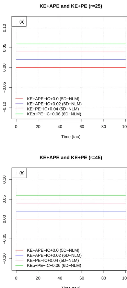
Figure 1. Time evolution of energy conservation laws from the
5D-NLM and 6D-5D-NLM. (KE+PE) and (KE+APE) are displayed for
the 5D-NLM, while (KEp+PE) and (KE+APE) are shown for the
6D-NLM. (a) and (b) are forr=25 andr=45, respectively. All
fields are normalized using the constant Co
=π2κ21+aa23
,
and each of the above lines is shifted to the summation of the cor-responding initial value and a constant value (e.g., 0.06 in the green line).
and Ding, 2011). In Shen14, the two methods implemented and tested are the trajectory separation (TS) method (e.g., Sprott, 1997, 2003); and the Gram–Schmidt reorthonormal-ization (GSR) procedure (e.g., Wolf et al., 1985; Christiansen
and Rugh, 1997). Here, a brief summary of how LEs are cal-culated using the two methods is provided. Using given ini-tial conditions (ICs) and a set of parameters in the LMs, the TS scheme calculates the largest LE, and the GSR scheme produces “n” LEs; here “n” is the dimension of the 5-D or 6-D LM. Calculations are conducted with4τ =0.0001 andN=10 000 000, yieldingτ =1000. To minimize the de-pendence on the ICs, 10 000 ensemble (En=10 000) runs with the same model configurations but different ICs are performed, and an ensemble averaged LE (eLE) is obtained from the average of the 10 000 LEs. A largeN and En are used to understand the long-term average behavior of the so-lutions of the LMs and simplified LMs where some terms are ignored. While eLEs calculations using the above two methods were previously discussed and compared in Shen14, here, a calculation of the Kaplan–Yorke fractal dimension (Kaplan and Yorke, 1979) using the (three) leading eLEs from the GSR method is provided in Appendix A as an addi-tional verification. Unless stated otherwise in the main text, the largest ensemble-averaged LE (eLE) for a givenris ob-tained from the TS method.
To examine the collective or individual impact of the non-linear feedback terms and to identify the major feedback that can improve numerical predictability in the 5-D and 6-D LMs, we perform additional runs using the 6DLM with addi-tional simplifications. The experiments, as listed in Table 1, include the following: (1) case 6DLMS1 where three nonlin-ear terms involvingX1are neglected and only one feedback term (XY1) is retained in Eqs. (9) and (10), (2) case 6DLMS2 where onlyXY1is ignored in Eq. (10), and (3) case 6DLMS3 whererX1is removed from Eq. (12). Results from these sim-plified 6DLMs are presented in Sect. 3.3.
3 Discussion
In the following sections, we discuss the impact of additional modes on solution stability. In Sect. 3.1, we illustrate the po-tential role of theM4 mode by performing linear stability analysis at the trivial critical point. In Sects. 3.2 and 3.3, we present and compare numerical results from the 6DLM with and without simplifications to identify the major feedback process. The dependence of solution stability on the Prandtl number (σ) is discussed in Sect. 3.4.
3.1 The impact ofM4on linear stability
Table 1. A list of numerical experiments for different Lorenz models. The column “Modifications” indicates additional changes in the “Equations”. Thercandrclare determined based on the eLE analyses and the linear stability analysis, respectively. Solutions in “Figures” are
rescaled using the factors listed in the “Scaling factors”.∗For the 3DLM, the ensemble averaged LE is 1.2×10⁻²atr=23.7, and becomes
0.26 atr=24. The 5-D and 6-D non-dissipative Lorenz models (5D-NLM and 6D-NLM) are used to examine the energy conservation
properties.
Case IDs Equations Modifications Figures rc rcl Scaling factors
3DLM Eqs. (15)–(17) of Shen14 N/A 2 23.7∗ 24.74 Eq. (21) of Shen14
5DLM Eqs. (10)–(14) of Shen14 N/A 2–5, 7 42.9 45.94 Eq. (19) of Shen14
6DLM Eqs. (8)–(13) N/A 2–7 41.1 N/A Same
6DLMS1 Eqs. (8)–(13) Ignoring terms that involveX1in Eqs. (9) and (10) 5, 6 42.3 N/A Same
6DLMS2 Eqs. (8)–(13) Ignoring the term−XY1in Eq. (10) 5, 6 23.9 N/A Same
6DLMS3 Eqs. (8)–(13) Ignoring the termrX1in Eq. (12) 5, 6 42.1 N/A Same
5D-NLM Eqs. (10)–(14) of Shen14 Ignoring dissipative terms 1 N/A N/A N/A
6D-NLM Eqs. (8)–(13) Ignoring dissipative terms 1 N/A N/A N/A
4T ∂ψ/∂xof Eq. (2) provides feedback to theM5mode (in Table 1 of Shen14). TheM4mode shares the same horizon-tal and vertical wavenumbers as theM5, but has a different phase (i.e., sin(lx)vs. cos(lx)in Eq. 4). Alternatively, via the ∂θ/∂x and4T ∂ψ/∂x, theM4andM5modes are linked as follows:
dX1
dτ ∝ −doσ X1+ σ do
Y1, (26)
dY1
dτ ∝rX1−doY1, (27)
which can be derived by linearizing Eqs. (11) and (12) at the trivial critical point. The linearized equations are decoupled with the rest of the equations on the 6DLM, suggesting that the heating term (rX1) can impact other modes as well as the stability of the nonlinear 6DLM via nonlinear feedback, as discussed below. The above equations are reduced to the following:
d2Y1
dτ2 +do(σ+1) dY1
dτ − σ do
r−do3=0. (28)
By assuming the solution Y1∝exp(βτ ), we obtain the fol-lowing two roots forβ:
β±(r)=
−do(σ+1)±
r
do2(σ+1)2+4σ
r−do3
/do
2 . (29)
Here,β+(β−) represents the larger (smaller) root. An
unsta-ble normal mode with β+>0 appears whenr > do3. When do=1, the result in Eq. (29) can be applied to the linearized 3DLM. Asdo=19/3 andr < do3(∼254)in this study, both β+andβ−are negative and∂β/∂r is positive. The focus is
β+because the corresponding mode dominates the solution
as a result of a smaller decay rate as compared to β−.β+
has a minimum (i.e., the largest decay rate) asr=0, and in-creases as r increases (up to 254), leading to a decreasing decay rate. In the limit of r=0 andσ ≥1, the minima of Eq. (29) can be written as follows:
β+(r=0)= −do and β−(r=0)= −doσ. (30)
Theβ+= −doprovides the same decay rate as the one de-rived directly from Eq. (27) withr=0 (i.e., the removal of rX1). The simple analysis indicates that the inclusion ofM4, as a result of β+<0 and |β+(r6=0)|<|β+(r=0)|, can
lead to a solution component with a smaller decay rate. In other words, the inclusion ofrX1effectively reduces the dis-sipative impact of−doY1in Eq. (27). Here, the reader should note that the relative impact ofrwith respect toσcan be esti-mated using the ratio between the first and second arguments of the radical in Eq. (29), written as 4σ (r−do3)/(σ+1)2/do3. The result suggests thatrX1 becomes less important when a largerσ is used.
The discussions provided above illustrate how the sec-ondary streamfunction mode (M4) may impact the growth rate ofY1via the linear heating term (rX1). Additionally,M4 can also provide its nonlinear feedback by extending the non-linear feedback loop of the 5DLM (as well as the 3DLM), as follows (also see Table 2 of Shen 2014a):
J (M4, M2)=2mlM6−mlM3, (31)
J (M4, M3)=mlM2, (32)
J (M4, M6)= −2mlM2. (33)
3.2 Numerical results of the 6DLM
In this section, we discuss the numerical results of the 6DLM beginning with energy conservation laws in the dissipation-less limit. The non-dissipative version of the 6DLM (5DLM) is referred to as the 6D-NLM (5D-NLM). Figure 1 pro-vides the time evolution of the total domain-averaged ki-netic energy and available potential energy (KE+APE) for both the 6D-NLM (blue) and 5D-NLM (red). While the total domain-averaged kinetic energy and potential energy (KE+PE) is shown in pink for the 5D-NLM, the kinetic energy of the primary streamfunction mode and the poten-tial energy (KEp+PE) is shown in green for the 6D-NLM. Using the initial conditions in Eq. (25), the initial values of the normalized KE+APE for the 6D-NLM (Eq. 20) and the 5D-NLM (Eq. 23) are given as C3/Co and C5/Co, re-spectively, and equal to−σ/2r.C3/Co(orC5/Co) is−0.2 for r=25 and −0.11 forr=45. The initial values of the normalized KEp+PE for the 6D-NLM (Eq. 21) and the KE+PE for the 5D-NLM (Eq. 24) are given as C4/Co and C6/Co, respectively, and both are zero. To effectively illustrate the conservation properties of the four quantities above, the time evolution of their deviations from the cor-responding initial values produce four lines when plotted. Each of the lines may be shifted by a constant. For exam-ple, while the red line in Fig. 1 represents the time evolu-tion of the deviaevolu-tion for KE+APE in the 5D-NLM, (i.e., KE5-D(τ )+APE5-D(τ )−KE5-D(0)−APE5-D(0)), the blue line with a constant shift of 0.02 represents the time evo-lution of the deviation for KE+PE in the 6D-NLM (i.e., KE(τ )+APE(τ )−KE(0)−APE(0)+0.02). As indicated in Fig. 1, each of the four quantities is conservative.
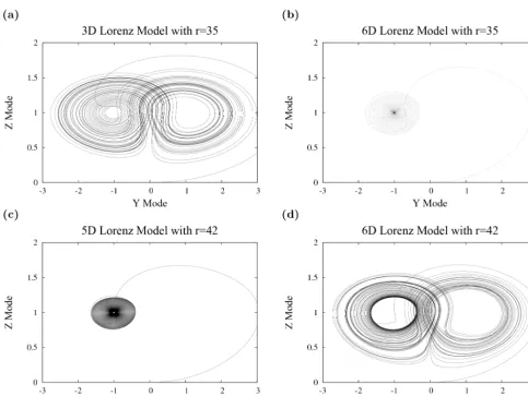
Next, we compare the normalized solutions of (Y,Z) in the 3DLM, 5DLM, and 6DLM with two different values of r. Normalization scales are defined by the critical points listed in Table 1. Figure 2a and b display the solutions from the 3DLM and 6DLM with r=35. Although the critical value (rc) for the onset of chaos isrc=24.74 in the 3DLM (Lorenz, 1963), a larger value is chosen for comparison with the 6DLM. The solution of the 3DLM never reaches a steady state but oscillates irregularly with time surrounding the non-trivial critical points. In contrast, as indicated by the con-verged trajectory that approaches a critical point that is close to(Y /Yc,Z/Zc)=(−1,1), the 6DLM yields a steady-state solution. Note that the normalization scales, Yc andZc, are the critical points of the 5DLM, because it is difficult to ob-tain the analytical solution of the critical points in the 6DLM and the former and latter share similarities as discussed later. The 6DLM continues to generate steady-state solutions un-tilris beyond 41.1 (as discussed in Fig. 4). With anrvalue of 42.0, the 6DLM leads to a chaotic solution with a “but-terfly” pattern inY–Zspace (Fig. 2d), while the 5DLM still produces a stable solution (Fig. 2c).
In the following, we discuss the time evolution of the solu-tions for the 5DLM and 6DLM to examine the impact of the
secondary modes on solution’s stability and to identify the major feedback associated with these modes. First, we ana-lyze the dZ/dτ (e.g., Eq. (10) for the 6DLM and Eq. (12) of Shen14 for the 5DLM) for the cases usingr=35 that have steady-state solutions. Figure 3 indicates that all of the terms with the exception ofX1Y, in the dZ/dτ of the 6DLM, yield comparable results to their counterparts in the 5DLM, indi-cating thatXY1 also plays an important role in stabilizing the solution of the 6DLM as compared to the 5DLM. While the negative feedback byXY1was verified by parameteriz-ing its impact as a nonlinear eddy dissipation term into the 3DLM in Shen14, further verification using the 6DLM is pro-vided in the following section. Due to a small value ofX1, theX1Y is small as compared to other terms. A small value ofX1could also be inferred from the steady-state solution to Eq. (11), givingX1=Y1/d2Y1as do=19/3. Addition-ally, the time evolution of theXYsuggests that a steady state in the 5DLM is reached earlier than it is in the 6DLM, con-sistent with the decay rate analysis in Sect. 3.1.
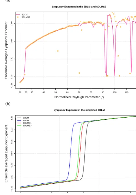
Figure 4 provides the analysis, used to determine the crit-ical value ofrfor the onset of chaos for both the 5DLM and 6DLM, of the eLEs as a function of the normalized Rayleigh parameterr. Both models produce similar distributions of the eLEs for 35≤r≤50, with the following features: (1) within the stable region (as eLEs<0), the magnitude of the eLEs is relatively smaller in the 6DLM; (2) the 6DLM requires a slightly smallerr (rc∼41.1) for the onset of chaos than the 5DLM (rc∼42.9); and (3) in fully chaotic regions (e.g., r >44), the eLEs of the 5DLM and 6DLM are in good agree-ment, with very small differences. The first two results are consistent with the stability analysis provided in Sect. 3.1, suggesting that inclusion of theM4mode in the 6DLM may reduce the dissipative impact associated with theM5mode. 3.3 Numerical results of the simplified 6DLMs
Figure 2. (Y,Z) plots in the 3DLM (a) and 6DLM (b) withr=35, and 5DLM (c) and 6DLM (d) withr=42. Lorenz strange attractors appear in (a) and (d). All of the solutions are normalized by the corresponding critical points, namely, Eq. (21) of Shen14 for the 3DLM and Eq. (19) of Shen14 for the 5DLM and 6DLM.
Figure 3. Forcing terms of dZ/dτwithr=35, which are from Eq. (12) for the 5DLM of Shen (2014a) (a) and Eq. (10) for the 6DLM (b),
respectively. The black and orange lines representXY andbZ, respectively, while the blue and red lines representXY1and 5X1Y,
Normalized Rayleigh Parameter (r)
Ensemb
le a
v
er
aged L
y
apuno
v Exponent
35 37 39 41 43 45 47 49
−0.25
0.00
0.25
0.50
0.75
1.00
1.25 5DLM6DLM
Lyapunov Exponent in the 5DLM and 6DLM
Figure 4. The largest ensemble-averaged Lyapunov exponents (eLEs) as a function of the forcing parameter r in different LMs. The eLEs with1r=0.1 for the 5DLM (black) and 6DLM (blue). The appearance of chaotic solutions is indicated by positive eLEs.
the window regions, indirectly indicating the importance of XY1in stabilizing the solutions in the 6DLM. With the ex-ception of the transition regions from eLEs<0 to eLEs>0 over a small range of r (i.e., r∼41–43), the eLEs of the 6DLMS1 and 6DLMS3 are close to those in the 6DLM and 5DLM. Thercof these two cases are determined to be 42.3 and 42.1, respectively, which are slightly larger (smaller) thanrc=41.1 (rc=42.9) for the 6DLM (5DLM), as shown in Fig. 5b. In addition, the magnitudes of the LEs in the sta-ble regions are determined to be relatively larger (smaller) than those in the 6DLM (5DLM). Since the 6DLMS1 ig-nores the nonlinear feedback terms associated with the X1 and since the 6DLMS3 neglects therX1term, the features of the 6DLMS1 and 6DLMS3, as compared to the 6DLM, also indicate that the impact of the M4 may slightly destabilize solutions.
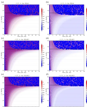
The eLEs represent the averaged behavior of the model’s solutions over a very large timescale, soN=10 000 000 and T =N4t=1000 (e.g., theT in Eq. (23) of Shen14 should approach infinity) are used. Since some of the terms in the simplified LMs (e.g., 6DLMS1-3) are ignored, it is impor-tant to check the time evolution of the solutions on a finite timescale in order to understand whether and how the so-lutions approach a stable critical point, or oscillate rapidly between (unstable) non-trivial critical points. To this end, we examine ther time diagram of the normalized solutions in Fig. 6, which displays the primary mode, −Y /Yc, and secondary mode, −Y1/Y1c, from the 6DLM, 6DLMS1, and 6DLMS3. Here,YcandY1care the analytical solutions of the critical points from the 5DLM. Using this approach, the de-viation of the normalized solutions from 1 (i.e.,−Y /Yc−1) indicates the impact of the M4mode that is missing in the 5DLM. In Fig. 6, the sharp gradient of the solutions with dense contour lines near the constant value of r=43 (in black) roughly indicates the critical value ofrfor the onset
(a)
Normalized Rayleigh Parameter (r)
Ensemb
le a
v
er
aged L
y
apuno
v Exponent
20 25 30 40 50 60 70 80 90 100 110 120
−0.25
0.00
0.50
1.00
1.50
3DLM 6DLMS2
Lyapunov Exponent in the 3DLM and 6DLMS2
(b)
Normalized Rayleigh Parameter (r)
Ensemb
le a
v
er
aged L
y
apuno
v Exponent
35 37 39 41 43 45 47 49
−0.25
0.00
0.25
0.50
0.75
1.00
1.25 5DLM6DLM 6DLMS1 6DLMS3
Lyapunov Exponent in the simplified 6DLM
Figure 5. Same as Fig. 4 except for (a) the 3DLM (in pink) and the 6DLMS2 (in orange), and (b) the 6DLMS1 (in red) and 6DLMS3 (in green).
of chaos, consistent with the analysis of the eLEs in Fig. 5 (see Table 1). In stable regions, the primary mode,−Y /Yc, evolves with time and comes within 1±0.01 in each of the three cases (Fig. 6a, c, e). For the 6DLMS1 that only in-cludes one nonlinear feedback term (XY1), the values of the secondary mode,−Y1/Y1c, in stable regions are also within 1±0.01 (Fig. 6d). By comparison, the normalized solutions (−Y1/Y1c) for the 6DLM and 6DLMS3 are within 1 and 0.9 in the steady state, suggesting a deviation within 10 % from the corresponding critical point of the 5DLM. If we view the stable solutions of the 5DLM as the results of the control run, the 6DLM provides approximate steady-state solutions that have derivations of only around 1 % inY and approximately 10 % in Y1. The above results indicate that the nonlinear terms associated with theX1(i.e.,M4mode) may produce larger relative deviations in the secondary modeY1(a high-wavenumber mode) than in the primary modeY(a low wave-number mode).
im-Figure 6. Ther-time diagram of numerical solutions from the 6DLM (a, b), 6DLMS1 (c, d), and 6DLMS3 (e, f).rranges from 25 to 50 with1r=0.5. (a, c, e) show−Y /Yc, and (b, d, f) show−Y1/Y1c.YcandY1care the critical points of the 5DLM as defined in Eq. (19) of
Shen14. The black line indicates a constant value ofr=43.
proved by the negative nonlinear feedback through the term (−XY1), enabled by the secondary temperature modes (Y1 and Z1) in the 5DLM. The result motivated an examina-tion of whether or not a higher-dimensional model is more stable or less chaotic (i.e., a larger critical value of r) than a lower-dimensional model. In this study, the comparison of the 5DLM and 6DLM indicates that the additional mode (M4) in the 6DLM does not help increase but slightly de-creases the critical value ofrfor the onset of chaos. In other words, the inclusion of M4 provides positive feedback that destabilizes the solutions through the heating term (e.g.,rX1
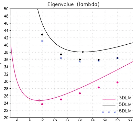
Figure 7. Thercof the 6DLM as a function ofσ. Therc, shown by
blue multiplication signs (X), is determined by the eLEs of the non-linear 6DLM. The pink and black lines indicate a constant contour of Re(λ)=0 for the linear 3DLM and 5DLM, respectively, indicat-ing the correspondindicat-ingrc, based on a linear stability analysis. Solid
circles with the same color scheme indicate arc, determined by the
eLE analysis with1r=0.1 in the corresponding nonlinear LM.
3.4 Dependence of stability onσ
Previous sections discussed the stability problem only by varying the heating parameter,r. Here, we examine the de-pendence of solution stability on the parameter σ, and ad-dress the question of whether or not the 6DLM still requires a smaller (larger) rc for the onset of chaos than the 5DLM (3DLM) when different values ofσ are used. To efficiently achieve the goal, we conduct the eLE analysis for the 6DLM using selected values ofσ, and compare it with that from the 5DLM. The dependence of the 5DLM’s stability on σ was previously examined by Shen14 by performing both linear stability and eLE analyses.
For comparisons, the results obtained from the stability analysis of the 5DLM and 3DLM in Shen14 are briefly sum-marized as follows: in Fig. 7, pink and black lines indicate the contour lines of the Re(λ)=0 in the (σ, r) space for the linearized 3DLM and 5DLM, respectively. Sinceλis the largest eigenvalue, each line describes the critical valuerclas a function ofσ, where the superscript “l” ofrclindicates the local (or linear) analysis. Following each of the contour lines in the direction of increasingσ, its right (or left) hand side contains areas with negative (or positive) values of Re(λ), suggesting stable (or unstable) solutions. Therefore, unsta-ble solutions (Re(λ) >0) appear asrcl< r. Solid circles with the same color scheme indicate therc determined using the eLE analysis with selected values ofσ:σ=10, 13, 16, 19,
22 and 25. Given aσ, rc is, in general, smaller thanrcl in both the 3DLM and 5DLM, as previously documented (see Shen14 for additional details).
The rc of the 6DLM, with the eLE analysis, is shown in Fig. 7 with blue multiplication signs. For all of the se-lected cases, the critical valuercin the 6DLM is larger than that in the 3DLM, suggesting that over the range between σ=10∼25, the 6DLM requires a largerr for the onset of chaos than the 3DLM. By comparison, in each of the selected cases withσ=10, 13, 16, and 19, the critical value (rc) in the 6DLM is (slightly) smaller than the one in the 5DLM. As a result, the 6DLM is less stable than the 5DLM as 10≤r <22. However, for the case withσ=22 (orσ=25), thercof the 6DLM is comparable (or slightly larger), as com-pared to that of the 5DLM. The results may indicate a differ-ent role for the M4 mode between σ <22 and σ >22, or suggest the importance of increasing the ensemble members and/or increasing the coverage of the initial conditions for the calculations of the eLEs, all of which are subject to fu-ture study.
4 Concluding remarks
Five- and six-dimensional Lorenz models (5DLM and 6DLM) were derived here and in Shen14 to examine the im-pact of additional modes on solution’s stability. The 5DLM includes two new Fourier modes (i.e., the secondary temper-ature modesM5andM6) that introduce the additional non-linear and dissipative terms. The 6DLM is a super set of the 5DLM, and contains one more Fourier mode (i.e., the sec-ondary streamfunction modeM4) that introduces additional nonlinear terms and adds a heating term. The individual and collective impacts of these terms on solution stability were investigated. The 5DLM and 6DLM have comparable criti-cal Rayleigh parameters for the onset of the chaos, and the parameters are larger than that of the 3DLM. Based on the calculations of the ensemble-averaged Lyapunov exponents (eLEs), the critical value rc for the 6DLM (5DLM) with σ=10 is approximately 41.1 (42.9). Therefore, while the so-lution of the 3DLM becomes chaotic whenrranges from 25 to 40, the 6DLM (5DLM) still produces stable steady-state solutions, suggesting that predictability can be improved by the increased degree of nonlinearity.
M5mode, and, in turn, provides effective “positive” feedback through the nonlinear feedback loop; (3) as a result of much smaller values in theX1, the induced destabilization (by the additional heating term) is much smaller than the induced stabilization (by the negative nonlinear feedback term). Ad-ditionally, two nonlinear feedback terms associated withM4 nearly cancel one another (e.g., Eqs. 32 and 33). Therefore, therc of the 6DLM is only slightly smaller than that of the 5DLM. The 5DLM and 6DLM collectively illustrate the dif-ferent roles of various high-wavenumber modes in stablizing or destabilizing a system’s solutions. Additional analyses of mathematical derivations and numerical results are summa-rized below.
As compared to the 3-D and 5-D LMs in the dissipation-less limit, the 6-D non-dissipative LM also poses two en-ergy conservation relations. One states the conservation of the total domain-averaged kinetic energy (KE) and available potential energy (APE), enabling the transfer between KE and APE. The result is consistent with the result in the 3-D and 5-D non-dissipative LMs. In contrast, the additional con-servation law only provides the concon-servation of the domain-averaged kinetic energy associated with the primary stream-function mode (KEp) and the total domain-averaged potential energy (PE), instead of the total KE and PE, as compared to the 3DLM and 5DLM. The two conservations do pose con-straints on all six modes of the 6DLM. However, the poten-tial issues (e.g., whether inconsistent forcing may exist) are beyond the scope of the present study.
The competing impact of the nonlinearities and the dissi-pation and heating terms can be illustrated using Eq. (10) of the 6DLM, as follows:
dZ
dτ =XY−XY1−X1Y−bZ.
The first nonlinear term (XY) and the linear term (bZ) can act as a forcing and dissipative term, respectively, in the 3-D, 5-3-D, and 6-D LMs. The second and third nonlinear terms (XY1andX1Y) are introduced as additional dissipative terms by the new modes.X1Y is much smaller than the other terms, andXY1can help reach a balance withXY andbZto stabi-lize the solution. The negative nonlinear feedback by XY1 was first illustrated by Shen14 for the 5DLM. However, the feedback by XY1in the 6DLM may be (slightly) different from that in the 5DLM. Specifically, whileXY1of the 5DLM includes the feedback associated with additional nonlinear and dissipative terms, XY1of the 6DLM includes the feed-back from the additional nonlinear and heating terms such as rX1.
The above results provide different impacts associated with various secondary modes, consistent with Lorenz’s statement in 1972, as follows: “If the flap of a butterfly’s wings can be instrumental in generating a tornado, it can equally well be instrumental in preventing a tornado.” The quote suggests the appearance of both positive and nega-tive feedbacks (i.e., stabilization and destabilization) in
as-sociation with various “small-scale” processes. Since mode truncation is unavoidable in finite-resolution models, the an-swer to the question of whether or not the feedback by new modes is positive or negative should be made in the proper context. The approach outlined here may help us understand why some generalized LMs have a larger rc while others have a smaller rc as compared to the 3DLM. For exam-ple, among the five different generalized LMs in Tables 1 and 2 of Roy and Musielak (2007c), the two LMs that in-cludeM5 andM6have arc of∼40–42, comparable to the rc in the 5DLM (6DLM) outlined here. The 22(1,3) and 22(0,4)modes in Roy and Musielak (2007c) are the same as theM5andM6modes in this study. In addition, the 14-D LM, with a comparablerc (rc∼43.48) described by Curry (1978), also includes these two modes22(1,3)and22(0,4), and does not have a vertical wavenumber higher than that of22(0,4). In contrast, the 5-D LM of Roy and Musielak (2007b), which has a smallerrc(rc∼22.5), does include an additional heating term, although the two additional modes are different from the secondary modes of the 5DLM and 6DLM in this study. Although preliminary analyses seem encouraging, however, detailed comparisons with other gen-eralized LMs (e.g., Howard and Krishnamurti, 1986; Her-miz et al., 1995; Thiffeault and Horton, 1996) are still re-quired. In addition, the further extension of the nonlinear feedback loop is being studied withM7−M9 modes, here M7=
√
2 sin(lx)sin(5mz), M8= √
2 cos(lx)sin(5mz), and M9=sin(6mz). Preliminary results indicates that a larger rc is required for the onset of chaos (e.g.,rc=116.9 for the 7DLM withM8andM9modes). Using a 3-D non-dissipative Lorenz model, which is shown to be a conservative system, we discussed the collective and competing impact of the non-linear feedback loop and heating term on the energy cycle with four different regimes (e.g., Shen, 2014b). We will fur-ther analyze the energy cycle in the higher-order dissipative or non-dissipative Lorenz models using the same approach and compare the results with those using a different approach (e.g., Pelino et al., 2014).
Appendix A: Fractal dimension of the 6DLM
Various methods are available for calculating fractal dimen-sions. There are several mathematical definitions of differ-ent types of fractal dimension (Grassberger and Procaccia, 1983; Nese et al., 1987; Ruelle, 1989; Zeng et al., 1992). In this study, we only discuss the method for calculating the so-called Kaplan–Yorke dimension (Dky), which requires the calculation of Lyapunov exponents (LEs) and thus can be used for the verification of LE calculation. The Kaplan– Yorke dimension is defined as follows (Kaplan and Yorke, 1979; Nese et al., 1987):
Dky=K+ PK
i=1LEi |LEK+1|
, (A1)
where LEi is the ith Lyapunov exponent, and K(≤n) is
the largest integer for which PK
i=1LEi≥0. Dky=0 as LE1<0 and Dky=n as Pni=1LEi>0. In this study, “n”
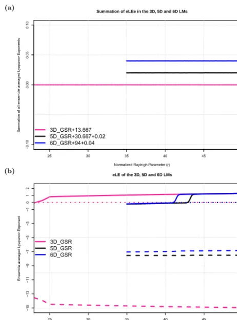
ensemble-averaged Lyapunov exponents (eLEs), which are produced using the GSR method (e.g., Shen14), are used to estimate the corresponding Dky. The summation of all eLEs is provided in Fig. A1a, where −13.667, −30.667, and−94 are the values for the 3DLM, 5DLM and 6DLM, respectively, and are consistent with the stability analysis. For example, in the 6DLM, the summation of all eLEs should be equal to−(σ+1+b+doσ+do+4b). The three leading eLEs for the 3DLM, 5DLM and 6DLM are pro-vided in Fig. A1b. The corresponding fractal dimension obtained using the eLEs is provided in Fig. A2. For r=
28, the leading eLEs of the 3DLM are (0.892743×10+0,
−0.701148×10⁻³, −0.145587×10+2), which results in Dky=2.06127208. The value is very close to the value of 2.063 documented in Nese et al. (1987, p. 1957) and the value of 2.062 reported by Sprott (http://sprott.physics.wisc.edu/ chaos/lorenzle.htm). Here, the reader should note that the second eLE is very small but not exactly equal to zero, in-dicating the impact of the 10 000 different initial conditions and/or the “finite” integration time (T =1000) in this study.
(a)
Normalized Rayleigh Parameter (r)
Summation of all ensemb
le a
ver
aged L
yapuno
v Exponents
25 30 35 40 45 50
−0.10
0.00
0.05
0.10
3D_GSR+13.667 5D_GSR+30.667+0.02 6D_GSR+94+0.04
Summation of eLEe in the 3D, 5D and 6D LMs
(b)
Normalized Rayleigh Parameter (r)
Ensemb
le a
ver
aged L
yapuno
v Exponent
25 30 35 40 45 50
−15
−13
−11
−9
−7
−5
−3
−1
0
1
2
3D_GSR 5D_GSR 6D_GSR
eLE of the 3D, 5D and 6D LMs
Figure A1. The summation of all ensemble-averaged Lyapunov exponents (eLEs) in the LMs (a) and three leading ensemble-averaged Lyapunov exponents (eLEs) as a function of the normal-ized Rayleigh number (r) (b). The pink, black, and blue lines indi-cate the eLEs for the 3-D, 5-D and 6-D LMs, respectively. The solid, dotted, and dashed lines display the first, second and third eLEs, re-spectively. In (a), the pink, black, and blue lines are shifted with a constant value of 13.667, 30.667+0.02 and 94.0+0.04, respec-tively. To save computational resources, the eLEs of the 5-D and 6-D LMs are calculated over a shorter range of values forr (i.e., 35< r <50).
Normalized Rayleigh Parameter (r)
Fr
actal dim
25 30 35 40 45 50
2.00
2.05
2.10
2.15
2.20 3D_GSR5D_GSR 6D_GSR
Fractal dimension of the 3D, 5D and 6D LMs
The Supplement related to this article is available online at doi:10.5194/npg-22-749-2015-supplement.
Acknowledgements. We thank V. Lucarini, one anonymous re-viewer, S. Vannitsem (Editor), Y.-L. Lin, R. Anthes, X. Zeng, and R. Pielke Sr. for valuable comments and encouragement. We are grateful for support from the NASA Advanced Information System Technology (AIST) program of the Earth Science Technology Office (ESTO) and from the NASA Computational Modeling Algorithms and Cyberinfrastructure (CMAC) program. Resources supporting this work were provided by the NASA High-End Computing (HEC) program through the NASA Advanced Super-computing division at Ames Research Center.
Edited by: S. Vannitsem
Reviewed by: V. Lucarini and one anonymous referee
References
Anthes, R.: Turning the tables on chaos: is the atmosphere
more predictable than we assume?, UCAR Magazine,
available at: https://www2.ucar.edu/atmosnews/opinion/
turning-tables-chaos-atmosphere-more-predictable-we-assume-0, last access: 14 December 2015, 2011.
Benettin, G., Galgani, L., Giorgilli, A., and Strelcyn, J. M.: Lya-punov Characteristic Exponents fro Smooth Dynamical Systems and for Hamiltonian Systems; A method for computing all of them. Part 1: Theory, Meccanica, 15, 9–20, 1980.
Blender, R. and Lucarini, V.: Nambu representation of an extended Lorenz model with viscous heating, Physica D, 243, 86–91, 2013.
Chen, Z.-M. and Price, W. G.: On the relation between Raleigh-Benard convection and Lorenz system, Chaos Soliton. Fract., 28, 571–578, 2006.
Christiansen, F. and Rugh, H.: Computing Lyapunov spectra with continuous Gram–Schmid orthonormalization, Nonlinearity, 10, 1063–1072, 1997.
Curry, J. H.: Generalized Lorenz systems, Commun. Math. Phys., 60, 193–204, 1978.
Curry, J. H., Herring, J. R., Loncaric, J., and Orszag, S. A.: Order and disorder in two- and three-dimensional Benard convection, J. Fluid. Mech., 147, 1–38, 1984.
Ding, R. O. and Li, J. P.: Nonlinear finite-time Lyapunov exponent and predictability, Phys. Lett., 354, 396–400, 2007.
Eckhardt, B. and Yao, D.: Local Lyapunov exponents in chaotic sys-tems, Physica D, 65, 100–108, 1993.
Franceschini, V. and Tebaldi, C.: Truncations to 12, 14 and 18 Modes of the Navier-Stokes Equations on a Two-Dimensional Torus, Meccanica, 20, 207–230, 1985.
Franceschini, V., Giberti, C., and Nicolini, M.: Common Period Be-havior in Larger and Larger Truncations of the Navier Stokes Equations, J. Stat. Phys., 50, 879–896, 1988.
Froyland, J. and Alfsen, K. H.: Lyapunov-exponent spectra for the Lorenz model, Phys. Rev. A, 29, 2928–2931, 1984.
Gleick, J.: Chaos: Making a New Science, Penguin, New York, 360 pp., 1987.
Grassberger, P. and Procaccia, I.: Characterization of strange attrac-tors, Phys. Rev. Lett., 5, 346–349, 1983.
Hermiz, K. B., Guzdar, P. N., and Finn, J. M.: Improved low-order model for shear flow driven by Rayleigh–Benard convection, Phys. Rev. E, 51, 325–331, 1995.
Howard, L. N. and Krishnamurti, R. K.: Large-scale flow in tur-bulent convection: a mathematical model, J. Fluid Mech., 170, 385–410, 1986.
IPCC: Climate Change 2007: The Physical Science Basis, in: Con-tribution of Working Group I to the Fourth Assessment Report of the Intergovernmental Panel on Climate Change, edited by: Solomon, S., Qin, D., Manning, M., Chen, Z., Marquis, M., Av-eryt, K. B., Tignor, M., and Miller, H. L., Cambridge Univer-sity Press, Cambridge, UK and New York, NY, USA, 996 pp., available at: http://www.ipcc.ch/pdf/assessment-report/ar4/wg1/ ar4-wg1-faqs.pdf, last access: 14 December 2015, 2007. Kaplan, J. L. and Yorke, J. A.: Chaotic behavior of
multidimen-sional difference equations, in: Functional Differential Equa-tions and the ApproximaEqua-tions of Fixed Points, edited by: Peit-gen, H. O. and Walther, H. O., Springer-Verlag, New York, Lect. Notes Math., 730, 228–237, 1979.
Kazantsev, E.: Local Lyapunov exponents of the quasi-geostrophic ocean dynamics, Appl. Math. Comput., 104, 217–257, 1999. Kennamer, K. S.: Studies of the onset of chaos in the Lorenz and
generalized Lorenz systems, MS thesis, The University of Al-abama, Huntsville, USA, 1995.
Li, J. and Ding, R.: Temporal-Spatial Distribution of atmospheric predictability limit by local dynamical analogs, Mon. Weather Rev., 139, 3265–3283, 2011.
Lorenz, E.: Deterministic nonperiodic flow, J. Atmos. Sci., 20, 130– 141, 1963.
Lorenz, E.: Predictability: does the flap of a butterfly’s wings in Brazil set off a tornado in Texas?, in: American Association for the Advancement of Science, 139th Meeting, 29 Decem-ber 1972, Boston, Mass., AAAS Section on Environmental Sci-ences, New Approaches to Global Weather, GARP, available at: http://eaps4.mit.edu/research/Lorenz/Butterfly_1972.pdf, last access: 14 December 2015, 1972.
Lucarini, V. and Fraedrich, K.: Symmetry breaking, mix-ing, instability, and low-frequency variability in a
min-imal Lorenz-like system, Phys. Rev. E, 80, 026313,
doi:10.1103/PhysRevE.80.026313, 2009.
Musielak, Z. E., Musielak, D. E., and Kennamer, K. S.: The onset of chaos in nonlinear dynamical systems determined with a new fractal technique, Fractals, 13, 19–31, 2005.
Nese, J. M.: Quantifying local predictability in phase space, Phys-ica, 35, 237–250, 1989.
Nese, J. M., Dutton, J. A., and Wells, R.: Calculated attractor dimen-sions for low-order spectral models, J. Atmos. Sci., 44, 1950– 1972, 1987.
Pelino, V., Maimone, F., and Pasini, A.: Energy cycle for the Lorenz attractor, Chaos Soliton. Fract., 64, 67–77, 2014.
Pielke, R.: The Real Butterfly Effect, available at:
http://pielkeclimatesci.wordpress.com/2008/04/29/
the-real-butterfly-effect/, last access: 14 December 2015, 2008.
Roy, D. and Musielak, Z. E.: Generalized Lorenz models and their routes to chaos, II. Energy-conserving horizontal mode trunca-tions, Chaos Soliton. Fract., 31, 747–756, 2007b.
Roy, D. and Musielak, Z. E.: Generalized Lorenz models and their routes to chaos, III. Energy-conserving horizontal and vertical mode truncations, Chaos Soliton. Fract., 33, 1064–1070, 2007c. Ruelle, D.: Chaotic Evolution and Strange Attractors, in: Lezioni Lincee, Cambridge University Press, Cambridge, doi:10.1017/CBO9780511608773, 1989.
Saltzman, B.: Finite amplitude free convection as an initial value problem, J. Atmos. Sci., 19, 329–341, 1962.
Shen, B.-W.: Nonlinear feedback in a five-dimensional Lorenz model, J. Atmos. Sci., 71, 1701–1723, doi:10.1175/JAS-D-13-0223.1, 2014a.
Shen, B.-W.: On the nonlinear feedback loop and energy cycle of the non-dissipative Lorenz model, Nonlin. Processes Geophys. Discuss., 1, 519–541, doi:10.5194/npgd-1-519-2014, 2014b. Shen, B.-W.: Parameterization of Negative Nonlinear Feedback
using a Five-dimensional Lorenz Model, Fractal Geometry and Nonlinear Analysis in Medicine and Biology, 1, 33–41, doi:10.15761/FGNAMB.1000109, 2015.
Shen, B.-W., Atlas, R., Reale, O., Lin, S.-J., Chern, J.-D., Chang, J., Henze, C., and Li, J.-L.: Hurricane forecasts with a global mesoscale-resolving model: Preliminary results with Hurricane Katrina (2005), Geophys. Res. Lett., 33, L13813, doi:10.1029/2006GL026143, 2006.
Shen, B.-W., Tao, W.-K., Lin, Y.-L., and Laing, A.: Genesis of twin tropical cyclones as revealed by a global mesoscale model: the role of mixed Rossby gravity waves, J. Geophys. Res., 117, D13114, doi:10.1029/2012JD017450, 2012.
Shen, B. W., DeMaria, M., Li, J.-L. F., and Cheung, S.: Genesis of hurricane Sandy (2012) simulated with a global mesoscale model, Geophys. Res. Lett., 40, 4944–4950, doi:10.1002/grl.50934, 2013.
Sprott, J. C.: Numerical Calculation of Largest Lyapunov Expo-nent, available at: http://sprott.physics.wisc.edu/chaos/lyapexp. htm, last access: 14 December 2015, 1997.
Sprott, J. C.: Chaos and Time-Series Analysis, Oxford University Press, 528 pp., 2003.
Thiffeault, J.-L. and Horton, W.: Energy-conserving truncations for convection with shear flow, Phys. Fluids, 8, 1715–1719, 1996. Treve, Y. M. and Manley, O. P.: Energy conserving Galerkin
ap-proximations for 2-D hydrodynamic and MHD Benard Convec-tion, Physica, 4, 319–342, 1982.
Wolf, A., Swift, J. B., Swinney, H. L., and Vastano, J. A.: Determin-ing Lyapunov exponents from a time series, Physica, 16, 285– 317, 1985.
Zeng, X., Eykholt, R., and Pielke, R. A.: Estimating the Lyapunov-exponent spectrum from short time series of low precision, Phys. Rev. Lett., 66, 3229–3232, 1991.