https://doi.org/10.5194/esd-8-707-2017
© Author(s) 2017. This work is distributed under the Creative Commons Attribution 3.0 License.
On determining the point of no return in climate change
Brenda C. van Zalinge, Qing Yi Feng, Matthias Aengenheyster, and Henk A. Dijkstra
Institute for Marine and Atmospheric Research Utrecht, Department of Physics, Utrecht University, Utrecht, the Netherlands
Correspondence to:Qing Yi Feng ([email protected])
Received: 13 September 2016 – Discussion started: 16 September 2016 Revised: 21 June 2017 – Accepted: 3 July 2017 – Published: 9 August 2017
Abstract. Earth’s global mean surface temperature has increased by about 1.0◦C over the period 1880–2015. One of the main causes is thought to be the increase in atmospheric greenhouse gases. If greenhouse gas emis-sions are not substantially decreased, several studies indicate that there will be a dangerous anthropogenic in-terference with climate by the end of this century. However, there is no good quantitative measure to determine when it is “too late” to start reducing greenhouse gas emissions in order to avoid such dangerous interference. In this study, we develop a method for determining a so-called “point of no return” for several greenhouse gas emission scenarios. The method is based on a combination of aspects of stochastic viability theory and linear response theory; the latter is used to estimate the probability density function of the global mean surface tem-perature. The innovative element in this approach is the applicability to high-dimensional climate models as demonstrated by the results obtained with the PlaSim model.
1 Introduction
In the year 2100, which is as far (or as close) in the future as 1932 is in the past, mankind will be living on an Earth with a different climate than today. At that time, we will know the 2100 global mean surface temperature (GMST) value and its increase,1T, above the pre-industrial GMST value. From the then available GMST records, it will also be known whether this change in GMST has been gradual or whether it was rather “bumpy”. If the observational effort continues as of today, there will also be an adequate observational record to determine whether the probability of extreme events (e.g. flooding, heat waves) has increased.
The outcomes of these future observations to be made by future generations will strongly depend on the socio-economic and technological developments and political deci-sions made now and over the next decades. Fortunately, there is a set of tools available to inform decision makers: Earth system models. These models come in different flavours, from global climate models (GCMs) providing details on the development of the ocean–atmosphere–ice–land system to integrated assessment models (IAMs), which also aim to describe the development of the broader socio-economic
sys-tem. During the preparation for the fifth assessment report (AR5) of the Intergovernmental Panel on Climate Change (IPCC), GCM studies have focussed on the climate system response to GHG changes as derived by IAMs from dif-ferent socio-economic scenarios; the data from these sim-ulations are gathered in the so-called CMIP5 archive (http: //cmip-pcmdi.llnl.gov/cmip5/).
Depending on the representation of fast climate feedbacks in GCMs that determine their climate sensitivity, the CMIP5 models project a GMST increase1T of 2.5–4.5◦C over the period 2000–2100 (Pachauri et al., 2014). This does not mean that the actual measured value of1T in 2100 will be in this interval. For example, the GMST may be well outside this range because of current model errors which misrepresent the strength of a specific feedback. As a consequence, a tran-sition might have occurred in the real climate system which did not occur in any of the CMIP5 model simulations. An-other possibility is that the GHG development was eventually far outside of the scenarios considered in CMIP5.
and extreme events will have increased in frequency and magnitude (Smith and Schneider, 2009). These effects are very inhomogeneously distributed over the Earth and lead to enormous socio-economic consequences. If this is the case in 2100, then there is a point in time at which we must have crossed the conditions for DAI. This time, marking the boundary of a “safe” and “unsafe” climate state, obviously depends on the metrics used to quantify the state of the com-plex climate system.
In very simplified views, this boundary is interpreted as a threshold CO2concentration (Hansen et al., 2008) or GMST. The latter, in particular the 1Tc=2◦C threshold, has
be-come an easy to communicate (and maybe therefore leading) idea to set mitigation targets for greenhouse gas reduction. Emission scenarios have been calculated (Rogelj et al., 2011) such that1T will remain below1Tc. Although thresholds
for GMST have been criticized for being very inadequate re-garding impacts (Victor and Kennel, 2014), such a threshold forms the basis for policymaking as set forward in the Paris 2015 (COP21) agreement.
Supposing that measures are being taken to keep 1T < 1Tc, does this mean that we are “safe”? The answer is a
sim-ple no, as DAI may still have occurred regionally, such as the disappearance of island chains due to sea level rise (Victor and Kennel, 2014). Hence, attempts have been made to de-fine what “safe” means in a more general way, such as the tol-erable windows approach (TWA; Petschel-Held et al., 1999) and viability theory (VT; Aubin, 2009). These approaches also deal with general control strategies to steer a system to-wards “safety” when needed.
On a more abstract level, both TWA and VT start by defin-ing a desirable (or “safe”) subspaceV of a state vectorxin a general state space X. This subspace is characterized by constraints, such as thresholds for properties of x. For ex-ample, whenxis a high-dimensional state vector of a GCM, such a threshold could be 1T < 1Tc for GMST. When the
time development (or trajectory) of x is such that it moves outside the subspaceV, a control is sought to steer the tra-jectory back intoV. Note that this is an abstract formulation of the mitigation problem when the amplitude of the green-house gas emission is taken as a control. Recently, (Heitzig et al., 2016) have added more detail to regions in the space Xwhich differ in their “safety” properties and the amount of flexibility in the control to steer to “safety”.
Given a certain desirable subspace of the climate system state vector (e.g. to avoid DIA) and a suite of control options (e.g. CO2emission reduction), it is important to know when it is too late to steer the system to “safe” conditions, for ex-ample in the year 2100. In other words, when is the point of no return (PNR)? The TWA and VT approaches and the the-ory in (Heitzig et al., 2016) suffer from the “curse of dimen-sionality” and cannot be used within CMIP5 climate models. For example, the optimization problems in VT and TWA lead to dynamic programming schemes which have up to now only been solved for model systems with low-dimensional
state vectors. The approach in (Heitzig et al., 2016) requires the computation of regional boundaries in state space, which also becomes tedious in more than two dimensions. Hence, with these approaches it will be impossible to determine a PNR using reasonably detailed models of the climate system. In this paper, we present an approach similar to TWA and VT, but one which can be applied to high-dimensional mod-els of the climate system. The key to the approach is the estimation of the probability density function of the prop-erties of the state vectorx which determine the “safe” sub-spaceV. The PNR problem is coupled to limitations in the control options (e.g. of emissions) and can be defined pre-cisely using these options and stochastic viability theory. The methodology is presented in Sect. 2; to illustrate the con-cepts, we apply the approach in Sect. 3 to an idealized en-ergy balance model with and without tipping behaviour. In Sect. 4, the application to a high-dimensional climate model is presented using data from the Planet Simulator (PlaSim; Fraedrich et al., 2005). A summary and discussion in Sect. 5 concludes the paper.
2 Methodology
Here we briefly describe the concepts we need from stochas-tic viability theory and then define the PNR problem, specif-ically in the climate change context.
2.1 Viable states
Viability theory studies the control of the evolution of dy-namical systems to stay within certain constraints on the system state vector (Aubin, 2009). Here we consider finite dimensional deterministic systems with state vectorx∈Rd and vector fieldf :Rd→Rdgiven by
dx
dt =f(x, t). (1)
In the general formulation of viability theory, a time-dependent input is also considered on the right-hand side of Eq. (1), which can be used to control the path of the trajectory x(t) in state space.
Stochastic extensions of viability theory consider finite dy-namical systems defined by stochastic differential equations:
dXt=f(Xt, t)dt+g(Xt, t)dWt, (2)
where Xt∈Rd is a multidimensional stochastic process,
Wt ∈Rn is a vector ofn-independent standard Wiener
pro-cesses, and the matrixg∈Rd×ndescribes the dependence of the noise on the state vector. The normalized probability den-sity function (PDF)p(x, t) can be formally determined from the Fokker–Planck equation associated with Eq. (2).
A stochastic viability kernelVβ consists of initial
condi-tionsX0for which the system has, for 0≤t≤t∗, a probabil-ity larger than a valueβto stay in the viable regionV (Doyen and De Lara, 2010). For example, in a one-dimensional ver-sion of Eq. (2) with state vectorXt ∈R and a viable region V given byx≤x∗, a stateXt is called viable with tolerance
probabilityβTif
x∗ Z
−∞
p(x, t)dx≥βT; (3)
otherwise,Xt is called non-viable.
2.2 Linear response theory
In relatively idealized low-dimensional models (such as the energy balance model in Sect. 3), the probability density functions can be easily computed by solving for the Fokker– Planck equation (see Sect. 3.2). However, in order to find the temporal evolution of the PDF of the global mean surface temperature (GMST) under any CO2-equivalent forcing in high-dimensional climate models, such as PlaSim in Sect. 4, we will use linear response theory (LRT). With this theory, the effect of any small forcing perturbation on the system state can be calculated by running the climate model for only one forcing scenario (Ragone et al., 2016).
In LRT, the expectation value of an observable 8, when forcing the system with a time-dependent functionf(t), can be calculated by computing the convolution of a Green’s functionGh8iand the forcingf(t) according to
h8if(t)= +∞ Z
−∞
Gh8i(τ)f(t−τ)dτ. (4)
To construct this Green’s function, the property that the con-volution in the time domain is the same as pointwise multi-plication in the frequency domain is used. The Fourier trans-form of Eq. (4) is given by
he8if(ω)=χh8i(ω)fe(ω), (5)
withχh8i(ω),he8if(ω), andfe(ω) as the Fourier transforms of Gh8i(t),h8if(t), andf(t), respectively. Therefore, once
the time evolution of the expectation value of an observable under a certain forcing is known, the Green’s function of this observable can be constructed with Eq. (5), and consequently the linear response of the observable to any forcing can be calculated.
2.3 The point of no return problem
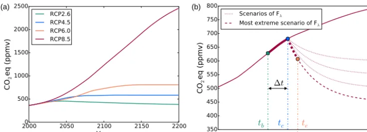
In the climate change context, scenarios of GHG increase and the associated radiative forcing have been formulated as representative concentration pathways (RCPs). In (Pachauri et al., 2014), there are four RCP scenarios (Fig. 1a) ranging from an increase in radiative forcing of 2.6 Wm−2(RCP2.6) in 2100 (with respect to 2000) to a forcing increase of 8.5 Wm−2(RCP8.5).
To define the PNR for each of these RCPs, a collection of mitigation scenarios on greenhouse gas emissions has to be considered. These mitigation scenarios will lead to changes in GHG concentrations described by functionsFλ(t), where λis a parameter. For instance, the collectionFλcould result
from mitigation measures that lead to an exponential decay to different stabilization levels (measured in CO2equivalent, or CO2eq.) within a certain time interval. An example of such a collectionFλis shown by the dashed and dotted red lines
in Fig. 1b. The most extreme member ofFλis defined as the
mitigation scenario (represented by a certain value of param-eterλ) which has the steepest initial decrease at a certain time t(dashed curve in Fig. 1b).
Along the curve of a certain RCP scenario, there will be a point in time at which action will be taken to reduce emis-sions of GHG; this is indicated by a time of actiontb.
Con-sider, for example (Fig. 1b), thattbis chosen as the first year
in which the state vectorXt is no longer viable. A
reduc-tion in emissions is, however, not immediately followed by a decrease in CO2eq. due to the long residence time of at-mospheric CO2. In addition, there is a delay to take action in emission reduction due to technological, social, economic, and institutional challenges. Hence, emission reduction will only start 1t1 years after tb. The CO2eq. will, even after emissions have been reduced, also still increase over a time 1t2. The time at which the CO2eq. starts to reduce accord-ing toFλis indicated bytc=tb+1t, where1t=1t1+1t2.
Eventually, Xt may become viable again and this point in
time is indicated byte(Fig. 1b).
For a given RCP scenario, tolerance probabilityβT, viable regionV, and collectionFλ, we define the PNR (πt) as the
first yeartc in which, even when at that moment the most
extreme CO2-equivalent reduction scenarioFλapplies,
a. either Xt will be non-viable for more than τT years,
whereτTis a set tolerance time, or
b. Xt will be non-viable in the year 2100.
t
350400 450 500 550 600 650 700 750 800
CO
2eq
(p
pm
v)
t
bt
c∆
t
t
e Scenarios of FλMost extreme scenario of Fλ
(a) (b)
Figure 1.(a)The CO2-equivalent trajectories of the RCP scenarios used by the IPCC in CMIP5.(b)The solid red curve represents a typical RCP scenario. At the timetb, the climate state becomes non-viable, while att=tca CO2-equivalent reductionFλapplies; at timete, the climate state is viable again.
(during these years) society is exposed to risks from, for ex-ample, extreme weather events. The second PNR, which we will indicate below byπt2100, imposes no restrictions on how longXt is non-viable, but it is only based onXt being
non-viable at the end of this century. Hence, under the given set of mitigation options, it is guaranteed that the state will have left the viable region by the year 2100. We will use both PNR concepts in the results below.
3 Energy balance model
In this section, we illustrate the concepts and the computa-tion of the PNR for an idealized energy balance model of the Budyko–Sellers type (Budyko, 1969; Sellers, 1969). We will also assume that the CO2eq. can be directly controlled, and hence no carbon cycle model is needed to determine CO2eq. from an emission reduction scenario.
3.1 Formulation
We use the stochastic extension of the model formulation as in Hogg (2008). The equation for the atmospheric tempera-tureTt(in K) is given by
dTt= (6)
1 cT
Q0(1−α(Tt))+G+Aln C(t) Cref −σ Tt
4
dt+σsdWt.
The values and meanings of the parameters in Eq. (6) are given in Table 1. The first term on the right-hand side of Eq. (6) represents the short-wave radiation received by the surface andα(T) is the albedo function given by
α(T)=α0H(T0−T)+α1H(T −T1) (7)
+
α0+(α1−α0)T−T0 T1−T0
H(T−T0)H(T1−T).
This equation contains the effect of land ice on the albedo, and H(x)=1/2(1+tanh(x/H)) is a continuous
approxi-mation of the Heaviside function. When the temperature
T < T0, the albedo will beα0, and whenT > T1it will be α1and the albedo is linear inT forT ∈ [T0, T1].
The second term on the right-hand side of Eq. (6) repre-sents the effect of greenhouse gases on the temperature. It consists of a constant part (G) and a part (AlnCC(t)
0 )
depend-ing on the mean CO2-equivalent concentration in the atmo-sphere (indicated byC(t)). The third term on the right-hand side of Eq. (6) expresses the effect of long-wave radiation on the temperature, and the last term represents noise with a constant standard deviationσs. The standard value ofσs, cho-sen as 3 % of the value ofG/cT, is hence about 0.3 K year−1. The variance in CO2 concentration originates mostly from seasonal variations, and 3 % is on the high side. Neverthe-less, we still use this value because if we take values smaller than 3 % the PDF of the GMST will almost be a delta func-tion, and concepts cannot be illustrated clearly.
3.2 Results: stochastic viability kernels
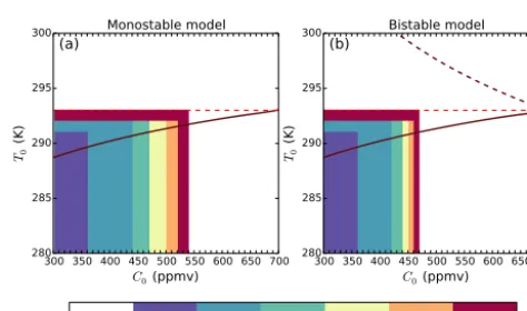
(a) (b)
Figure 2.Bifurcation diagram of the deterministic energy balance model forα1=0.45 (a; monostable model) andα1=0.2 (b; bistable model). The solid curve represents a stable equilibrium, while the dashed curve represents an unstable equilibrium.
Forσs6=0, we explicitly determine the normalized PDF p(x, t) by rewriting Eq. (6) as
dTt=f(Tt, t)dt+σsdWt, (8)
withf(T , t)=c−T1(Q0(1−α(T))+G+AlnCC(t)
ref−σ T
4), the Fokker–Planck equation of Eq. (8), which is given by
∂p ∂t +
∂(fp) ∂x −
σs2 2
∂2p
∂x2 =0. (9)
This differential equation is solved numerically for p(x, t) under any prescribed function C(t) with boundary condi-tionsp(xu, t)=p(xl, t)=0, wherexl=270 K,xu=335 K,
and an initial condition p(x,0) (specified below) satisfies Rxu
xl p(x,0)dx=1.
We first show stochastic viability kernels for each initial condition T0andC0, whereC0is an initial CO2-equivalent concentration and T0 is the expectation value of the initial PDF ofTt. As a starting time, we take the year 2030 and
sup-pose that the climate system will be forced by a certain RCP scenario from 2030 to 2200. For everyC0, the original RCP scenario from Fig. 1a is adjusted such that its time develop-ment remains the same, but it hasC0as the CO2-equivalent concentration in 2030. The PDF of the GMST p(x, t=0) (t=0 refers to the year 2030) has a prescribed variance (de-fined byσs2) and expectation valueT0.
In Fig. 3, the stochastic viability kernels are plotted for the energy balance model forced by the RCP4.5 scenario and a viable regionV defined byT ≤293 K. The results for the monostable and bistable cases are plotted in Fig. 3a and b, re-spectively. The colours indicate, for each combination ofT0 andC0, in which stochastic viability kernel the initial state (C0, T0) is located. For example, consider the bistable case and an initial condition ofT0=288 K andC0=400 ppmv; this initial condition is in the kernelVβ withβ≥0.9. This
means that, with a probability larger than 0.9, a trajectory of the model starting at (C0, T0) will remain viable up to the year 2200, whereCfollows the RCP4.5 scenario. The white areas contain initial conditions that are in a stochastic viabil-ity kernelVβ withβ <0.5.
300 350 400 450 500 550 600 650 700
C0 (ppmv) 280
285 290 295 300
T0
(K
)
(b) Bistable model
300 350 400 450 500 550 600 650 700
C0 (ppmv) 280
285 290 295 300
T0
(K
)
(a) Monostable model
0.99 0.90 0.80 0.70 0.60 0.50
Figure 3.The stochastic viability kernels for the monostable and bistable cases forced by the RCP4.5 scenario. The viable region is defined asT≤293Kand is indicated by the red dashed line. These plots show, for each combination ofT0andC0, in which stochastic viability kernel these initial values are located. The numbers in the colour bar represent theβinVβ. For convenience, the bifurcation diagram of the deterministic model is also shown.
The sensitivity of the stochastic viability kernels with re-spect to the RCP scenario, the threshold defining the viable regionV, and the amplitude of the noiseσs was also inves-tigated (results not shown). The behaviour is as expected in that the area of the kernels becomes smaller (larger) when noise is larger (smaller), when the threshold temperature is smaller (larger), and when the radiative forcing associated with the RCP scenario is more (less) severe. For example for the RCP6.0 scenario, each combination ofT0andC0(same range as in Fig. 3) is in aVβ withβ <0.5 for both
monos-table and bismonos-table cases.
3.3 Results: point of no return
Again for illustration purposes, we assume that a reduction in the emissions will have an immediate effect on the CO2eq. such that effectively the CO2eq. is controlled. We choose the collectionFλto consist of mitigation scenarios that
concentra-Table 1.Value and meaning of the parameters in the energy balance model given by Eq. (6).
cT 5.0×10⁸Jm−2K−1 Thermal inertia 1.0 Emissivity
Q0 342 Wm−2 Solar constant/4 α0 0.7 Albedo parameter
G 1.5×10²Wm−2 Constant α1 0.2 or 0.45 Albedo parameter
A 2.05×101Wm−2 Constant T0 263 K Albedo parameter
Cref 280 ppmv Reference CO2concentration T1 293 K Albedo parameter
σ 5.67×10⁻⁸Wm−2K−4 Stefan–Boltzmann constant H 0.273 K Albedo parameter
tion, which is 280 ppmv. For this exponential decay, we con-sider different e-folding timesτd. The most extreme scenario has an exponential decay within 50 years, which corresponds to an e-folding time ofτd=9 years. Hence, the collectionFλ
is given by (forτd≥9)
Fλ(t)=(Ctc−280) exp
−t−tc τd
+280. (10)
In this equation,tcis the time at which the scenario is applied,
andCtcis the associated CO2-equivalent concentration at that moment.
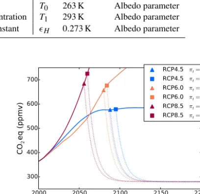
Next, we determine PNR valuesπttol for the energy bal-ance model when it is forced by the four different RCP sce-narios using a tolerance probability of βT=0.9 and a tol-erance time of τT=20 years. Theπttol values for a system forced with the RCP4.5, RCP6.0, and RCP8.5 scenarios are shown in Fig. 4 for both the monostable and bistable cases. As expected, the more extreme the RCP scenario, the earlier the PNR. This can be easily explained by the fact that when the CO2-equivalent concentration rises faster, the tempera-ture will become non-viable earlier. Consequently, the PNR will be earlier, since the GMST is only allowed to be non-viable for at mostτTyears. When the model is forced with RCP2.6, there is no PNR for either model. The reason for this is that the CO2-equivalent concentration will remain low throughout the whole period, and consequently the tempera-ture will stay viable. The value ofπttol for the bistable case is earlier than the value for the monostable case in each sce-nario. This can be clarified by the fact that the PDF of the temperature in the bistable case will leave the viable region at a lower CO2-equivalent concentration because of the exis-tence of nearby equilibria.
The sensitivity ofπttolversus the tolerance timeτTand the tolerance probabilityβTwas also investigated, and the results are as expected (and therefore not shown). A longer toler-ance time will shiftπttolto later times; for example, for the RCP4.5 scenarioπttol=2071,2088, and 2116 forτT=0,20 and 50 years for the bistable case (for fixedβT=0.9). With a fixedτT=20 years, the value ofπttolshifts to smaller values
when the tolerance probability is increased. For example, for βT=0.80 and 0.99, the values of πttol are 2127 and 2058,
respectively, for the bistable case (forβT=0.9,πttol=2088;
see Fig. 4).
2000 2050 2100 2150 2200
Year
300400 500 600 700
CO
2eq
(p
pm
v)
RCP4.5 πt=2088 RCP4.5 πt=2095 RCP6.0 πt=2080 RCP6.0 πt=2084 RCP8.5 πt=2056 RCP8.5 πt=2060
Figure 4.The PNRπttolfor a system forced with different RCP scenarios, tolerance probabilityβT=0.9, and tolerance timeτT=
te−tb=20 years. The triangles indicate the point of no return for the bistable case and the squares for the monostable case. The dotted line is the most extreme scenario ofFλwith an exponential decay to 280 ppmv and an e-folding time of 9 years. Note that for both cases there is no PNR when the model is forced with the RCP2.6 scenario.
4 PlaSim
The results in the previous section have illustrated that a PNR can be calculated when an estimate of the probability density function is available and a collection of mitigation scenarios is defined. We will now apply these concepts to the more detailed, high-dimensional climate model PlaSim, a general circulation model developed by the University of Hamburg (see https://www.mi.uni-hamburg.de/en/arbeitsgruppen/ theoretische-meteorologie/modelle/plasim.html).
us-age, and has been applied to a variety of problems in climate response theory (Ragone et al., 2016).
A main problem here is to determine a relation between the CO2eq. (and associated radiative forcing) and the GMST, i.e. a response function. Previous approaches have used a fit of a specific response function (e.g. a power law function) to available observations (Rypdal, 2016). This is more compli-cated for an approach using stochastic viability theory (ap-plying it did not produce useful results), and hence we pro-ceed by using linear response theory as described in Sect. 2.3. We use the same data as in Ragone et al. (2016) provided by F. Lunkeit and V. Lucarini (University of Hamburg, Ger-many). The difference from those in Ragone et al. (2016) is that the seasonal forcing is present, which results in a long-term increase in the GMST of 5◦C (instead of 8◦C in Ragone et al., 2016) under a scenario in which the CO2concentration doubles. The reason for this difference is not fully clear but probably results from seasonal rectification effects of nonlin-ear feedbacks. GMST data from two ensembles were used, each with 200 simulations made with two different CO2 -forcing profiles (all other GHGs are kept constant). For both forcing profiles, the starting CO2 concentration is set to a value of 360 ppmv, which is representative of the CO2 con-centration in 2000. During the first set of experiments, the CO2 concentration is instantaneously doubled to 720 ppmv and kept constant afterwards. During the second set of ex-periments, the CO2concentration increases each year by 1 % until a concentration of 720 ppmv is reached. This will take approximately 70 years, and afterwards the concentration is fixed. The total length of the simulations is 200 years. Fur-thermore, the forcingf(t) in Eq. (4) is taken as the logarithm of the CO2concentration, since the radiative forcing scales approximately logarithmically with the CO2concentration.
To determine the PDF of GMST under any CO2 -equivalent forcing, we make the assumption that at each point in time the PDF of the GMST is normally distributed. As we have 200 data points for the GMST at each time interval, aχ2 test was used to analyse the PDFs. For each time, the value of χ2>0.05 and therefore the assumption that the PDF of the GMST is normally distributed appears justified.
The Green’s functions for the expectation value and vari-ance of GMST have been calculated with the instantaneously doubling CO2profile and the associated ensemble. From the ensemble, at each point in time the expectation value and variance are calculated to obtain the temporal evolution of these two variables. Subsequently, we have found the Green’s functions using Eq. (5). To check whether these Green’s functions perform well, we compared the temporal evolution of the expectation value and variance of the GMST under the 1 % forcing (calculated with Eq. 4) with those directly gen-erated by PlaSim (Fig. 5).
The expectation value determined with LRT is close to the one directly generated by PlaSim. However, the variance of the ensemble generated by PlaSim is much noisier than the one calculated with LRT. Although the Green’s function of
the variance provides only a rough approximation, it has the right order of magnitude and we will use it to calculate the variance of the GMST for other forcing scenarios.
4.1 Results: point of no return under CO2-equivalent control
We first consider the case without a carbon cycle model, again assuming that the CO2-equivalent concentration can be controlled directly. The scenarios Fλ chosen for use in
PlaSim exponentially decay to different stabilization levels (varying between 400 and 550 ppmv; see Edenhofer et al., 2010). This stabilization level is taken as the parameterλ. We assume that stabilization happens within 100 years, which corresponds to an e-folding timeτd of about 25 years; the mitigation scenariosFλare then given by
Fλ(t)= Ctc−λ
exp−t−tc τd
+λ, (11)
wheretcis again the time at which the mitigation scenario is
applied, andCtc is the associated CO2-equivalent concentra-tion. The most extreme mitigation scenario inFλin terms of
CO2-equivalent decrease is the one that stabilizes at a CO2 -equivalent concentration of 400 ppmv.
We next determine the PNRπt2100by requiring the GMST to be viable in 2100 using a tolerance probability ofβT= 0.90. The viable region is set at T ≤16.15◦C, which cor-responds to temperatures less than 2◦C above the pre-industrial GMST.
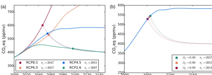
The values of πt2100 for all the RCP scenarios are plot-ted in Fig. 6a. Solid curves show the RCP scenarios, while dashed curves present the most extreme scenario Fλ. For
RCP8.5,πt2100is 10 years earlier than for RCP6.0, since the CO2-equivalent concentration increases much faster for the RCP8.5 scenario. The mitigation scenario after the point of no return, represented by the dashed line, is the same for all RCP scenarios. This is related to our definition ofπt2100, for which the GMST is required to be viable in 2100. The mitiga-tion scenario that is plotted is the ultimate scenario that guar-antees this. It indicates that for each CO2scenario the associ-atedπt2100is given by the intersection of that CO2-equivalent scenario and the mitigation scenario. This is because an ex-ponential decay to 400 ppmv within 100 years is considered always possible, no matter the CO2-equivalent concentration attc. However, when this concentration becomes too high,
this mitigation scenario is no longer very realistic.
0 50 100 150 200 Years
0.005 0.006 0.007 0.008 0.009 0.010 0.011 0.012 0.013 0.014
VA
R
(K
2)
Variance GMST
LRT PLASIM
(a) (b)
Figure 5.(a)The expectation value and(b)variance of GMST generated by PlaSim (orange) and determined through LRT (blue) for the 1 % CO2concentration increase.
2000 2050 2100 2150 2200
Year 250
300 350 400 450 500 550 600
CO2
eq
(p
pm
v)
βT=0.80 πt=2057 βT=0.90 πt=2055 βT=0.99 πt=2051
(a) (b)
Figure 6.(a)The PNRπt2100for the RCP2.6, RCP4.5, RCP6.0, and RCP8.5 scenarios for a tolerance probability ofβT=0.9 and1t=0. The solid lines represent the RCP scenarios and the dashed line the most extreme scenario fromFλ. Note that these dashed lines coin-cide.(b)The point of no return for RCP4.5 for different tolerance probabilities.
4.2 Results: point of no return under emission control Finally, we consider a more realistic case in which emis-sions are controlled and a carbon model converts emisemis-sions to CO2eq. A simple carbon model relating emissionsEto concentrationsCis given by
CCO2(t)=CCO2,0+ t Z
0
GCO2(τ)ECO2(t−τ)dτ, (12)
whereCCO2,0is the initial concentration. The Green’s func-tion for CO2is taken directly from (Joos et al., 2013):
GCO2(t)=a0+
3 X
i=1
aiet /τi, (13)
for which the parameters are shown in Table 2. The quantity ECO2 is the CO2 emission in ppm yr−1 that has been converted from ppm yr−1using the carbon molecular weight as ECO2[ppm yr−1] =γ ECO2[GtC yr−1] with γ= 0.46969 ppm GtC−1. The emissions for the RCP scenarios are taken from (Meinshausen et al., 2011) 1. The carbon model underestimates CO2levels for very high emission sce-narios as it does not include saturation of natural CO2sinks.
1See the database at http://www.pik-potsdam.de/~mmalte/rcps/
Following Table 8.SM.1 of (Myhre et al., 2013), we obtain the changes in radiative forcing compared to pre-industrial (in Wm−2) due to changes in CO2as
1FCO2=αCO2ln
CCO2
C0 , (14)
whereC0is the pre-industrial (1750) CO2concentration. We use the same PlaSim ensemble of instantaneous CO2 doubling runs again to determine a Green’s function that re-lates radiative forcing changes to temperature changes as
1T(t)=
t Z
0
GT(τ)1F(t−τ)dτ, (15)
whereGTis the data-based function determined from LRT. The total radiative forcing is taken as1F =A1FCO2, where we introduce a scaling constantAto correct for the high cli-mate sensitivity of the PlaSim model compared to typical CMIP5 models. Based on trial runs attempting to reconstruct mean CMIP5 RCP temperature trajectories with RCP CO2 emissions, we chooseA=0.6.
ex-Table 2.Model parameters. No units are given for dimensionless parameters.
CCO2,0(ppm) 278 αCO2 5.35 C0(ppm) 278
a0 0.2173 A 0.6 γ(ppm GtC−1) 0.46969
a1 0.2240 a2 0.2824 a3 0.2763
τ1(yr) 394.4 τ2(yr) 36.54 τ3(yr) 4.304
2005 2025 2045 2065 2085
Year starting to reduce emissions
1.5 2.0 2.5 3.0 3.5 4.0 4.5
9
0
%
w
ar
m
in
g
in
2
1
0
0
re
la
ti
ve
to
p
re
-i
n
d
u
st
ri
al
PLASIM warming for exponential emissions decrease (25 yr)
RCP2.6 RCP4.5 RCP6.0 RCP8.5
2000 2020 2040 2060 2080 2100
Year
350 400 450 500 550 600
CO
2
(ppm)
RCP4.5,πt= 2026
RCP6.0,πt= 2029
RCP8.5,πt= 2022
(a) (b)
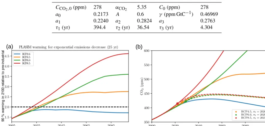
Figure 7.(a)Warming in 2100 when starting exponential CO2emission reduction in a given year.(b)CO2concentration for the four RCP scenarios as computed by the model (solid) and following exponential mitigation starting from the point of no return (dashed).
ponential:
GT(t)≈b1e−t /τb1, (16)
withb1=0.25 KW−1m2yr−1andτb1=4.69 years. We de-termine a Green’s function for the temperature variance in the same way.
To compute the point of no return πt2100 in the carbon– climate model, we start from pre-industrial CO2 concentra-tions and take the corresponding initial temperature perturba-tion as1T =0. We then prescribe the RCP emission scenar-ios for RCP2.6, RCP4.5, RCP6, and RCP8.5 (that are iden-tical up to the year 2005). At a year tb>2005 we start the
reduction in emissions at an exponential rate; i.e. fort > tb
the emissions follow
ECO2(t)=ECO2(tb) exp
−t−tb
τe
, (17)
whereτe=25 years is the e-folding timescale of the
emis-sion reduction that we keep constant. Using the carbon model, we compute the instantaneous CO2concentrations for each such scenario and use the Green’s functions for GMST mean and variance to determine the PDF in the year 2100 for each starting year tb. Assuming Gaussian distributions
(as mentioned, this is well satisfied for the original PlaSim ensemble), we can then easily determine the temperature threshold below which 90 % of the values fall. The first year for which this threshold is above 2 K givesπt2100. Note that the value of tc (in Fig. 1b), at which the CO2 starts to de-crease, is determined by the coupled carbon–climate model.
The warming in 2100 predicted by our simple climate model when starting exponential CO2emission reduction in a given year is shown in Fig. 7a. The intersections between the RCP curves (solid colour) and the dashed line (represent-ing 2 K warm(represent-ing) provide values ofπt2100. Values do not dif-fer much for the difdif-ferent RCP (4.5, 6.0, and 8.5) scenarios and are before 2030. RCP2.6 does not have a point of no re-turn as its emission scenario is sufficient to keep the warming safely below 2 K. The counter-intuitive lowering of the curve for RCP2.6 (also slightly for RCP4.5) is due to very fast emission reductions in these RCP scenarios. Starting emis-sion reduction at later times may therefore lead to lower total emissions (and hence temperatures). The CO2concentration for the four RCP scenarios as computed by the model (solid) and following the exponential mitigation starting from the point of no return (dashed) is shown in Fig. 7b. Note how emissions “still in the pipeline” lead to CO2increases even after the reduction is initiated.
5 Discussion
Pachauri et al. (2014) stated with high confidence that “with-out additional mitigation efforts beyond those in place to-day, and even with adaptation, warming by the end of the 21st century will lead to high to very high risk of severe, widespread and irreversible impacts globally”. If no mea-sures are taken to reduce GHG emissions during this century and if there are no new technological developments that can reduce GHGs in the atmosphere, it is likely that the GMST will be 4◦C higher than the pre-industrial GMST at the end of the 21st century (Pachauri et al., 2014). Consequently, it is important that anthropogenic emissions are regulated and significantly reduced before widespread and irreversible im-pacts occur. It would help motivate mitigation to know when it is “too late”.
In this study we have defined the concept of the point of no return (PNR) in climate change more precisely using stochas-tic viability theory and a collection of mitigation scenarios. For an energy balance model, as in Sect. 3, the probabil-ity densprobabil-ity function could be explicitly computed, and hence stochastic viability kernels could be determined. The addi-tional advantage of this model is that a bistable regime can easily be constructed to investigate the effects of tipping be-haviour on the PNR. We used this model (with the assump-tion that CO2could be controlled directly instead of through emissions) to illustrate the concept of PNR based on a toler-ance time for which the climate state is non-viable. For the RCP scenarios considered, the PNR is smaller in the bistable than in the monostable regime of this model. The occurrence of possible transitions to warm states in this model indeed cause the PNR to be “too late” earlier.
The determination of the PNR in the high-dimensional PlaSim climate model, however, shows the key innovation in our approach, i.e. the use of linear response theory (LRT) to estimate the probability density function of the GMST. PlaSim was used to compute another variant of a PNR based only on the requirement that the climate state is viable in the year 2100. Hence, the PNR here is the time at which no allowed mitigation scenario can be chosen to keep GMST below a certain threshold in the year 2100 with a specified probability. In the PlaSim results, we used a viability region defined as GMSTs lower than 2◦C above the pre-industrial value, but with our methodology, the PNR can be easily de-termined for any threshold defining the viable region. The more academic case in which we assume that GHG levels can be controlled directly provides PNR (for RCP4.5, RCP6.0, and RCP8.5) values around 2050 (Sect. 4.2). However, the more realistic case in which the emissions are controlled (Sect. 4.3) and a carbon model is used reduces the PNR for these three RCP scenarios by about 30 years. The reason is that there is a delay between the decrease in GHG gas emis-sions and concentrations.
Although our approach provides new insights into the PNR in climate change, we recognize that there is potential
for substantial further improvement. First of all, the PlaSim model has a too-high climate sensitivity compared to CMIP5 models. Although in the most realistic case (Sect. 4.3) we somehow compensate for this effect, it would be much better to apply the LRT approach to CMIP5 simulations. Second, in the LRT approach, we assume the GMST distributions to be Gaussian. This is well justified in PlaSim, as can be verified from the PlaSim simulations, but it may not be the case for a typical CMIP5 model. Third, for the more realistic case in Sect. 4.3, we do not capture the uncertainties in the carbon model and hence in the radiative forcing.
A large ensemble such as that available for PlaSim is not available (yet) for any CMIP5 model. However, we have re-cently applied the same methodology to two CMIP5 model ensembles, i.e. a 34-member ensemble of abrupt CO2 qua-drupling and a 35-member ensemble of smooth 1 % CO2 in-crease per year. The CO2-quadrupling ensemble was used to derive the Green’s function, and then the 1 % CO2 in-crease ensemble was used as a check on the resulting re-sponse. The probability density function of GMST increase is close to Gaussian for the 1 % CO2increase ensemble but clearly deviates from a Gaussian distribution for the 4x CO2 -forcing ensemble, particularly at later times. Although the ensemble is relatively small and the models within the en-semble are different (but many are related), the results for the LRT-determined GMST response (Aengenheyster, 2017) are surprisingly good. This indicates that the methodology has a high potential to be successfully applied to the results of CMIP5 model simulations (and in the future, CMIP6). The applicability of LRT to other observables than GMST can in principle be performed, but the results may be less useful (e.g. due to non-Gaussian distributions).
Because PlaSim is highly idealized compared to a typ-ical CMIP5 model, one cannot attribute much importance to the precise PNR values obtained for the PlaSim model as in Fig. 7. However, we think that our approach is gen-eral enough to handle many different political and socio-economic scenarios combined with state-of-the-art climate models when adequate response functions of CMIP5 mod-els have been determined (e.g. using LRT). Hence, it will be possible to make better estimates of the PNR for the real climate system. We therefore hope that these ideas on the PNR in climate change will eventually become part of the decision-making process during future discussions about cli-mate change.
Data availability. Data are now available via https://doi.org/10.5281/zenodo.838675 (Van Zalinge et al., 2017).
Acknowledgements. This study was supported by the MC-ETN CRITICS project. We thank Valerio Lucarini and Frank Lunkeit (University of Hamburg) for providing the PlaSim model data. We thank the reviewers for the critical, excellent, and stimulating comments which improved the paper substantially.
Edited by: Christian Franzke
Reviewed by: Kristoffer Rypdal, Jobst Heitzig, and two anonymous referees
References
Aengenheyster, M.: Point of No Return and Optimal Transitions in CMIP5, Faculty of Science Theses (Master thesis), Utrecht Uni-versity archive, available at: https://dspace.library.uu.nl/handle/ 1874/351607, 2017.
Aubin, J.-P.: Viability theory, Springer Science & Business Media, New York, 2009.
Budyko, M.: Effect of solar radiation variation on climate of Earth, Tellus, 21, 611–619, 1969.
Doyen, L. and De Lara, M.: Stochastic viability and dynamic pro-gramming, Syst. Control Lett., 59, 629–634, 2010.
Edenhofer, O., Knopf, B., Barker, T., Baumstark, L., Bellevrat, E., Chateau, B., Criqui, P., Isaac, M., Kitous, A., Kypreos, S., and Leimbach, M.: The economics of low stabilization: model com-parison of mitigation strategies and costs, Energ. J., 31, 11–48, 2010.
Fraedrich, K., Jansen, H., Kirk, E., Luksch, U., and Lunkeit, F.: The Planet Simulator: Towards a user friendly model, Meteorol. Z., 14, 299–304, 2005.
Hansen, J., Sato, M., Kharecha, P., Beerling, D., Berner, R., Masson-Delmotte, V., Pagani, M., Raymo, M., Royer, D. L., and Zachos, J. C.: Target atmospheric CO2: Where should human-ity aim?, The Open Atmospheric Science Journal, 2, 217–231, https://doi.org/10.2174/1874282300802010217, 2008.
Heitzig, J., Kittel, T., Donges, J. F., and Molkenthin, N.: Topol-ogy of sustainable management of dynamical systems with de-sirable states: from defining planetary boundaries to safe oper-ating spaces in the Earth system, Earth Syst. Dynam., 7, 21–50, https://doi.org/10.5194/esd-7-21-2016, 2016.
Hogg, A. M.: Glacial cycles and carbon dioxide: A
conceptual model, Geophys. Res. Lett., 35, L01701, https://doi.org/10.1029/2007GL032071, 2008.
Joos, F., Roth, R., Fuglestvedt, J. S., Peters, G. P., Enting, I. G., von Bloh, W., Brovkin, V., Burke, E. J., Eby, M., Edwards, N. R., Friedrich, T., Frölicher, T. L., Halloran, P. R., Holden, P. B., Jones, C., Kleinen, T., Mackenzie, F. T., Matsumoto, K., Meinshausen, M., Plattner, G.-K., Reisinger, A., Segschneider, J., Shaffer, G., Steinacher, M., Strassmann, K., Tanaka, K., Tmermann, A., and Weaver, A. J.: Carbon dioxide and climate im-pulse response functions for the computation of greenhouse gas metrics: a multi-model analysis, Atmos. Chem. Phys., 13, 2793– 2825, https://doi.org/10.5194/acp-13-2793-2013, 2013.
Mann, M. E.: Defining dangerous anthropogenic interference, P. Natl. Acad. Sci. USA, 106, 4065–4066, 2009.
Meinshausen, M., Smith, S. J., Calvin, K., Daniel, J. S., Kainuma, M. L. T., Lamarque, J.-F., Matsumoto, K., Montzka, S. A., Raper, S. C. B., Riahi, K., Thomson, A., Velders, G. J. M., and van Vu-uren, D. P.: The RCP greenhouse gas concentrations and their extensions from 1765 to 2300, Climatic Change, 109, 213–241, https://doi.org/10.1007/s10584-011-0156-z, 2011.
Myhre, G., Shindell, D., Bréon, F.-M., Collins, W., Fuglestvedt, J., Huang, J., Koch, D., Lamarque, J.-F., Lee, D., Mendoza, B., Nakajima, T., Robock, A., Stephens, T., Takemura, T., and Zhang, H.: Anthropogenic and Natural Radiative Forcing Sup-plementary Material, in: Climate Change 2013 – The Physi-cal Science Basis, edited by: Jacob, D., Ravishankara, A. R., and Shine, K., chap. 8, Cambridge University Press, Cambridge, 2013.
Pachauri, R. K., Allen, M. R., Barros, V. R., Broome, J., Cramer, W., Christ, R., Church, J. A., Clarke, L., Dahe, Q., Dasgupta, P., and Dubash, N. K.: Climate Change 2014: Synthesis Report. Contribution of Working Groups I, II and III to the Fifth Assess-ment Report of the IntergovernAssess-mental Panel on Climate Change, 2014.
Petschel-Held, G., Schellnhuber, H. J., Bruckner, T., Tóth, F. L., and Hasselmann, K.: The Tolerable Windows Approach: Theo-retical and Methodological Foundations, Climatic Change, 41, 303–331, 1999.
Ragone, F., Lucarini, V., and Lunkeit, F.: A new framework for cli-mate sensitivity and prediction: a modelling perspective, Clim. Dynam., 46, 1459–1471, 2016.
Ragone, F., Lucarini, V., and Lunkeit, F.: A new framework for climate sensitivity and prediction: a modelling perspective, Clim. Dynam., 46, 1459–1471, https://doi.org/10.1007/s00382-015-2657-3, 2016.
Rogelj, J., Hare, W., Lowe, J., van Vuuren, D. P., Riahi, K., Matthews, B., Hanaoka, T., Jiang, K., and Meinshausen, M.: Emission pathways consistent with a 2◦C global temperature limit, Nature Publishing Group, 1, 413–418, 2011.
Rypdal, K.: Global warming projections derived from an observation-based minimal model, Earth Syst. Dynam., 7, 51– 70, https://doi.org/10.5194/esd-7-51-2016, 2016.
Sellers, W. D.: A global climatic model based on the energy balance of the earth-atmosphere system, J. Appl. Meteorol., 8, 392–400, 1969.
Smith, J. B., Schneider, S. H., Oppenheimer, M., Yohe, G. W., Hare, W., Mastrandrea, M. D., Patwardhan, A., Burton, I., Corfee-Morlot, J., Magadza, C. H., and Füssel, H. M.: Assessing danger-ous climate change through an update of the Intergovernmental Panel on Climate Change (IPCC) “reasons for concern”, P. Natl. Acad. Sci. USA, 106, 4133–4137, 2009.
Van Zalinge, B., Feng, Q. Y., Aengenheyster, M., and Dijkstra, H. A.: PNRESD: Data for “On determining the point of no return in climate change”, https://doi.org/10.5281/zenodo.838675, 3 Au-gust 2017.