Atmos. Meas. Tech., 6, 1761–1776, 2013 www.atmos-meas-tech.net/6/1761/2013/ doi:10.5194/amt-6-1761-2013
© Author(s) 2013. CC Attribution 3.0 License.
EGU Journal Logos (RGB)
Advances in
Geosciences
Open Access
Natural Hazards
and Earth System
Sciences
Open AccessAnnales
Geophysicae
Open AccessNonlinear Processes
in Geophysics
Open AccessAtmospheric
Chemistry
and Physics
Open AccessAtmospheric
Chemistry
and Physics
Open Access DiscussionsAtmospheric
Measurement
Techniques
Open AccessAtmospheric
Measurement
Techniques
Open Access DiscussionsBiogeosciences
Open Access Open Access
Biogeosciences
Discussions
Climate
of the Past
Open Access Open Access
Climate
of the Past
Discussions
Earth System
Dynamics
Open Access Open Access
Earth System
Dynamics
DiscussionsGeoscientific
Instrumentation
Methods and
Data Systems
Open Access
Geoscientific
Instrumentation
Methods and
Data Systems
Open Access DiscussionsGeoscientific
Model Development
Open Access Open Access
Geoscientific
Model Development
DiscussionsHydrology and
Earth System
Sciences
Open AccessHydrology and
Earth System
Sciences
Open Access DiscussionsOcean Science
Open Access Open Access
Ocean Science
DiscussionsSolid Earth
Open Access Open Access
Solid Earth
DiscussionsThe Cryosphere
Open Access Open Access
The Cryosphere
Discussions
Natural Hazards
and Earth System
Sciences
Open Access
Discussions
Calibration and validation of the advanced E-Region Wind
Interferometer
S. K. Kristoffersen1, W. E. Ward1, S. Brown2, and J. R. Drummond3
1Department of Physics, University of New Brunswick, Fredericton, NB, E3B 5A3, Canada
2CRESS Space Instrumentation Laboratory CSIL, York University, 4700 Keele St. Toronto, ON, M3J 1P3, Canada 3Department of Physics and Atmospheric Science, Dalhousie University, Halifax, NS, B3H 4R2, Canada
Correspondence to: W. E. Ward ([email protected])
Received: 31 October 2012 – Published in Atmos. Meas. Tech. Discuss.: 14 November 2012 Revised: 8 March 2013 – Accepted: 31 March 2013 – Published: 23 July 2013
Abstract. The advanced E-Region Wind Interferometer (ER-WIN II) combines the imaging capabilities of a CCD detector with the wide field associated with field-widened Michelson interferometry. This instrument is capable of simultaneous multi-directional wind observations for three different air-glow emissions (oxygen green line (O(1S)) at a height of ∼97 km, thePQ(7) andPP(7) emission lines in the O2(0–1) atmospheric band at∼93 km and P1(3) emission line in the (6, 2) hydroxyl Meinel band at∼87 km) on a three minute cadence. In each direction, for 45 s measurements for typical airglow volume emission rates, the instrument is capable of line-of-sight wind precisions of∼1 m s−1for hydroxyl and O(1S) and∼4 m s−1for O
2. This precision is achieved using a new data analysis algorithm which takes advantage of the imaging capabilities of the CCD detector along with knowl-edge of the instrument phase variation as a function of pixel location across the detector. This instrument is currently lo-cated in Eureka, Nunavut as part of the Polar Environment Atmospheric Research Laboratory (PEARL) (80◦N, 86◦W). The details of the physical configuration, the data analysis algorithm, the measurement calibration and validation of the observations from December 2008 and January 2009 are de-scribed. Field measurements which demonstrate the capabil-ities of this instrument are presented. To our knowledge, the wind determinations with this instrument are the most accu-rate and have the highest observational cadence for airglow wind observations of this region of the atmosphere and match the capabilities of other wind-measuring techniques.
1 Introduction
Interferometric methods have been used for the past thirty years to passively observe mesospheric and thermospheric winds using Doppler shifts in airglow emissions. Progress in detector technologies have led to advances in the observation capabilities of these instruments by allowing the interference fringes and/or the scene of interest to be imaged. Apart from the Wind Imaging Interferometer (WINDII) on the Upper At-mosphere Research Satellite (Shepherd et al., 1993), publica-tions on working instruments have generally been associated with the Fabry–Perot (Aruhliah et al., 2010; Anderson et al., 2012; Shiokawa et al., 2012) and spatial heterodyne spec-troscopy (SHS) techniques (the Doppler Asymmetric Spatial Heterodyne – DASH – of Englert et al., 2012). The success of these instruments demonstrates how incorporating imag-ing capabilities improves the accuracy and temporal resolu-tion over earlier configuraresolu-tions.
at 557.7 nm, thePP(7) andPQ(7) lines in the O2(0–1) atmo-spheric band at 865.9 and 866.1 nm and the P1(3) emission line in the OH(6,2) Meinel band at 843.0 nm) every three minutes. The wind accuracy is∼1 m s−1 for all the emis-sions and the precision is∼1 m s−1 for the green-line and hydroxyl observations and∼4 m s−1for the O2observations for standard operating conditions.
ERWIN II is based on the E-region wind interferometer (Gault et al., 1996) which was built in the mid-1990s using a photomultiplier tube as a detector. Winds were obtained by sequentially viewing different directions. This instrument was stationed at Resolute Bay for close to a decade and sev-eral papers on the associated observations published (Fisher et al., 2000, 2002; Bhattacharya and Gerrard, 2010).
In 2005, funding through a Canadian Foundation of Inno-vation grant became available and was used to design and build an improved version of the instrument. The interferom-eter and filters from the old version of the instrument were retained but the optical configuration and imaging detectors were new. The imaging capability allowed a new data anal-ysis algorithm to be developed, which improved the accu-racy and precision of the instrument. Once completed, ER-WIN II was moved to the Polar Environment Atmospheric Research Laboratory (PEARL) in Eureka, Nunavut (80◦N, 86◦W) in February 2008. It operated satisfactorily for three winters till spring 2011, when some minor issues with its op-eration occurred. These have been fixed and normal opera-tions resumed in the winter of 2012/2013.
This paper is organized as follows. The next two sections deal with concepts and details necessary for understanding the instrument namely the measurement and instrument con-cept, and a description of the new instrument and its op-eration. In the subsequent section, the data analysis algo-rithms are described. A section on the precision and ac-curacy of these measurements and their validation follows this. Some initial results along with a comparison with other wind-measuring instruments and a brief review summary of the planned scientific studies with this instrument are then presented. The paper finishes with some concluding remarks.
2 Measurement and instrument concept
Doppler shifts in isolated quasi-monochromatic emissions when viewed through an ideal Michelson interferometer are seen as changes in the modulation of the interference fringes as a function of path difference. The measured irradiance I (1, λ, x)for an isolated monochromatic emission line has the following form:
I (1, λ, x)=I0
1+U V cos 2
π λ 1+x
+IB. (1) HereI0is the irradiance of the emission alone as measured at the detector in the absence of interference,1is the path difference of the interferometer,λis the wavelength of the
emission,xrepresents small variations in path (typically less thanλ) that the experimenter can introduce into the inter-ferometer to sample a fringe,U is the relative reduction in fringe amplitude due to instrument effects,V is the relative reduction in fringe amplitude due to the finite width of the emission line and the path difference, andIBis the sum of the background irradiance of the scene being viewed and de-tector dark count processes.
The phase,θ, of the fringe is defined as 2πλ 1. A small change in wavelength due to a Doppler shift, λ+δ λ, re-sults in a change in phase of δθ=−2π
λ2
1 δ λ plus a small correction associated with the dispersion of the glass. For small line-of-sight velocities, vlos, the Doppler shift is δ λ=−λ (vlos/c)with positive line-of-sight velocities corre-sponding to a velocity towards the observer. Hence, the phase change associated with this Doppler shift is
δθ = 2π 1 vlos
c λ . (2)
Observation of the phase shift relative to the zero-wind phase allows the line-of-sight velocity to be derived.
As described in detail elsewhere (Shepherd, 2002), Doppler Michelson interferometry determines winds by de-termining phase shifts in the interference by measuring the irradiance passing through the interferometer at specific path differences and determining the fringe parameters from these measurements. Typically, the interferometer path is varied in phase steps of 90 degrees of phase. The standard 4-point al-gorithm (for ideal conditions: no background or dark count) uses irradiance measurements at four such sequential steps to derive the fringe parameters (irradiance, visibility and phase) as follows:
I0 =
I1+I2+I3+I4 4
U V =
(I1−I3)2+(I4−I2)21/2
2I0 θa =tan−1
I4−I2 I1−I3
. (3)
one of the arms of the interferometer and positioning the mir-ror in the other arm at the apparent position of the mirmir-ror of the arm with the excess glass in it so that the conditions when the arms are the exactly the same are approximately achieved. This configuration eliminates the second-order de-pendence of path as a function of angle and can eliminate the fourth-order dependence for specific mirror positions (Zwick and Shepherd, 1971).
The precision of a wind measurement is basically related to how well the sinusoidal variation associated with a varia-tion in path can be discerned relative to the inherent noise as-sociated with that measurement. For a shot-noise-limited ob-servation, a reasonable estimate of accuracy of the phase de-termination is the standard deviation inθ,σθ, which is given by Ward (1988):
σθ = 1 a U V√I0
, (4)
whereais a constant which depends on the number of steps used to determine the fringe phase. For the four point mea-surement described abovea=√2. For the 8-step scans used for ERWIN II,a= 2.
The two fringe-related parameters in this equation are the net visibility,U V, and√I0, which is the signal-to-noise ra-tio. In practice, the measurement precision can be increased by increasing the signal (longer integration times and en-hanced instrument responsivity) or the visibility. The visi-bility is determined by the emission line width, background emissions, the instrument imperfections and the phase vari-ation over the region used to detect the light (essentially the aperture effect discussed by Hilliard and Shepherd, 1966).
Contributions of background or dark signal to the observed irradiance also affect the measurement precision. In terms of the above formulation for ideal conditions, this can be ac-commodated by determining effective irradiances and effec-tive visibilities where the effeceffec-tive irradiance isI0e=I0+IB and the effective visibility isU Ve=U V (I0/ (I0+IB)). In the rest of this paper, for simplicity, expressions will be pro-vided for the ideal conditions (i.e. no dark and no back-ground) with the understanding that for non-ideal conditions, the effective irradiance and visibility can be used without any change to their form.
The wind accuracy is a function of both the measure-ment precision and knowledge of the phase for a stationary source, termed here the zero-wind phase. Generally, practi-cal sources for the airglow emissions are not available so the zero-wind phase is determined by using lamps with emis-sion lines at wavelengths close to the airglow emisemis-sions and using nightly averages of the wind in the vertical direction under the assumption that vertical motions average to a value smaller than the precision.
3 Instrument description and operation
ERWIN II differs from the original instrument in that the photomultiplier tube was replaced by an imaging detector, the optics were modified so that light from the four cardinal directions and the vertical could be viewed simultaneously, and the interferometer was placed in an air-tight housing to prevent pressure changes associated with weather fronts from affecting the phase. The interferometer, airglow emissions, calibration lines and the filters used are the same as ERWIN and are described in detail in Gault et al. (1996).
In summary, the interferometer is a three-glass design with the mirror position controlled using piezoelectric cylinders and a capacitive feedback system. The front face is square with sides of 7.62 cm. It was designed to accept a beam with a 2.5◦ half angle. The interferometer is set to a path
difference slightly larger than 11 cm and the glass lengths were chosen so that the interferometer is field widened at all wavelengths and thermally compensated. The specific path difference was selected to suppress possible fringes from thermospheric oxygen green-line emissions, and to ensure the fringes of the pair of O2 lines and the 3doubled hy-droxyl lines were each in phase. The calibration lines used are the 557.0 nm krypton line, the 840.8 nm argon line and the 866.7 nm argon line.
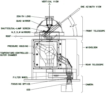
Figure 1 is a schematic view of the mechanical layout of ERWIN II. It shows a cut through the centre of the instru-ment such that two of the cardinal viewing directions and the vertical can be seen (the other viewing directions project out of the plane of the figure). The centres of each cardinal view-ing direction are at an elevation angle of 38.7◦relative to the
horizontal. Light from the sky from all the viewing directions is collected and focused on what is termed the quad mirror, where they are combined into a single beam and then passed through the interferometer. The interferometer is tilted 1.77◦ horizontally and 1.77◦vertically relative to the optical axis of the system to ensure that no light was reflected off opti-cal components and recycled back through the system. The optical components which collect the light and collimate it through the interferometer form what is termed the front tele-scope. After the interferometer, a second optical system – termed the back telescope – directs the light to the filters, where the light is again collimated. Both telescopes are 1 : 1. The camera system then focuses the beam onto the detector. The calibration lamps are located outside of the Michelson housing and are not pictured in the schematic shown in Fig. 1. The lamps are connected to fibre optic cables, which are di-rected at the calibration lamp screen. This screen acts as a shutter; when it is closed, atmospheric measurements cannot be taken. To take calibration lamp measurements, this shut-ter/screen is closed, and illuminated by the calibration lamps, and thereby acting as a source for the calibration lines.
Fig. 1. Diagram of ERWIN mechanical layout.
combine with the zenith light into a single beam through the rest of the optical system. Each of the cardinal directions views an irregularly shaped piece of the sky approximately 0.0013 steradians at an elevation angle of 38.7◦. Zenith is viewed with a solid angle of 0.0007 steradians. Light from each of the cardinal directions is focused onto one of the trapezoidal facets of the quad mirror using spherical mirrors and zenith is focused onto the plane of this mirror. The quad mirror is located at the field stop of the front telescope. The light from these various viewing directions is passed as col-limated light through the interferometer and then focused us-ing a second telescope and camera onto the detector. The sky from each direction is thus focused onto different regions of the detector so that each of these five directions is simultane-ously measured. The effective field of view of the instrument
is the same as that allowed through the interferometer – a beam of 2.5◦half angle.
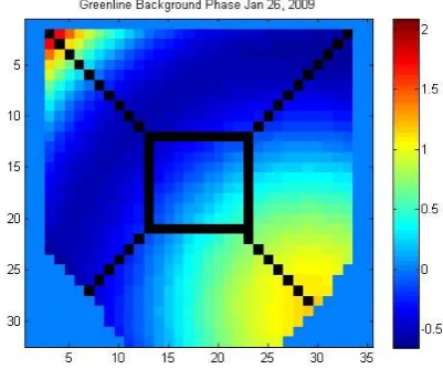
Fig. 2. Green-line background phase (in radians) from 26 Jan-uary 2009. The x- and y-axes represent pixel indices. The blackened bins represent the borders between the sections of the quad mirror. The top section measures east, the bottom, west, the left, south, the right, north, and the centre zenith.
comparable signal to noise. For ERWIN II the radiance response is 1.7672 Rayleigh (counts s)−1 for green line, 2.0682 Rayleigh (counts s)−1 for O2 and 1.0627 Rayleigh (counts s)−1for OH.
Figure 2 illustrates the manner in which the field is im-aged onto the CCD detector. The dark bins indicate where the edges of the areas illuminated by the various regions of the sky are located. The light from each viewing direction is imaged as follows: the top – east, the bottom – west, the right – north, the left – south, and the centre – zenith. The background colours indicate how the interferometer phase in radians varies across the field and indicate how much vari-ation there is across each region. Varivari-ations in phase away from this background along with consideration of the zero wind provide a measure of the Doppler shift in each viewing direction.
The observation procedure of ERWIN II has been updated relative to that described in Gault et al. (1996). Since all viewing directions are now viewed simultaneously, there is no need to cycle through the viewing directions. The basic procedure is to cycle through the three emission measure-ments in sequence and then after a user specified number of cycles to perform a set of calibrations. A measurement con-sists of 8 exposures of the detector each at a different value of the Michelson path. The steps (relative to the reference phase which coincides with the initial mirror position) are set to 0, 90, 180, 270, 270, 180, 90 and 0◦of phase. These steps are different for each emission with 360◦corresponding to a physical change in path ofλ, the wavelength of the emission being viewed. A calibration consists of measurements (again one for each emission) using the calibration lamps and a dark measurement. Initially, a calibration was undertaken after ev-ery eight emission scans, but later this was changed to evev-ery
Fig. 3. Schematic of the viewing geometry of ERWIN II. This shows three fields of view. The other two are orthogonal to the plane of the page.
set of emission scans to provide better precision for deter-mining the interferometer drift. Overall, this results in a set of observations (wind determinations for 5 directions and all three emissions) approximately every 3 min. ERWIN takes measurements as long as the solar elevation is less than 0◦.
The observing geometry is illustrated in Fig. 3. All three emission layers are shown schematically and occur roughly at nominal heights of 97, 93 and 87 km for the O(1S), O
2 and OH emissions, respectively. Thus, by cycling through the different emissions, information on various heights in the mesopause region is acquired. The azimuthal viewing direc-tions are at an elevation angle ofα= 38.7◦from the horizon-tal. Based on this observing geometry, the∼5◦lateral cross section of each beam, and a mean height of 90 km and a nom-inal vertical scale of∼5 km for the half width of the airglow layer, the volume of atmosphere sampled by ERWIN II is ∼5 km in the vertical and 5km by 6km in the horizontal. (It will not be sensitive to vertical scales less than approximately half the thickness of the airglow layer –∼5 km). Since winds are determined by observing Doppler shifts in the emission frequencies, the observed, line-of-sight winds are combina-tions of the horizontal and vertical winds (save for the zenith line-of-sight winds, which observe vertical winds).
The meridional wind,v, is determined using the difference of the line-of-sight north and south winds
v = V LOS
S −V
LOS N
2 cosα , (5)
where
VNLOS = −vcosα+wsinα (6)
VSLOS =vcosα+wsinα. (7)
Similarly, the zonal wind,u, can be determined using the east and west line-of-sight winds,
u= V LOS
W −V
LOS E
2 cosα . (8)
The vertical winds can also be obtained using several differ-ent approaches. The most precise and accurate is to use the zenith line-of-sight winds
w=VZLOS. (9)
The vertical winds can be also be determined indirectly using the cardinal direction line-of-sight winds,
w= V LOS
N +VSLOS 2 sinα =
VELOS+VWLOS
2 sinα . (10)
In theory, this provides the means to check the internal con-sistency of the wind determinations, but only for longer tem-poral scales. In practice, the effects of gravity waves of scales of the same order as the distance between the viewing points (∼250 km) in the airglow layer will result in oppositely di-rected fields of view measuring winds that differ as a re-sult of the aliasing of wind variations associated with these waves. This means that these comparisons can only be un-dertaken for longer term averages for which the spatial scales are significantly larger than 250 km. At the same time these shorter term differences between opposing fields of view al-low observations of gravity wave effects to be undertaken, given confidence in the instrument calibration. This will be described in detail in a forthcoming paper.
4 Data analysis procedure
The essential issue for wind measurements is distinguishing the phase increments,δ θ, associated with Doppler shifts in the emission of interest from the phase associated with other factors. In general, the observed phase is a combination of the phase associated with the instrument configuration as mani-fested for the emission of interest (motionless) plus a shift associated with atmospheric motion of the source region be-ing viewed. In practice, for imagbe-ing applications, the phase associated with the instrument configuration can be separated into three terms:
– θB(i, j ): a term associated with the phase variation across the field as a function of angle through the inter-ferometer (or pixel location (i, j) on the detector) rel-ative to the phase associated with rays passing at nor-mal incidence through the interferometer (background phase). This variation is illustrated in Fig. 2.
– θT(t ):a term giving the thermal-drift phase of the inter-ferometer relative to the phase observed at a particular time (thermal-drift term).
– θ0: a term identifying the phase that a motionless source would have (zero-wind phase).
Hence, the measured phase,θa, can be expressed as a func-tion of time,t, and location on the field as
θa(i, j, t )=θB(i, j )+θ0+θT(t )+δ θ (t ). (11) This formulation of the phase assumes that the back-ground phase stays constant (generally satisfied for carefully maintained interferometers) and temporal variations can be tracked with a single phase parameter, the thermal drift, which is only a function of time.
In theory, the zero-wind phase should be easy to determine since it only requires a stationary source for the emission of interest. In practice, however, this is difficult to achieve since portable sources for the airglow emissions are unavailable and the atmosphere is generally in motion. As with other ground-based wind instruments, a daily average of the ob-served vertical wind is used to determine this parameter. In the case of ERWIN II this average is measured using the quadrant looking vertical. For measurements at Eureka, where close to 24 h each day is observed, this determination is expected to be a good measure of the actual zero wind; all periods of tidal motions are covered during this time pe-riod, variations associated with gravity waves are expected to average to zero, vertical winds associated with planetary waves are of the order of cm s−1and mean vertical winds are small (an ascent or descent of 10 km day−1corresponds to a vertical velocity of 0.11 m s−1).
For ERWIN II the background phase determination was more difficult than expected. Initially, it was thought the phase variation associated with the reference emissions would be suitable to use since they were within a few
˚
Angstr¨oms of the emission of interest. However, it was found that use of such a background resulted in phase variations of ∼10 m s−1 across several of the quadrants when daily av-erages of the winds were calculated. This effect is thought to be due to differences between the calibration optics and main optics which result in the light distribution across the aperture of each system being different and resulting in a different weighting of any residual path variations in the in-terferometer. Instead, the background phase which was used was determined using wind observations from a period when it was known to be cloudy (this phase variation is illustrated in Fig. 2 for the green line). Light from the sky was suit-ably scattered so that all directions gave the same Doppler shift. Daily averages of this wind for the oxygen green-line and hydroxyl observations using this background are pre-sented in Fig. 4. The resulting wind variations are minimal in each quadrant and the mean wind in each quadrant pro-vides a measure of the mean wind for the day. Details of the analysis which lead to this choice of background wind are contained in Kristoffersen (2012).
the signal in each quadrant and treating each quadrant as a single detector, a new bin-by-bin least-mean-squares ap-proach similar to that implemented in Ward (1988) was pre-ferred. The latter approach was more precise since it avoids any visibility reduction that occurs as a result of the inte-gration over the phase in each quadrant, and it allows bins contaminated by stars or cosmic ray hits to be eliminated. In addition, a rigorous determination of the wind error can be undertaken.
For this approach, a non-linear least-mean-squares analy-sis using the Levenberg Marquardt method (as described in Press et al., 2007) is implemented. The variation in photons detected per integration time for a step during thek-th 8-point scan is modelled according to the following equation: I (i, j, tk, s)=I0(tk) (1+U V (tk)cos(δ θ (tk)+θI(i, j, tk, s))) , (12) where the parameters being solved for areI0(tk), the num-ber of photons detected per integration time for a step in the absence of interference,U V (tk), the net visibility, and δ θ (tk), the phase variation associated with the wind. Here tk is the time of thek-th scan. To ensure that the variation in angles being determined is small, all the known phases associated with a particular bin are added together so that θI(i, j, tk, s)=θB(i, j )+θ0+θT(tk)+(1 θs), where(1 θs) is the step size increment associated with mirror step of in-dex s (expressed as a phase angle).
The merit function is
χ2= N X
s=1
Is(i, j, tk, s)−y (I (i, j, tk, s); al) 2
σ2
s (i, j, tk, s)
, (13)
where
y (I (i, j, tk, s); al)=al(1) (1+al(2)cos(al(3)+θI(i, j, tk, s)))
al = I0l(tk) , U Vl(tk) , δ θl(tk)
.
Is(i, j, tk, s)is the number of photons detected for stepss, bin (i, j) and scank, andσs2(i, j, tk, s)is the associated vari-ance (estimated as shot noise). l is the iteration index, so y (I (i, j, tk, s); al)is the number of photons detected de-termined using the constants dede-termined on thel-th iteration. θI(i, j, tk, s)with1 θs= 0 is used to seed the first iteration of this method. Typically, only a few iterations are needed for convergence to a solution.
In practice, there are two approaches used to determine the zero wind and thermal-drift phase: one using the calibration lamp phase determinations (the standard procedure) and the other when the calibration lamp phase is not available (as oc-curred for the OH emission when the lamp malfunctioned). For the standard procedure, the calibration phase was deter-mined on a regular basis throughout the night by calculating the average Michelson phase over the full field of the cali-bration lamp using the same 8-point scan as for the airglow observations. The resulting time series of calibration phase is interpolated using cubic splines to the airglow observation
times to provide the variation in the thermal-drift phase. The relative airglow phase throughout the observation period is then calculated using the non-linear approach with the zero-wind phase set to zero. The actual zero-zero-wind phase then pro-vides an offset to this relative phase and is determined using the mean of the zenith over the entire day. The winds are de-termined by shifting the relative airglow phase by the zero-wind phase and using Eq. (2) to convert the phase to velocity. If the calibration lamps are not available, then the zenith measurements can be used to estimate the phase associated with the thermal drift and zero wind. In this case, the anal-ysis approach as described above is undertaken but with the thermal-drift and zero-wind terms set to zero. For each im-age, the phase for the vertical view is then taken as an esti-mate of the sum of these two terms and subtracted off the four other quadrants. The disadvantage of this approach is that the vertical wind cannot be determined and phase variations as-sociated with vertical winds are mixed into the phase deter-minations for each of the cardinal directions. This reduces the precision and accuracy of the radial wind determination. Nevertheless, the meridional and zonal wind determinations are unaffected by the lack of an independent zero-wind de-termination since they are determined through a difference in radial wind determinations in opposite directions, and hence the zero-wind contribution to the two directions is eliminated (see Eqs. 5 and 8).
There are several advantages associated with the standard approach described above. This algorithm can be run for fewer than the 8 steps comprising a typical scan. Because the steps are in phase multiples of 90◦and all phases steps are repeated twice, anomalous numbers of photons detected at a particular step can be identified by comparing photon num-bers observed for steps of the same phase and examining the sums of photon numbers for steps which are 180◦ apart. If one or two steps with anomalous numbers of detected pho-tons are identified in a scan, they are eliminated from the phase determination, thereby reducing the likelihood of out-liers. In addition, there are∼150 bins used for wind deter-minations in each of the cardinal directions and ∼80 bins for the vertical. As a result, any additional outliers beyond three standard deviations of the mean wind phase in each of the quadrants can be identified and are then eliminated and the standard error associated with the wind determination for each quadrant calculated. Implementation of these checks re-sults in a robust statistical framework for the wind determi-nations with this instrument.
5 Measurement validation
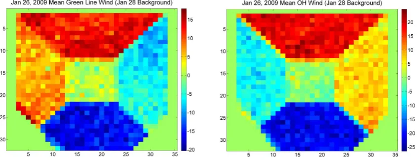
Fig. 4. An image of the daily averaged wind image (m s−1) for the green-line and OH observations on 26 January 2009, using the 28 Jan-uary 2009 phase average for the background phase. The averages are calculated on a bin-by-bin basis. The sector averages of these images provide the daily mean winds in each direction. The uniformity of each sector and the fact that opposite sectors are of similar magnitude but opposite sign indicates that the phase background is not introducing systematic errors into the wind determinations.
measurement precision and accuracy. Evaluation of the mea-surement quality in terms of these aspects is possible because of redundancies in the approach and tests which were un-dertaken to investigate specific aspects of the measurement approach.
As noted above, the background phase was determined us-ing observations taken on 28 January 2009 durus-ing a period when it was cloudy so that the directional asymmetry in the Doppler shifts would be negligible as a result of scattering in the clouds. During the eight hours of observations used to determine this phase variation,∼160 measurements were taken. The background phase was determined by taking the average of these measurements. For the fringe parameters associated with these measurements, the standard deviation of the wind determination for each bin on each scan was ∼15 m s−1so that would be the standard error for the back-ground phase determination was ∼1.1 m s−1 for each bin. Since winds are determined by averaging the phases deter-mined on a bin-by-bin basis in each sector, this error makes a negligible contribution to the measurement precision.
Equally important is determining whether there are any systematic errors in the background determination. This is important since the winds in opposite directions are deter-mined relative to the background phase so errors in the background phase would result in systematic errors in these winds. Figure 4 shows the daily average wind image mea-sured on 26 January 2009 for the oxygen green-line and hy-droxyl observations. Shown for each emission is the daily average of each bin in the image. The average of each sec-tor gives the mean radial wind in each direction for this day. Two things of particular note are the uniformity of the winds in each quadrant and that opposite quadrants are close to the same magnitude but oppositely signed. The uniformity indi-cates that the background phase has been effectively removed from the wind determinations since the gradient associated
with the angular dependence of the background phase is not observed. The fact that the winds in opposing directions are consistent with what would be expected geometrically indi-cates that errors in the background phase determination are minimal and do not result in systematic errors in the radial wind determinations. The wind is defined as positive towards the instrument, so the observation of a positive (negative) wind in one sector would correspond to a wind of the op-posite sign in the opop-posite quadrant.
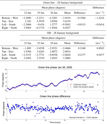
This self-consistency of ERWIN II is further demonstrated by considering the averages of these sectors for several days, shown in Table 1. Since the winds in opposing directions should have the same magnitude but opposite sign, the sum of these values should be zero. The table provides the val-ues of the average daily phase for each of the four sectors corresponding to the cardinal directions for three days in January 2009 for the hydroxyl and green-line observations. The means for each sector over the three days is calculated (4th column) and then the sum of the phases of opposite sectors determined. Since the winds in opposing directions should have the same magnitude, but opposite sign, the sum of these values should be close to zero, as observed. On av-erage, the difference is of the order of 1 m s−1. This further validates that the background is suitable for the wind deter-minations and at most a systematic error of 1 m s−1is intro-duced into the radial wind observations. The use of this phase background has been checked for the subsequent years and it is a stable feature of the interferometer.
Table 1. Comparisons of the mean differences of the daily averages of the opposite sight directions for the green-line and OH emissions using the 28 January 2009 background phase.
Green line – 28 January background
Mean phase (degrees) Difference
23 Jan 25 Jan 26 Jan Mean Difference (m s−1)
Bottom – West −2.2689 −5.2311 −4.3201 −3.9419 −0.3266 −1.4216
Top – East 2.183 5.5978 3.0596 3.6154
Left – South −2.3606 −0.424 1.2777 −0.5042 −0.0115 −0.0416 Right – North 3.5065 −0.1719 −1.8564 0.4927
OH – 28 January background
Mean phase (degrees) Difference
23 Jan 25 Jan 26 Jan Mean Difference (m s−1)
Bottom – West −1.885 −2.6528 −2.9221 −2.4866 0.1948 0.8563 Top – East 1.9366 3.4263 2.6872 2.6814
Left – South −2.5153 −2.7731 −0.8938 −2.0626 0.2177 0.9477 Right – North 3.4492 2.3319 1.0542 2.2804
Fig. 5. (a) Plot of green-line-emission zenith phase (blue dots) and the calibration phase (red dots) on 26 January 2009. The measurement uncertainty of the phase measurements is smaller than the size of the dots in this plot. (b) Plot of the difference between the zenith phase and the calibration phase interpolated using cubic splines to the times of the atmospheric observations. The zenith observations include geophysical variability. The time is UTC.
Depending on the thermal stability of the instrument short-term measurement errors can also be introduced if the ther-mal drift is not followed with sufficient precision. As de-scribed earlier, initially calibration phase measurements were taken on a slower cadence than the measurements. For the first two years of observations, one scan of the calibration lamps was taken for every eight scans of the atmospheric emissions. For the third year (March 2010 to March 2011) this was increased to a calibration every measurement scan of the atmospheric emissions.
Figure 5b (lower panel) is a time series of the difference between the observed zenith phase and the calibration phase interpolated using cubic splines to the times of the atmo-spheric observations. In this figure the measurement preci-sion is close to the size of the dots. The standard deviation of the difference is 1.02◦or 4.5 m s−1. This number includes geophysical variability (vertical winds, volume emission rate variations) and Schott noise and hence is not a clean mea-sure of the uncertainty introduced through the thermal-drift calibrations.
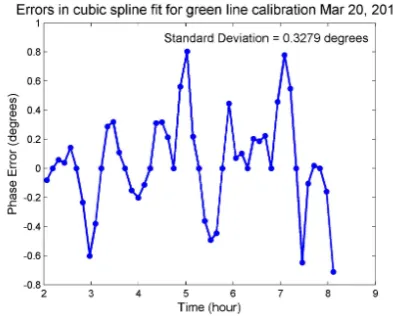
To explore this aspect of the measurement in more detail, an experiment which included frequent calibration measure-ments was performed (a calibration measurement was taken after every atmospheric measurement). The resulting calibra-tion phase time series was compared to one constructed by sampling this time series at a the same rate as other typical days and then interpolating (using cubic splines) these mea-surements to the times of the original time series. This pro-cess duplicated the thermal phase determinations associated with the atmospheric measurements
Figure 6 shows the result of this experiment. The phase error in the cubic spline is never more than a degree, and the standard deviation of the phase error over the duration of this experiment is 0.328◦(1.43 m s−1). This is significantly smaller than the standard deviation of the difference of the calibration phase and the zenith emission phase, which was 1.02◦(4.5 m s−1). This demonstrates that the errors associ-ated with the cubic spline are acceptably small compared to the other errors and geophysical noise. This uncertainty is reduced for observations with the more frequent calibration cadence.
Using the value of “a” appropriate for the 8-step scan, and substituting appropriately in Eqs. (2) and (4), the fol-lowing expression for the standard deviation (which we use as a measure of the wind precision) is obtained:
σw = c λ
4π 1effU V √
I. (14)
Hereσw is the error in m s−1,1eff is the effective path dif-ference,U V is the visibility, I is the observed number of photons detected per integration time per step in the absence of interference effects, cis the speed of light and λis the wavelength of the emission. The wind standard deviation is inversely proportional toU V, the path difference and the square root ofI. Comparison of the estimated variance using this formula to the observed variance provides an indication of how closely the observations conditions during individual scans match the assumptions associated with the derivation of this formula (namely that the source radiance and visibil-ity remain constant during a scan).
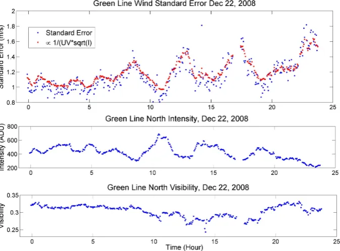
This is illustrated in Fig. 7, which provides time series of the actual standard error and the standard error estimated us-ing Eq. (12) (calculated as a variance for each bin in the sec-tor using Eq. (14) and then averaged in the same way as the
Fig. 6. Plot of the error in the cubic spline interpolation for the green-line calibration lamp sampled every∼30 min relative to the original time series and interpolated to the times of the original time series. Every 8th point of the original time series is used for the in-terpolation (the error for these points is identically zero).The data were recorded on 20 March 2010.
actual standard error is calculated), the signal (in analogue to digital units – ADU) and visibility for the north sector on 22 December 2008. The variability in both data sets is due to variations in the airglow volume emission rate (primar-ily) and visibility during that day. The expected decrease in the standard error when the signal increases (and vice versa) is evident in the upper two plots. It is striking that the two measures follow each other so closely since this indicates that intensity and visibility variations during individual scans are generally insignificant. If they are a factor then the stan-dard error would be significantly larger than the estimated precision.
Fig. 7. Comparison of the standard error (blue points) for northern sector compared to theσw(red points). Below this panel the corresponding detected signal (in ADU, middle panel) and visibility (lower panel) as a function of time for the same day are shown. Decreases in the standard error are mainly associated with increases in the signal as expected given the visibility stays roughly constant throughout the day.
Fig. 8. Standard errors for each of the cardinal direction sectors of the CCD on from 26 January 2009.
Plots of the winds provide a final, and satisfactory, check that the results are accurate. Meridional winds from 23 Jan-uary 2009 for green line and hydroxyl calculated in sev-eral different ways are shown in Fig. 9. The meridional, north direction and south direction winds are calculated us-ing Eqs. (5)–(7), respectively. The time series designated “without subtracting zenith” is a time series of the wind
determined from the northern sector without zenith sub-tracted. The meridional winds are reasonable, and indi-cate that there was a significant semi-diurnal tidal variation present. The manner in which this wind is determined renders it independent of vertical wind and thermal drift. Although perturbations due to gravity waves will result in small devi-ations from the true large-scale meridional wind above the station, to good approximation this time series can be con-sidered a good measure of the true meridional wind. Issues with thermal-drift, zero-wind or background phase will result in the meridional winds determined solely from the north or south directions deviating significantly from this time series. All the green-line winds agree well with each other. The north and south winds, which are the winds determined from the respective sectors with the zenith phase subtracted off to remove any thermal drift, follow the meridional wind very closely. This demonstrates that the winds viewed from the different directions are self-consistent. The fourth wind plotted on this figure is the north wind without the zenith phase subtracted. Since this also fits the meridional wind very closely, it demonstrates that the thermal drift has been effec-tively removed from the wind phase for observations with this emission.
Fig. 9. Time series of meridional winds (m s−1) from 23 January 2009 for the green-line (a) and hydroxyl emission (b) observations showing the consistency of the observations in the north and south directions when thermal drift and zero wind are appropriately accounted for and the problems – green points – in (b) when they are not. The standard errors of these observations are approximately the size of the points in the figure. Detailed discussion is in the text.
As expected, since there are no calibration measurements to provide thermal-drift information, omission of the zenith phase results in winds which exhibit significant systematic errors.
Since the contribution of the thermal-drift variance to the wind observations is ∼2.85 m2s−2 for the time when the longer cadence calibration period was implemented, it is pos-sible to use the zenith phase to examine the vertical wind (for the shorter cadence calibration period this will be even more feasible). While the exploration of this possibility will require careful analysis, an indication that this is plausible comes from a comparison (see Fig. 10) between the vertical wind determined using the zenith phase (blue dots) and the vertical wind determined using Eq. (10) (black dots). Both of these methods provide similar results on the larger tempo-ral scales. Over the day, the vertical wind is modulated sinu-soidally by a few m s−1. This could be due to a diurnal tide, although since this day was during the 2009 major strato-spheric warming, other dynamical effects could be present (Manney et al., 2009). The variance in the directly measured vertical wind is 30.9 m2s−2, which is significantly greater than the contribution associated with the thermal-drift deter-mination. The variance in the indirect determination of the vertical wind is 89.4 m2s−2. This calculation however also includes contributions from horizontal motions due to grav-ity waves and other high wave number phenomena. Further analysis of the vertical winds will be undertaken in the fu-ture to determine whether definitive geophysical results are possible.
In this section, the various factors affecting the precision and accuracy of the ERWIN II wind results have been dis-cussed and results demonstrating the internal consistency of the winds presented. The main factors affecting the mea-surement precision are the uncertainties associated with
Fig. 10. Green-line vertical wind (m s−1) 25 January 2009 as di-rectly observed (blue dots) and as calculated using the north, south, east and west winds (black dots) according to Eq. (10).
On these days the standard error will be less than 1 m s−1for observations during which the calibration cadence was high. The measurement accuracy for radial winds is determined by the uncertainty in the background phase determination (<1 m s−1) and uncertainties in the zero-wind determina-tion. Based on the arguments presented in Sect. 4, this is ex-pected to be less that 1 m s−1also. Hence, for the best obser-vation procedure (high cadence calibrations), the precision and accuracy are both∼1 m s−1.
6 Discussion
Comparisons between the capabilities of ERWIN II and other optical wind measuring instruments are not straightforward. Although theoretical comparisons based on throughput con-siderations have been undertaken (see Shepherd, 2002), few papers have discussed the precision and accuracy of a tech-nique in practice in as much detail and as clearly as has been undertaken in this paper. In part this is because a standard for comparison has not been developed, in part because the precision is dependent on the integration time (i.e. amount of light collected), instrument aperture and field of view, and thermal stability, and lastly in part because clear identifica-tion of the zero wind is difficult in practice. Instead, estimates of the measurement precision tend to be embedded in mea-surement papers using the particular technique in question. Since most techniques use some sort of average of the verti-cal wind over a night to estimate the true zero, unless there are other systematic errors, one can assume that the measure-ment accuracies are similar. As a result the measuremeasure-ment pre-cision (taken as the standard deviation of the velocity deter-mination) and the integration time needed for the measure-ment as quoted in the literature are the only pragmatic means to use in comparing different instruments.
For ERWIN II, five velocity measurements at a precision of 1 m s−1 in 45 s are observed for an airglow brightness slightly below average. In a recent paper on multiple order Fabry–Perot wind observations (Shiokawa et al., 2012) (sim-ilar to the observation technique used by Makela et al., 2011 and Meriwether et al., 2011) random errors ranging from 2 to 13 m s−1are quoted for a single wind observation with an ex-posure time of 60 s. Assuming that observing conditions in the middle of this range correspond to those for ERWIN II, it would take this instrument∼5 min to observe the same five velocities with a precision of∼7 m s−1.
The Scanning Doppler Interferometer (SCANDI) de-scribed by Arulia et al. (2010) is used for all-sky auroral imaging by using multiple fringes. They note that it takes ∼7–8 min to obtain a 25-sector wind measurement for these emissions, which are about an order of magnitude greater in brightness than they are at mid-latitudes (i.e. airglow as with ERWIN-II). For measurements on 8 March 2007 an uncertainty of 15 m s−1is quoted. Assuming that the mea-surement uncertainty scales roughly as the reciprocal of the
square root of the brightness, the uncertainty in these mea-surements would be∼45 m s−1(i.e. 15 m s−1×√10) for a brightness an order of magnitude less than that observed. If this was reduced to a 5-sector measurement by combining the observed irradiances, then the precision would be∼20 m s−1 (i.e. 45/√5) for a∼7 min measurement.
The DASH instrument (Englert et al., 2007) was recently used in field measurements at a mid-latitude site to compare results to a Fabry–Perot interferometer (Englert et al., 2012). For this comparison, 5 min integrations were taken and the oxygen red line was observed. Uncertainties at the one sigma level ranged from∼5 to 15 m s−1based on the plots in this paper. It would take>25 min to achieve the 5-measurement cycle of ERWIN II at a precision≥5 m s−1.
This comparison indicates that the precision and measure-ment cadence achieved by ERWIN II is significantly superior to any others reported in the literature. Of these, the multiple order Fabry–Perot of Shiokawa et al. (2012) comes closest to the ERWIN II performance. Even with this instrument (again assuming the uncertainty scales with number of photons de-tected per step as described above) it would require an inte-gration time of 225 min (5 min×72) to achieve the 1 m s−1 precision that ERWIN II achieves. These comparisons are not definitive since the instruments described in these papers do not necessarily represent their optimal configuration. How-ever, the advantage shown by ERWIN II is unlikely to be matched by minor changes in the configurations of these in-struments. At this time it provides the most precise and rapid airglow wind measurements in the world.
Rockets, lidar and radar are three other techniques used to measure winds in the mesopause region. Although compar-isons with the precision of the wind measurements associ-ated with these techniques are undertaken below, other im-portant aspects of the dynamical fields are measured using these instruments (for example temperature and density with lidar and diffusion with rockets and radar). In addition, their measurements may be more extensive that those undertaken with ERWIN II (i.e. inclusion of day/night observations or a greater height range and vertical resolution).
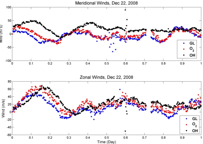
Fig. 11. Time series of the zonal and meridional winds for all three emissions on 22 December 2008. It is interesting to note that larger scale variations first show up in the green-line winds, followed by O2and then OH. This is expected for upward propagating tides for which the phase front propagates downward. Standard errors for each wind measurement are smaller than the dots in the figure for green line and OH and about the size of the dot for O2.
Frank et al. (2005) which compares lidar winds to meteor radar winds are quoted as being a few m s−1for (time/height) bins of (60 min/4 km). For the lidar used in this study, vec-tor winds were obtained with∼1 m s−1 precision between 85 and 100 km with a 12 min cycle and vertical resolution of ∼1 km (Liu and Gardener, 2005).
As discussed by Franke et al. (2005) and Fujii et al. (2004), the geometries of the observing conditions associated with the various wind measuring instruments are different. They are sensitive to different temporal and spatial scales, so the measurement variances are affected differently by geophysi-cal variability. ERWIN II views a brightness-weighted wind, so as noted in Sect. 3 it can be considered to provide winds for a volume of atmosphere of ∼5 km in the vertical and 5 km by 6 km in the horizontal In contrast, the lidar collects information from volumes with heights of 1 km and a diam-eter of∼50 m and the meteor radar collects information per velocity measurement from a volume 4 km thick and 200 km diameter (Franke et al., 2005). The sampling area of the MU radar per velocity measurement is from a volume 1 km thick and 200 km in diameter. Based on the height range and ver-tical resolution of the best of these various instruments, the lidar achieves 15 velocity measurements at a 1 m s−1 preci-sion in 12 min, and the MU radar achieves 40 velocity mea-surements at a 3–5 m s−1precision (recent upgrades to the MU radar may have enhanced its capabilities). With a vec-tor wind measurement every 45 s at a precision of∼1 m s−1, ERWIN II has similar capabilities to these instruments. For a
cycle through the three emissions, winds at nominal heights of 7, 93 and 97 km at the four cardinal directions and the vertical are obtained every three minutes at a precision equal to or better than these instruments and at a measurement ca-dence faster than either of these instruments. On the other hand, these instruments provide better spatial resolution than ERWIN II (especially in the vertical) since the observation volumes associated with each measurement are smaller.
Some indication of the capabilities of ERWIN II for sci-entific purposes is shown in Fig. 11. Here time series of the meridional and zonal winds observed by ERWIN II on 22 December 2008 for all three emissions are presented. As expected for larger scale upward propagating waves, the phase progression is downward with the green-line winds leading, followed by O2 and then OH. Standard errors for each wind measurement are smaller than the dots in the fig-ure for green line and OH and about the size of the dot for O2. The smaller scale variations are real and provide the op-portunity to investigate the wind fields at these heights on smaller temporal scales than previously possible. Given that ERWIN II simultaneously provides observations of the rela-tive brightness of the airglow emissions that it observes, the relationship between the winds and airglow can be explored in detail. Of particular interest is the investigation of grav-ity waves and the associated vertical velocities and airglow variations.
the upper mesosphere and lower thermosphere. These in-clude an All-Sky Imager (ASI) (observes OH, Na, O(1S), O(1D) and N+2), a spectral airglow temperature imager (SATI: O2, OH; Sargoytchev et al., 2004; Shepherd et al., 2010), and a meteor radar (Manson et al., 2009). The mea-surement cadences of the ASI and SATI are of the order of minutes, and the meteor radar provides an hourly vertical profile of horizontal wind in the mesopause region. Inter-comparisons between simultaneous observations taken with these instruments open up many possibilities for new sci-entific studies. Initial comparisons between ERWIN II and the meteor radar show them to be in reasonable agreement (a comparison which deals with the complexities of the ob-servational filters of each instrument will be published sep-arately). The dynamical signatures of specific events (such as stratospheric warming), wave signatures and the relation-ships between temperature, wind and emission rate over a broad range of scales are topics which this research station is especially capable of investigating.
7 Conclusions
The construction of ERWIN II and the completion of new data analysis algorithms have resulted in a powerful new ca-pability for investigating the dynamics of the mesopause re-gion. The most important physical changes to the instrument include the addition of a quad mirror to the ERWIN optical train so that multiple viewing directions can be simultane-ously observed and the inclusion of a CCD camera so that each of these directions can be simultaneously imaged. The new data analysis algorithm takes advantage of the imaging capabilities of the new instrument to provide a more pre-cise and better monitored wind and volume emission rate observations.
In this paper the capabilities of this instrument have been thoroughly discussed. For the standard observation se-quence, wind measurements have a precision and accuracy of∼1 m s−1and a 3 min observation cadence which incor-porates observations in five viewing directions for each of three different emissions. This accuracy, precision and ob-serving cadence was shown to be the best to date for optical instruments which use airglow to measure winds. Compar-isons with superior radar and lidar systems indicate that ER-WIN II wind observations are among the best in the world.
New science is anticipated with this instrument. On its own, vertical winds and relationships between the wind com-ponents and airglow volume emission rate can be investi-gated at temporal scales previously unachievable. Of partic-ular interest in this respect is the investigation of the relation-ships between these variables in gravity waves and tides, and the investigation of the velocity spectra at these heights.
The installation of ERWIN II at PEARL, along with sev-eral other instruments which observe temperature, airglow and wind in the mesopause region, establishes a unique
and potent capability both amongst Arctic observatories and worldwide. These instruments include a SATI, an All-Sky Imager and a meteor radar. Together they support the inves-tigation of the spatial and temporal variability of the tem-perature, wind and airglow on temporal scales of minutes to months and spatial scales from kilometres to hundreds of kilometres.
Acknowledgements. The Canadian Network for the Detection of Atmospheric Change (CANDAC)/PEARL funding partners are as follows: the Arctic Research Infrastructure Fund, Atlantic Innovation Fund/Nova Scotia Research Innovation Trust, Canadian Foundation for Climate and Atmospheric Science, Canadian Foundation for Innovation, Canadian Space Agency, Environment Canada, Government of Canada International Polar Year, Natural Sciences and Engineering Research Council, Ontario Innovation Trust, Ontario Research Fund, Indian and Northern Affairs Canada, and the Polar Continental Shelf Program. Funds from the Canadian Foundation of Innovation were essential for the construction of the ERWIN II instrument. Research support through grants from the Natural Sciences and Engineering Council (NSERC), research funding from the Canadian Foundation for Climate and Atmo-spheric Science (CFCAS), and support from the CREATE program of NSERC as well as the University of New Brunswick and York University are acknowledged. Financial support for Stephen Brown was provided through the CRESS Space Instrumentation Laboratory (CSIL) at York University. Brian Solheim and Gordon Shepherd are also thanked for their support of the design and construction of ERWIN II.
Edited by: A. Stoffelen
References
Anderson, C., Conde, M., and McHarg, M. G.: Neutral thermo-spheric dynamics observed with two scanning Doppler imagers: 1. Monostatic and bistatic winds, J. Geophys. Res., 117, A03304, doi:10.1029/2011JA017041, 2012.
Aruliah, A. L., Griffin, E. M., Yiu, H.-C. I., McWhirter, I., and Char-alambous, A.: SCANDI – an all-sky Doppler imager for studies of thermospheric spatial structure, Ann. Geophys., 28, 549–567, doi:10.5194/angeo-28-549-2010, 2010.
Bhattacharya, Y. and Gerrard, A. J.: Wintertime mesopause re-gion vertical winds from Resolute Bay, J. Geophys. Res., 115, D00N07, doi:10.1029/2010JD014113, 2010.
Chu, Y. H., Su, C. L., Larsen, M. F., and Chao, C. K.: First measurements of neutral wind and turbulence in the meso-sphere and lower thermomeso-sphere over Taiwan with a chem-ical release experiment, J. Geophys. Res., 112, A02301, doi:10.1029/2005JA011560, 2007.
Englert, C. R., Harlander, J. M., Brown, C. M., Meriwether, J. W., Makela, J. J., Castelaz, M., Emmert, J. T., Drob, D. P., and Marr, K. D.: Coincident thermospheric wind measurements using ground-based Doppler Asymmetric Spatial Heterodyne (DASH) and Fabry–Perot Interferometer (FPI) instruments, J. Atmos. Sol.-Terr. Phy., 86, 92–98, 2012.
Fisher, G. M., Killeen, T. L., Wu, Q., Reeves, J. M., Hays, P. B., Gault, W. A., Brown, S., and Shepherd, G. G.: Polar cap meso-sphere wind observations: Comparisons of simultaneous mea-surements with a Fabry–Perot interferometer and a field-widened Michelson interferometer, Appl. Optics, 39, 4284–4291, 2000. Fisher, G. M., Niciejewski, R. J., Killeen, T. L., Gault, W. A.,
Shep-herd, G. G., Brown, S., and Wu, Q.: Twelve-hour tides in the win-ter northern polar mesosphere and lower thermosphere, J. Geo-phys. Res., 107, 1211, doi:10.1029/2001JA000294, 2002. Franke, S. J., Chu, X., Liu, A. Z., and Hocking, W. K.: Comparison
of meteor radar and Na Doppler lidar measurements of winds in the mesopause region above Maui, Hawaii, J. Geophys. Res., 110, D09S02, doi:10.1029/2003JD004486, 2005.
Fujii, J., Nakamura, T., Tsuda, T., and Shiokawa, K.: Comparison of winds measured by MU radar and Fabry–Perot interferometer and effect of OI5577 airglow height variations, J. Atmos. Sol.-Terr. Phy., 66, 573–583, 2004.
Gault, W. A., Brown, S., Moise, A., Liang, D., Sellar, G., Shepherd, G. G., and Wimperis, J.: ERWIN: An E region wind interferom-eter, Appl. Optics, 35, 2913–2922, doi:10.1364/AO.35.002913, 1996.
Hilliard, R. L. and Shepherd, G. G.: Wide-Angle Michelson Inter-ferometer for measuring Doppler line widths, J. Opt. Soc. Am., 56, 362–369, 1966.
Kristoffersen, S. K.: The E-Region Wind Interferometer (ERWIN): Description of the Least Mean Squares Data Analysis Routine, Wind Results and Comparisons with the Meteor Radar, Univer-sity of New Brunswick, Fredericton, NB, Canada, 2012. Larsen, M. F.: Winds and shears in the mesosphere and
lower thermosphere: Results from four decades of chem-ical release wind measurements, J. Geophys. Res., 107, doi:10.1029/2001JA000218, 2002.
Liu, A. Z. and Gardner, C. S.: Vertical heat and constituent transport in the mesopause region by dissipating grav-ity waves at Maui, Hawaii (20.7◦N), and Starfire Optical Range, New Mexico (35◦N), J. Geophys. Res., 110, D09S13, doi:10.1029/2004JD004965, 2005.
Makela, J. J., Meriwether, J. W., Huang, Y., and Sherwood, P. J.: Simulation and analysis of a multi-order imaging Fabry–Perot interferometer for the study of thermospheric winds and temper-atures, Appl. Optics, 50, 4403–4416, 2011.
Manney, G. L., Schwartz, M. J., Kr¨uger, K., Santee, M. L., Paw-son, S., Lee, J. N., Daffer, W. H., Fuller, R. A., and Livesey, N. J.: Aura Microwave Limb Sounder observations of dy-namics and transport during the record-breaking 2009 Arctic stratospheric major warming, Geophys. Res. Lett., 36, L12815, doi:10.1029/2009GL038586, 2009.
Manson, A. H., Meek, C. E., Chshyolkova, T., Xu, X., Aso, T., Drummond, J. R., Hall, C. M., Hocking, W. K., Jacobi, Ch., Tsut-sumi, M., and Ward, W. E.: Arctic tidal characteristics at Eureka (80◦N, 86◦W) and Svalbard (78◦N, 16◦E) for 2006/07: sea-sonal and longitudinal variations, migrating and non-migrating tides, Ann. Geophys., 27, 1153–1173, doi:10.5194/angeo-27-1153-2009, 2009.
Meriwether, J. W., Makela, J. J., Huang, Y., Fisher, D. J., Bu-riti, R. A., Medeiros, A. F., and Takahashi, H.: Climatology of the nighttime equatorial thermospheric winds and temperatures over Brazil near solar minimum, J. Geophys. Res., 116, A04322, doi:10.1029/2011JA016477, 2011.
Press, W. H., Teukolsky, S. A., Vetterline, W. T., and Flannery, B. P.: Numerical Recipes The Art of Scientific Computing, 3rd Edn., Cambridge University Press, Cambridge, 2007.
Sargoytchev, S. I., Brown, S., Solheim, B. H., Cho, Y.-M., Shep-herd, G. G., and L´opez-Gonz´alez, M. J.: Spectral airglow tem-perature imager SATI: a ground-based instrument for the moni-toring of mesosphere temperature, Appl. Optics, 43, 5712–5721, 2004.
She, C. Y., Sherman, J., Yuan, T., Williams, B. P., Arnold, K., Kawa-hara, T. D., Li, T., Xu, L. F., Vance, J. D., Acott, P., and Krueger, D. A.: The first 80-hour continuous lidar campaign for simulta-neous observation of mesopause region temperature and wind, Geophys. Res. Lett., 30, 1319, doi:10.1029/2002GL016412, 2003.
Shepherd, G. G.: Spectral Imaging of the Atmosphere, Elsevier Academic Press, London, UK, 2002.
Shepherd, G. G., Thuillier, G., Gault, W. A., Solheim, B. H., Her-som, C., Alunni, J. M., Brun, J.-F., Charlot, P., Cogger, L. L., Desaulniers, D.-L., Evans, W. F. J., Gattingert, R. L., Girod, F., Harvie, D., Hum, R. H., Kendall, D. J. W., Llewellyn, E. J., Lowe, R. P., Ohrt, J., Pasternak, F., Peillet, O., Powell, I., Ro-chon, Y., Ward, W. E., Weins, R. H., and Wimperis, J.: WINDII, the wind imaging interferometer on the Upper Atmosphere Re-search Satellite, J. Geophys. Res., 98, 10725–10750, 1993. Shepherd, M. G., Cho, Y.-M., Shepherd, G. G., Ward, W.
E., and Drummond, J. R.: Mesospheric Temperature and Atomic Oxygen Response during the January 2009 Ma-jor Stratospheric Warming, J. Geophys. Res., 115, A07318, doi:10.1029/2009JA015172, 2010.
Shiokawa, K., Otsuka, Y., Oyama, S., Nozawa, S., Satoh, M., Katoh, Y., Hamaguchi, Y., and Yamamoto, Y.: Development of low-cost sky-scanning Fabry–Perot interferometers for air-glow and auroral studies, Earth Planets Space, 64, 1033–1046, doi:10.5047/eps.2012.05.004, 2012.
Ward, W. E.: Design and Implementation of a Wide Angle Michel-son Interferometer to Observe Thermospheric Winds, Ph.D. The-sis, York University, Toronto, Ont, Canada, 1988.