Is the Atlantic Multidecadal Oscillation (AMO) a statistical phantom?

(1)

Nonlin. Processes Geophys., 18, 469–475, 2011 www.nonlin-processes-geophys.net/18/469/2011/ doi:10.5194/npg-18-469-2011

Nonlinear Processes

in Geophysics

Is the Atlantic Multidecadal Oscillation (AMO) a statistical

phantom?

M. Vincze and I. M. J´anosi

Department of Physics of Complex Systems, Eötvös Loránd University, Pázmány P. s. 1/A, 1117 Budapest, Hungary Received: 10 January 2011 – Revised: 16 June 2011 – Accepted: 5 July 2011 – Published: 14 July 2011

Abstract. In this work we critically compare the conse-quences of two assumptions on the physical nature of the AMO index signal. First, we show that the widely used ap-proach based on red noise statistics cannot fully reproduce the empirical correlation properties of the record. Second, we consider a process of long range power-law correlations and demonstrate its better fit to the AMO signal. We show that in the latter case, the multidecadal oscillatory mode of the smoothed AMO index with an assigned period length of 50–70 years can be a simple statistical artifact, a conse-quence of limited record length. In this respect, a better term to describe the observed fluctuations of a smooth power-law spectrum is Atlantic Multidecadal Variability (AMV).

1 Introduction

The title of this work is adopted from a remarkable article by Godfrey et al. (2002), where the authors pointed out that mere sampling effects perfectly explain a famous weather folklore (January Thaw), which is an illusory regular warm deviation from the annual cycle during late January in the northeastern US. A more direct motivation of our analysis is provided by Thompson et al. (2010), who have reported on a rapid drop in Northern Hemisphere sea surface tempera-tures (SST) around 1970. The timescale of the observed drop is much shorter than changes in tropospheric aerosol load-ings or slow internal variability such as the Atlantic Multi-decadal Oscillation (AMO) index, challenging previous at-tempts to explain global patterns of 20th century climate variables. Thompson et al. (2010) argue that filtering out high frequency components from a signal can lead to infor-mation loss about existing physical processes of relatively

Correspondence to: I. M. J´anosi ([email protected])

short characteristic times, thus easily masking e.g. jumpwise changes. Fluctuations of mean SST on monthly timescales are usually considered as “pure noise” which has nothing to do with oceanic dynamics, therefore only “slow enough” (like AMO) modes are respected as physical signals.

There is a vast literature regarding the question whether a climatic time series is in fact a result of a pure de-terministic process with some characteristic frequency or a stochastic process which exhibits “apparent” periodic-ity (see e.g. Knight, 2009, and references therein). Best known examples are probably the North-Atlantic Oscilla-tions (NAO) (Hurrell, 1995), the Southern Oscillation In-dex (SOI) (Trenberth, 1984; Cane and Zebiak, 1985), the Dansgaard–Oeschger events (Ditlevsen et al., 2005) or the glacial-interglacial oscillations that most theories have tried to link to the Milankovitch forcing while others suggested underlying stochastic mechanisms (Ganopolski and Rahm-storf, 2002; Ashkenazy and Tziperman, 2004; Huybers and Wunsch, 2005).

Low frequency oscillations of cool and warm phases in sea surface temperatures in the North Atlantic basin have been identified in instrumental data since 1856 (Kushnir, 1994; Schlesinger and Ramankutty, 1994; Sutton and Allen, 1997; Kerr, 2000; Enfield et al., 2001; Goldenberg et al., 2001) and in proxy data for centuries (Gray et al., 2004). The term At-lantic Multidecadal Oscillation (AMO) was coined by Kerr (2000). The AMO index is introduced by Enfield et al. (2001) as a ten years running mean of monthly SST anoma-lies, averaged over the Atlantic basin, north of the Equator. The smoothed time series (shown in Fig. 1) exhibits cooler than average SST values in the periods 1900–1925 and 1965– 1995 with warmer periods at the end of the nineteenth cen-tury, during 1925–1965, and in the last decade. Note that a global linear trend is removed from the original monthly time series, however it is so weak (the mean SST warming slope is 2.16×10−3K yr−1) that it makes no difference in the fol-lowing analysis. The relative shortness of the instrumental

(2)

470 M. Vincze and I. M. J´anosi: Is AMO a statistical phantom? Manuscript prepared for Nonlin. Processes Geophys.

with version 3.2 of the LA_{TEX class copernicus.cls.} Date: 11 July 2011

Is the Atlantic Multidecadal Oscillation (AMO) a statistical

phantom?

Mikl´os Vincze and Imre M. J´anosi

Department of Physics of Complex Systems, Eötvös Loránd University, Pázmány P. s. 1/A, H-1117 Budapest, Hungary

Abstract. In this work we critically compare the conse-quences of two assumptions on the physical nature of the AMO index signal. First, we show that the widely used ap-proach based on red noise statistics cannot fully reproduce the empirical correlation properties of the record. Second, we consider a process of long range power-law correlations and demonstrate its better fit to the AMO signal. We show that in the latter case, the multidecadal oscillatory mode of the smoothed AMO index with an assigned period length of 50-70 years can be a simple statistical artifact, a consequence of limited record length. In this respect, a better term to de-scribe the observed fluctuations of a smooth power-law spec-trum is Atlantic Multidecadal Variability (AMV).

1 Introduction

The title of this work is adopted from a remarkable article by Godfrey et al. (2002), where the authors pointed out that mere sampling effects perfectly explain a famous weather folklore (January Thaw), which is an illusory regular warm deviation from the annual cycle during late January in the northeastern U.S. A more direct motivation of our analysis is provided by Thompson et al. (2010), who have reported on a rapid drop in Northern Hemisphere sea surface temper-atures (SST) around 1970. The timescale of the observed drop is much shorter than changes in tropospheric aerosol loadings or slow internal variability such as the Atlantic Mul-tidecadal Oscillation (AMO) index, challenging previous at-tempts to explain global patterns of 20th century climate variables. Thompson et al. (2010) argue that filtering out high frequency components from a signal can lead to infor-mation loss about existing physical processes of relatively short characteristic times, thus easily masking e.g., jumpwise Correspondence to: I. M. J´anosi

([email protected])

1900 1950 2000

year -2

-1 0 1 2

standardized AMO index

Fig. 1. Standardised monthly mean SST anomalies (thin line) and AMO index (ten years running mean, thick line and red/blue colours) calculated from the Kaplan SST data set which is updated monthly at http://www.cdc.noaa.gov/Timeseries/AMO/.

changes. Fluctuations of mean SST on monthly timescales are usually considered as “pure noise” which has nothing to do with oceanic dynamics, therefore only “slow enough” (like AMO) modes are respected as physical signals.

There is a vast literature regarding the question whether a climatic time series is in fact a result of a pure de-terministic process with some characteristic frequency or a stochastic process which exhibits “apparent” periodic-ity (see e.g., Knight (2009) and references therein). Best known examples are probably the North-Atlantic Oscilla-tions (NAO) (Hurrell, 1995), the Southern Oscillation In-dex (SOI) (Trenberth, 1984; Cane and Zebiak, 1985), the Dansgaard–Oeschger events (Ditlevsen et al., 2005) or the glacial-interglacial oscillations that most theories have tried to link to the Milankovitch forcing while others suggested underlying stochastic mechanisms (Ganopolski and Rahm-Fig. 1. Standardised monthly mean SST anomalies (thin line) and AMO index (ten years running mean, thick line and red/blue colours) calculated from the Kaplan SST data set which is updated monthly at http://www.cdc.noaa.gov/Timeseries/AMO/.

climate record compared to an assumed period length of 50– 70 years, however, limits confidence of clearly establishing a real oscillatory mode.

This impression is further strengthened by comparing the instrumental signal with the tree ring proxy record by Gray et al. (2004) in Fig. 2. The reconstructed annual mean SST anomaly, and its ten years running mean (proxy AMO) have a somewhat limited overlap with the instrumental signals in the appropriate time interval, nevertheless the proxy AMO lacks the signature of a more or less stable oscillatory mode. An alternative definition of AMO index was proposed by Trenberth and Shea (2006). The main difference is that they computed mean SST values for the world ocean and de-termined the difference between this “background” and the North-Atlantic average. This modified AMO index has a de-creased variability, however the “warm” and “cold” phases are almost overlap with the signal shown in Fig. 1. Other modifications, effects of different detrending and background removal procedures and problems with the signal interpreta-tions are summarized in details by Knight (2009).

Numerical models have a distinguished role to simulate much longer periods than covered by reliable measurements (Frankignoul and Hasselmann, 1977; Delworth et al., 1993; Timmermann et al., 1998; Dong and Sutton, 2005; Jungclaus et al., 2005; Knight et al., 2005; Frankcombe et al., 2009; Knight, 2009; Ottera et al., 2010). The key element com-mon in all models is a link between the AMO and the At-lantic meridional overturning circulation, however character-istic time scales of the variability are not satisfactorily ex-plained. A recent numerical work by Park and Latif (2010) has produced an AMO signal over a simulated interval of 1000 years, and multidecadal oscillations of a characteris-tic period about 60 years have identified. Note, however,

that this result is obtained by band-pass filtering of the orig-inal SST time series in the period range 30–90 years, and the authors have consistently used the term Atlantic Multi-decadal Variability (AMV) instead of AMO throughout the paper (Park and Latif, 2010). The picture is further com-plicated by observations of variability on 20–30 year time scales of sub-surface temperature (Frankcombe et al., 2008), and tide gauge records (Frankcombe and Dijkstra, 2009) in the North Atlantic.

Here we propose that the mean SST anomaly signals ex-hibit long range power-law correlations, instead of being a simple low-order autoregressive process. (Long range cor-relations for local SST values are detected already by e.g. Monetti et al. (2003).) As a consequence, the apparent multi-decadal oscillation represented by the AMO index can be ex-plained as a simple finite size effect. We do not question the variability of mean SST anomalies on timescales of decades, however we intend to refine the picture by demonstrating the probable lack of a fixed characteristic frequency. This finding can resolve the many controversial estimates on oscillatory time scales in simulations and proxy reconstructions.

2 Correlation properties

In order to compare measured and artificial model time se-riesx(t ), we always perform the usual standardisation by the empirical mean value hxi and standard deviation σ =

p

hx2_{i − h}_x_i2 _as_{X(t )}_{= [}_{x(t )}_{− h}_x_i]_/σ_{, as in Figs. 1 and 2.} We will return to the importance of this step at the particular tests.

Since the partial autocorrelation function of the standard-ised monthly mean SST anomalyIn(Fig. 1) drops to zero in a single step (not shown here), moving average (MA) pro-cesses cannot come into question (von Storch and Zwiers, 1999). Fits of autoregressive AR(m) models with increasing orders mdo not results in a significant improvement com-pared to the simplest first order AR(1) hypothesis:

In+1=a1In+ξn , (1)

wherea1=0.9034684, and ξn is a random variable drawn from a Gaussian IID ensemble of standard deviation σξ= σI

q

1−a₁2=0.428654 (note thatσI≡1 as a consequence of standardisation). As a measure of goodness of fit, we list the square-root mean error (based on observed value minus one-step-ahead forecast) for AR(m) fits withm=1...5: 0.4310, 0.4311, 0.4306, 0.4301, 0.4294. Even atm=20, the mean forecast error remains 0.4247, the improvement is negligible. As a next step, we produced an artificial series of 185 500 data points by iterating Eq. (1) with the fitted parameters, and split into 100 pieces of equal length of the original monthly mean SST anomaly series. The scatter plot of the empirical mean value and standard deviation for each individual piece is shown in Fig. 3 with black circles. As expected, the split-ting resulted in some statistical shifts at the short segments,

(3)

M. Vincze and I. M. J´anosi: Is AMO a statistical phantom? 471

2 M. Vincze and I. M. J´anosi: Is AMO a statistical phantom?

1600 1650 1700 1750 1800 1850 1900 1950 2000

year

-2 -1 0 1 2 3 4 5 6

standardized AMO index

Enfield et al. (2001)

Gray et al. (2004)

Fig. 2. Top: standardized annual mean SST anomaly and AMO series as in Fig. 1, shifted upward for a clear visualisation. Bottom:

Standardised annual mean SST anomaly (thin line) and its ten years running mean (thick line, red and blue coloured) determined from the tree ring proxy data set by Gray et al. (2004) ftp://ftp.ncdc.noaa.gov/pub/data/paleo/.

storf, 2002; Ashkenazy and Tziperman, 2004; Huybers and Wunsch, 2005).

Low frequency oscillations of cool and warm phases in sea surface temperatures in the North Atlantic basin have been identified in instrumental data since 1856 (Kushnir, 1994; Schlesinger and Ramankutty, 1994; Sutton and Allen, 1997; Kerr, 2000; Enfield et al., 2001; Goldenberg et al., 2001) and in proxy data for centuries (Gray et al., 2004). The term At-lantic Multidecadal Oscillation (AMO) was coined by Kerr (2000). The AMO index is introduced by Enfield et al. (2001) as a ten years running mean of monthly SST anoma-lies, averaged over the Atlantic basin, north of the Equator. The smoothed time series (shown in Fig. 1) exhibits cooler than average SST values in the periods 1900–1925 and 1965– 1995 with warmer periods at the end of the nineteenth cen-tury, during 1925–1965, and in the last decade. Note that a global linear trend is removed from the original monthly time series, however it is so weak (the mean SST warming slope is2.16×10−3_{K/year) that it makes no difference in the}

fol-lowing analysis. The relative shortness of the instrumental climate record compared to an assumed period length of 50-70 years, however, limits confidence of clearly establishing a real oscillatory mode.

This impression is further strengthened by comparing the instrumental signal with the tree ring proxy record by ? in Fig. 2. The reconstructed annual mean SST anomaly, and its ten years running mean (proxy AMO) have a somewhat lim-ited overlap with the instrumental signals in the appropriate time interval, nevertheless the proxy AMO lacks the signa-ture of a more or less stable oscillatory mode.

An alternative definition of AMO index was proposed by ?. The main difference is that they computed mean SST

values for the world ocean and determined the difference between this “background” and the North-Atlantic average. This modified AMO index has a decreased variability, how-ever the “warm” and “cold” phases are almost overlap with the signal shown in Fig. 1. Other modifications, effects of different detrending and background removal procedures and problems with the signal interpretations are summarized in details by Knight (2009).

Numerical models have a distinguished role to simulate much longer periods than covered by reliable measurements (Frankignoul, and Hasselmann, 1977; Delworth et al., 1993; Timmermann et al., 1998; Dong, and Sutton, 2005; Jung-claus et al., 2005; Knight et al., 2005; Frankcombe et al., 2009; Knight, 2009; Ottera et al., 2010). The key element common in all models is a link between the AMO and the Atlantic meridional overturning circulation, however charac-teristic time scales of the variability are not satisfactorily ex-plained. A recent numerical work by Park and Latif (2010) has produced an AMO signal over a simulated interval of 1000 years, and multidecadal oscillations of a characteris-tic period about 60 years have identified. Note, however, that this result is obtained by band-pass filtering of the orig-inal SST time series in the period range 30–90 years, and the authors have consistently used the term Atlantic Multi-decadal Variability (AMV) instead of AMO throughout the paper (Park and Latif, 2010). The picture is further com-plicated by observations of variability on 20–30 year time scales of sub-surface temperature (Frankcombe et al., 2008), and tide gauge records (Frankcombe and Dijkstra, 2009) in the North Atlantic.

Here we propose that the mean SST anomaly signals ex-hibit long range power-law correlations, instead of being a Fig. 2. Top: standardised annual mean SST anomaly and AMO series as in Fig. 1, shifted upward for a clear visualisation. Bottom: standardised annual mean SST anomaly (thin line) and its ten years running mean (thick line, red and blue coloured) determined from the tree ring proxy data set by Gray et al. (2004) ftp://ftp.ncdc.noaa.gov/pub/data/paleo/.

simple low-order autoregressive process. (Long range cor-relations for local SST values are detected already by e.g., Monetti et al. (2003).) As a consequence, the apparent mul-tidecadal oscillation represented by the AMO index can be explained as a simple finite size effect. We do not ques-tion the variability of mean SST anomalies on timescales of decades, however we intend to refine the picture by demon-strating the probable lack of a fixed characteristic frequency. This finding can resolve the many controversial estimates on oscillatory time scales in simulations and proxy reconstruc-tions.

2 Correlation Properties

In order to compare measured and artificial model time se-ries x(t), we always perform the usual standardisation by the empirical mean value hxi and standard deviationσ= p

hx2_{i − h}_x_i2_as_X₍_t_{) = [}_x₍_t₎_{− h}_x_i_]_/σ_{, as in Figs. 1 and 2.} We will return to the importance of this step at the particular tests.

Since the partial autocorrelation function of the standard-ised monthly mean SST anomalyIn (Fig. 1) drops to zero

in a single step (not shown here), moving average (MA) pro-cesses cannot come into question (von Storch and Zwiers, 1999). Fits of autoregressive AR(m) models with increasing orders mdo not results in a significant improvement com-pared to the simplest first order AR(1) hypothesis:

In+1=a1In+ξn , (1)

where a1= 0.9034684, andξn is a random variable drawn

from a Gaussian IUD ensemble of standard deviationσξ=

σI

p 1−a2

1= 0.428654(note thatσI≡1as a consequence of

standardisation). As a measure of goodness of fit, we list the square-root mean error (based on observed value minus one-step-ahead forecast) for AR(m) fits withm= 1...5: 0.4310, 0.4311, 0.4306, 0.4301, 0.4294. Even atm= 20, the mean forecast error remains 0.4247, the improvement is negligible. As a next step, we produced an artificial series of 185500 data points by iterating Eq. (1) with the fitted parameters, and split into 100 pieces of equal length of the original monthly mean SST anomaly series. The scatter plot of the empirical mean value and standard deviation for each individual piece is shown in Fig. 3 with black circles. As expected, the split-ting resulted in some statistical shifts at the short segments, therefore standardisation was performed separately with the individual mean values and standard deviations prior to sub-sequent analysis.

Temporal correlation properties were evaluated by two methods: detrended fluctuation analysis (DFA) and Fourier transform (power spectrum). Both of them are considered nowadays as standard procedures, therefore we skip tech-nical details (“Google Scholar” gives almost four thousand hits for searching DFA). Here we emphasise only the key

as--3

-2

-1

0

1 mean value

0.6

0.8

1

1.2 standard deviation

AR(1)

lrc

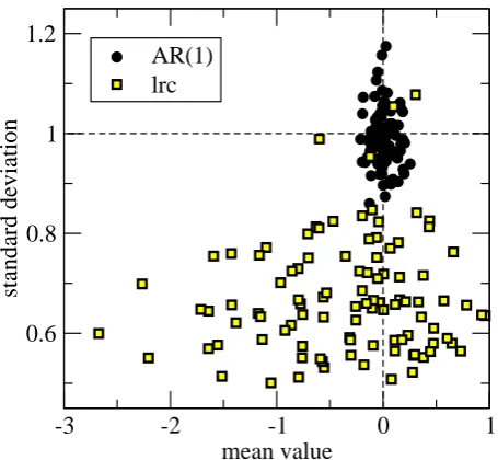
Fig. 3. Scatter plot of the individual mean values and standard devi-ations for two sets of model time series. The first series is produced by the AR(1) model Eq. (1) with the parameters fitted to the monthly SST signal. The second long-range correlated (lrc) signal of spec-tral exponentβ= 0.6is produced with the inverse Fourier method, see e.g. Fox (1987). Both time series of 185500 data points are split into 100 equal pieces, and the individual means and standard deviations are plotted (see legends).

with the computation of autocorrelation function) provide the very same information about two-point temporal corre-lations. For example, a long range correlated (lrc) process by definition obeys a power-law decaying autocorrelation function A(τ) =hX(t+τ)X(t)i ∼τ−α _{with an exponent}

0< α <1. Simultaneously, its power spectrum has a

simi-lar formS(f)∼f−β_{, and the DFA}p_{fluctuation function is}

also power-law: Fp(w)∼wδ. Furthermore, the exponents

obey cross-relations (Heneghan and McDarby, 2000), e.g.:

α= 2(1−δ) , β= 2δ−1 , α+β= 1 . (2)

The mathematical equivalence does not mean that these methods are equally efficient for finite (and often noisy) data, e.g. the Fourier transformation usually provides more robust result than a direct computation of the autocorrelation func-tion. The DFApprocedure has a benefit that it removes a global trend [a polynomial of order(p−1)] from the original series, thus it can handle nonstationarities.

For the very reason, we determined DFAp fluctuation functions withp= 2...5for the standardised monthly SST anomaly shown in Fig. 1 and for each AR(1) model sequence separately. Since we did not observe differences for increas-ingpvalues, we show only the results of DFA2 computations in Fig. 4a. For increasing time window sizesw(in units of month), the statistical inaccuracies result in a widening band for the model sequences, nevertheless their behaviour fol-Fig. 3. Scatter plot of the individual mean values and standard devi-ations for two sets of model time series. The first series is produced by the AR(1) model Eq. (1) with the parameters fitted to the monthly SST signal. The second long-range correlated (lrc) signal of spec-tral exponentβ=0.6 is produced with the inverse Fourier method, see e.g. Fox (1987). Both time series of 185500 data points are split into 100 equal pieces, and the individual means and standard deviations are plotted (see legends).

therefore standardisation was performed separately with the individual mean values and standard deviations prior to sub-sequent analysis.

Temporal correlation properties were evaluated by two methods: detrended fluctuation analysis (DFA) and Fourier transform (power spectrum). Both of them are considered nowadays as standard procedures, therefore we skip tech-nical details (“Google Scholar” gives almost four thousand hits for searching DFA). Here we emphasise only the key as-pect that in the mathematical sense these methods (together with the computation of autocorrelation function) provide the very same information about two-point temporal cor-relations. For example, a long range correlated (lrc) pro-cess by definition obeys a power-law decaying autocorrela-tion funcautocorrela-tionA(τ )= hX(t+τ )X(t )i ∼τ−αwith an exponent 0< α <1. Simultaneously, its power spectrum has a similar formS(f )∼f−β, and the DFApfluctuation function is also power-law: Fp(w)∼wδ. Furthermore, the exponents obey cross-relations (Heneghan and McDarby, 2000), e.g.: α=2(1−δ) , β=2δ−1 , α+β=1 . (2) The mathematical equivalence does not mean that these methods are equally efficient for finite (and often noisy) data, e.g. the Fourier transformation usually provides more robust result than a direct computation of the autocorrelation func-tion. The DFAp procedure has a benefit that it removes a global trend [a polynomial of order(p−1)] from the origi-nal series, thus it can handle nonstationarities.

For the very reason, we determined DFAp fluctuation functions withp=2...5 for the standardised monthly SST anomaly shown in Fig. 1 and for each AR(1) model sequence separately. Since we did not observe differences for increas-ingpvalues, we show only the results of DFA2 computations in Fig. 4a. For increasing time window sizesw(in units of month), the statistical inaccuracies result in a widening band for the model sequences, nevertheless their behaviour fol-lows the expectations (Kir´aly and J´anosi, 2002). For short

(4)

-1 -0.5 0 0.5 1 1.5 2

log

10

[F(w)]

1 1.5 2 2.5 3 3.5

log

₁₀

(w)

-1

-0.5 0 0.5 1 1.5 2

log

10

[F(w)]

(a)

(b)

½

Fig. 4. The logarithm of DFA2 fluctuations log10[F (w)]as a func-tion of the logarithm of sliding window size log10(w)for the model sequences (thin coloured lines) and for the monthly mean SST anomaly (thick black curve). The thick red line is the same for the tree ring proxy annual mean SST (see Fig. 2), also shown as a blue dashed line shifted upward. (a) Fitted AR(1) model series, and (b) long range correlated series withβ=0.6.

times an AR(1) process has strong “memory” indicated by a large slope of DFA curves, but this slope gradually decreases to the asymptotic value of 1/2. The empirical monthly SST sequence does not really fit into this band: the AR(1) model systematically overestimates observed correlations for the in-termediate times[40−135]months, and definitely underesti-mates them over 690 months (note the log10scales in Fig. 4). The limited length of the monthly SST anomaly series (1855 data points in our analysis) and observational noise un-avoidably yield to statistical uncertainties, nevertheless the black DFA curve in Fig. 4a seems to be much more lin-ear than the cyan AR(1) model curves. Therefore it seems plausible to test the assumption of long range power-law cor-relations (which would result in a straight line in Fig. 4a). Power-law correlated model series can be easily produced e.g. by the classical inverse-Fourier method, where the input

-1 -0.5 0 0.5 1 1.5 2

log

10

[F(w)]

1 1.5 2 2.5 3 3.5

log

₁₀

(w)

-1

-0.5 0 0.5 1 1.5 2

log

10

[F(w)]

(a)

(b)

½

Fig. 4. The logarithm of DFA2 fluctuations log10[F(w)]as a func-tion of the logarithm of sliding window size log10(w)for the model sequences (thin coloured lines) and for the monthly mean SST anomaly (thick black curve). The thick red line is the same for the tree ring proxy annual mean SST (see Fig. 2), also shown as a blue dashed line shifted upward. (a) Fitted AR(1) model series, and (b) long range correlated series withβ= 0.6.

times an AR(1) process has strong “memory” indicated by a large slope of DFA curves, but this slope gradually decreases to the asymptotic value of 1/2. The empirical monthly SST sequence does not really fit into this band: the AR(1) model systematically overestimates observed correlations for the in-termediate times[40−135]months, and definitely underesti-mates them over 690 months (note the log10scales in Fig. 4). The limited length of the monthly SST anomaly series (1855 data points in our analysis) and observational noise un-avoidably yield to statistical uncertainties, nevertheless the black DFA curve in Fig. 4a seems to be much more linear than the cyan AR(1) model curves. Therefore it seems plau-sible to test the assumption of long range power-law correla-tions (which would result in a straight line in Fig. 4a). Power-law correlated model series can be easily produced e.g. by the classical inverse-Fourier method, where the input is a

pre-10-3 10-2 10-1

0.001 0.01 0.1

frequency [1/month]

10-3

10-2 10-1

Fourier amplitudes

(a)

(b)

Fig. 5. Power spectra of (a) fitted AR(1) and (b) lrc model series (β= 0.6) (thin coloured lines), together with the spectrum for the monthly mean SST anomaly record (thick black line). Note the double-logarithmic scales. (In each case, the standard Welch win-dowing was applied prior to the Fourier transform.

scribed spectrum with a givenβand random phases, and the output is a scalar time series (Fox, 1987). (Some care should be taken to handle continuation upto the zero frequency, but the appropriate methods are also widely discussed in the lit-eraure.) The main difference between a long range correlated (lrc) and AR(1) series is clearly illustrated in Fig. 3 (yellow squares): the individual means and standard deviations cover a much larger range when a long standardised lrc sequence is split into shorter segments. In this case, the individual stan-dardisation is much more important to minimise statistical bias during subsequent tests.

Fig. 4b illustrates the DFA2 band for 100 individually standardised lrc model series of spectral exponent β= 0.6

(thin orange lines). Clearly, the black empirical curve fits much better into this band.

The thick red lines in Fig. 4 indicate the DFA2 curve for the tree ring proxy SST series (see Fig. 2). It covers a much longer time interval than the instrumental SST data (424 years in our analysis), however its temporal resolution of 1 Fig. 5. Power spectra of (a) fitted AR(1) and (b) lrc model series (β=0.6) (thin coloured lines), together with the spectrum for the monthly mean SST anomaly record (thick black line). Note the double-logarithmic scales. (In each case, the standard Welch win-dowing was applied prior to the Fourier transform.

is a prescribed spectrum with a givenβand random phases, and the output is a scalar time series (Fox, 1987). (Some care should be taken to handle continuation upto the zero frequency, but the appropriate methods are also widely dis-cussed in the literature.) The main difference between a long range correlated (lrc) and AR(1) series is clearly illustrated in Fig. 3 (yellow squares): the individual means and dard deviations cover a much larger range when a long stan-dardised lrc sequence is split into shorter segments. In this case, the individual standardisation is much more important to minimise statistical bias during subsequent tests.

Figure 4b illustrates the DFA2 band for 100 individually standardised lrc model series of spectral exponent β=0.6 (thin orange lines). Clearly, the black empirical curve fits much better into this band.

The thick red lines in Fig. 4 indicate the DFA2 curve for the tree ring proxy SST series (see Fig. 2). It covers a much longer time interval than the instrumental SST data (424

(5)

1 10 100

period [year] 10-6 10-5 10-4 10-3 10-2 10-1 Fourier amplitude monthly SST 10 years running mean

Fig. 6. Power spectra of the original monthly SST series (brown) and its 121 month running average, the AMO index (black with symbols), as a function of period length.

year limits the statistical confidence of a similar modeling procedure presented for the monthly record. Therefore we performed the fitting-model ling-splitting test only for the in-strumental monthly mean SST data. The DFA2 fluctuation function obviously has a lower magnitude for annual mean values compared to monthly fluctuations, and it is shifted on the horizontal axis as well. Still it is fully consistent with the DFA2 curve of the monthly SST series illustrated by the blue dashed lines in Fig. 4. It has the same slope, and enhances the difference between an lrc and an AR(1) process with an asymptotic DFA slope of 1/2 (see Fig. 4a).

As it is already mentioned, Fourier spectra convey the same mathematical information as DFApcorrelation curves (Ghil et al., 2002), nevertheless Fig. 5 further illustrates the differences between the basic model assumptions. Various versions of Fig. 5a appeared in many papers with the conclu-sion that the small frequency peak at around 0.0012-0.0017 month−1_{(according to a period of 50-70 years) is a}

statisti-cally significant signature of a clean oscillatory mode. How-ever, Fig. 5b demonstrates that the peak is not significant for an lrc process, it is rather a finite size effect. (The power spectrum for the annual proxy SST series is not shown, it sinks into the plotted bands.)

3 The effects of smoothing

Thompson et al. (2010) convincingly pointed out that an un-desirable side effect of high frequency filtering is the smear-ing out of jumpwise, abrupt changes, also in cases when the reason is some physical effect instead of noise. The defini-tion of AMO index contains the filtering by a 10-year running

-2 -1 0 1 2

0 240 480 720 960 1200 1440 1680

month

-2 -1 0 1 2

standardized AMO + models

(a)

(b)

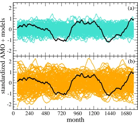
Fig. 7. Smoothed (121-point running mean) curves for (a) fitted AR(1), and (b) lrc model segments (thin coloured lines) after stan-dardisation. The heavy black curve is the same for the standardised monthly AMO series (also shown in Fig. 1).

mean (see Figs. 1 and 2) which certainly helps to distinguish “warm” and “cold” intervals.

Figure 6 illustrates the effects of the 121-point running mean smoothing of the original monthly SST series. The interesting fact is that all spectral components of period<

30 years are gradually suppressed, the highest frequencies are damped by more than two orders of magnitude. Mean-while, the low frequency tail remains intact. Unfortunately this means only 3-4 points in the Fourier space as a conse-quence of limited record length. Note that the spectrum of AMO index (black curve in 6) retains its continuous power-law shape, the presence of pronounced isolated peaks is not salient.

Our final test aims to check the effect of smoothing by the running mean filter of the two model sets, the results are shown in Fig. 7. Note again that 121-point running means were determined on individually standardised model seg-ments. The comparison of the cyan band in Fig. 7a with the AMO index suggests that the latter presents an extreme case if it is an AR(1) process, local minima and maxima coin-cide with the very edge of the model ensemble. However, when we assume that the AMO signal is an lrc process, the clean oscillation of a fixed frequency becomes an artifact of limited length and strong smoothing: Fig. 7b exhibits sev-eral model signals in the background (thin orange lines) with much larger amplitudes and similar length of “period”.

4 Conclusions

If we reject the hypothesis that the AMO signal represents a physical oscillatory mode of oceanic circulation, we should Fig. 6. Power spectra of the original monthly SST series (brown)

and its 121 month running average, the AMO index (black with symbols), as a function of period length.

years in our analysis), however its temporal resolution of 1 year limits the statistical confidence of a similar modeling procedure presented for the monthly record. Therefore we performed the fitting-modelling-splitting test only for the in-strumental monthly mean SST data. The DFA2 fluctuation function obviously has a lower magnitude for annual mean values compared to monthly fluctuations, and it is shifted on the horizontal axis as well. Still it is fully consistent with the DFA2 curve of the monthly SST series illustrated by the blue dashed lines in Fig. 4. It has the same slope, and enhances the difference between an lrc and an AR(1) process with an asymptotic DFA slope of 1/2 (see Fig. 4a).

As it is already mentioned, Fourier spectra convey the same mathematical information as DFApcorrelation curves (Ghil et al., 2002), nevertheless Fig. 5 further illustrates the differences between the basic model assumptions. Various versions of Fig. 5a appeared in many papers with the con-clusion that the small frequency peak at around 0.0012– 0.0017 month−1(according to a period of 50–70 years) is a statistically significant signature of a clean oscillatory mode. However, Fig. 5b demonstrates that the peak is not significant for an lrc process, it is rather a finite size effect. (The power spectrum for the annual proxy SST series is not shown, it sinks into the plotted bands.)

1 10 100

period [year] 10-6 10-5 10-4 10-3 10-2 10-1 Fourier amplitude monthly SST 10 years running mean

Fig. 6. Power spectra of the original monthly SST series (brown) and its 121 month running average, the AMO index (black with symbols), as a function of period length.

year limits the statistical confidence of a similar modeling procedure presented for the monthly record. Therefore we performed the fitting-model ling-splitting test only for the in-strumental monthly mean SST data. The DFA2 fluctuation function obviously has a lower magnitude for annual mean values compared to monthly fluctuations, and it is shifted on the horizontal axis as well. Still it is fully consistent with the DFA2 curve of the monthly SST series illustrated by the blue dashed lines in Fig. 4. It has the same slope, and enhances the difference between an lrc and an AR(1) process with an asymptotic DFA slope of 1/2 (see Fig. 4a).

As it is already mentioned, Fourier spectra convey the same mathematical information as DFApcorrelation curves (Ghil et al., 2002), nevertheless Fig. 5 further illustrates the differences between the basic model assumptions. Various versions of Fig. 5a appeared in many papers with the conclu-sion that the small frequency peak at around 0.0012-0.0017 month−1_{(according to a period of 50-70 years) is a}

statisti-cally significant signature of a clean oscillatory mode. How-ever, Fig. 5b demonstrates that the peak is not significant for an lrc process, it is rather a finite size effect. (The power spectrum for the annual proxy SST series is not shown, it sinks into the plotted bands.)

-2 -1 0 1 2

0 240 480 720 960 1200 1440 1680

month

-2 -1 0 1 2

standardized AMO + models

(a)

(b)

Fig. 7. Smoothed (121-point running mean) curves for (a) fitted AR(1), and (b) lrc model segments (thin coloured lines) after stan-dardisation. The heavy black curve is the same for the standardised monthly AMO series (also shown in Fig. 1).

Figure 6 illustrates the effects of the 121-point running mean smoothing of the original monthly SST series. The interesting fact is that all spectral components of period<

30 years are gradually suppressed, the highest frequencies are damped by more than two orders of magnitude. Mean-while, the low frequency tail remains intact. Unfortunately this means only 3-4 points in the Fourier space as a conse-quence of limited record length. Note that the spectrum of AMO index (black curve in 6) retains its continuous power-law shape, the presence of pronounced isolated peaks is not salient.

4 Conclusions

If we reject the hypothesis that the AMO signal represents a physical oscillatory mode of oceanic circulation, we should Fig. 7. Smoothed (121-point running mean) curves for (a) fitted AR(1), and (b) lrc model segments (thin coloured lines) after stan-dardisation. The heavy black curve is the same for the standardised monthly AMO series (also shown in Fig. 1).

Figure 6 illustrates the effects of the 121-point running mean smoothing of the original monthly SST series. The interesting fact is that all spectral components of period<30 years are gradually suppressed, the highest frequencies are damped by more than two orders of magnitude. Meanwhile, the low frequency tail remains intact. Unfortunately this means only 3–4 points in the Fourier space as a consequence of limited record length. Note that the spectrum of AMO index (black curve in Fig. 6) retains its continuous power-law shape, the presence of pronounced isolated peaks is not salient.

(6)

4 Conclusions

If we reject the hypothesis that the AMO signal represents a physical oscillatory mode of oceanic circulation, we should certainly comment on the opposite conclusions of the litera-ture. First of all, note that the appearance of the same or very similar AMO-like patterns in other climate variables mea-sured or reconstructed for the same 15–20 decades (Kushnir, 1994; Enfield et al., 2001; Goldenberg et al., 2001; Knight et al., 2006; Trenberth and Shea, 2006; Frankcombe et al., 2008; Thompson et al., 2010; Wang and Dong, 2010) does not prove the existence of a real oscillatory mode. It is widely accepted that large scale oceanic circulations are determining factors of the weather and climate, thus whatever changes SST over a significant geographic area, its effects will be ap-preciable in the whole coupled system.

The most popular explanation of the appearance of well defined oscillations in a noisy systems is based on mode selection. Indeed, model analysis by te Raa and Dijkstra (2002) and especially by Frankcombe et al. (2009) demon-strated that large scale oceanic circulation driven by differ-ential heating and rotation produces SST oscillations. Ac-cording to the results, both spatial and temporal correla-tions in the external noise were important for the excitation of possible multidecadal modes, with the amplitude of os-cillation increasing with stronger temporal correlation. Note however that statistical significance of the filtered time se-ries was tested by the red noise hypothesis (based on plots like Fig. 5a), thus the possible consequences of long range power-law correlations were not considered.

We repeat again, there is no doubt that low frequency SST variability is a prevailing feature of oceanic dynamics. Both DFA and Fourier spectral analysis suggest that the dominant time scales are indeed span over decades, because they have the strongest spectral magnitude. However both DFA and Fourier spectra exhibit a continuous power-law shape with-out the apparent presence of one (or more) well defined os-cillation frequency. As we have demonstrated, filtering has a side effect of giving enhanced weights of low frequency components, and limited record lengths can easily lead to the impression of strict periodicity.

Acknowledgements. This work was supported by the Hungarian

Science Foundation (OTKA) under Grant No. NK72037, the European Commissions RECONCILE-226365-FP7-ENV-2008-1 project, and by the European Union and the European Social Fund under the grant agreement no. T ´AMOP 4.2.1./B-09/1/KMR-2010-0003.

Edited by: W. Hsieh

Reviewed by: three anonymous referees

References

Ashkenazy, Y. and Tziperman, E.: Are the 41 kyr glacial oscilla-tions a linear response to Milankovitch forcing?, Quat. Sci. Rev., 23, 1879–1890, doi:10.1016/j.quascirev.2004.04.008, 2004. Cane, M. A. and Zebiak, S. E.: A theory for el nino and the southern

oscillation, Science, 228, 1085–1087, 1985.

Delworth, T. L., Manabe, S., and Stouffer, R. J.: Interdecadal variations of the thermohaline circulation in a coupled ocean-atmosphere model, J. Climate, 6, 1993–2011, 1993.

Ditlevsen, P. D., Kristensen, M. S., and Andersen, K. K.: The recurrence time of Dansgaard–Oeschger events and limits on the possible periodic component, J. Climate, 18, 2594–2603, doi:10.1175/JCLI3437.1, 2005.

Dong, B. and Sutton, R. T.: Mechanism of interdecadal thermoha-line circulation variability in a coupled ocean-atmosphere GCM, J. Climate, 18, 1117–1135, 2005.

Enfield, D. B., Mestas-Nu˜nez, A. M., and Trimble, P. J.: The At-lantic Multidecadal Oscillation and its relation to rainfall and river flows in the continental U.S., Geophys. Res. Lett., 28, 2077–2080, doi:10.1029/2000GL012745, 2001.

Fox, C. G.: An inverse Fourier transform algorithm for generating random signals of a specified spectral form, Computers Geosci., 13, 369–374, doi:10.1016/0098-3004(87)90009-4, 1987. Frankcombe, L. M. and Dijkstra, H. A.: Coherent multidecadal

variability in North Atlantic sea level, Geophys. Res. Lett., 36, L15604, doi:10.1029/2009GL039455, 2009.

Frankcombe, L. M., Dijkstra, H. A., and von der Heydt, A.: Sub-surface signatures of the Atlantic Multidecadal Oscillation, Geo-phys. Res. Lett., 35, L19602, doi:10.1029/2008GL034989, 2008. Frankcombe, L. M., Dijkstra, H. A., and von der Heydt, A.: Noise induced multidecadal variability in the North Atlantic: Excita-tion of normal modes, J. Phys. Oceanogr., 39, 220–233, 2009. Frankignoul, C. and Hasselmann, K.: Stochastic climate

mod-els, Part II, Application to sea-surface temperature anomalies and thermocline variability, Tellus, 29, 289, doi:10.1111/j.2153-3490.1977.tb00740.x, 1977.

Ganopolski, A. and Rahmstorf, S.: Abrupt glacial climate changes due to stochastic resonance, Phys. Rev. Lett., 88, 038501, doi:10.1103/PhysRevLett.88.038501, 2002.

Ghil, M., Allen, M. R., Dettinger, M. D., Ide, K., Kondrashov, D., Mann, M. E., Robertson, A. W., Saunders, A., Tian, Y., Varadi, F., and Yiou, P.: Advanced spectral methods for climatic time series, Rev. Geophys., 40, 1, doi:10.1029/2000RG000092, 2002. Godfrey, C. M., Wilks, D. S., and Schultz, D. M.: Is the January Thaw a statistical phantom?, B. Am. Meteorol. Soc., 83, 53–62, doi:10.1175/1520-0477(2002)083<0053:ITJTAS>2.3.CO;2, 2002.

Goldenberg, S. B., Landsea, C. W., Mestas-Nu˜nez, A. M., and Gray, W. M.: The recent increase in Atlantic hurricane activity: Causes and implications, Science, 293, 474–479. doi:10.1126/science.1060040, 2001.

Gray, S. T., Graumlich, L. J., Betancourt, J. L., and Pederson, G. T.: A tree-ring based reconstruction of the Atlantic Multidecadal Oscillation since 1567 A.D., Geophys. Res. Lett., 31, L12205. doi:10.1029/2004GL019932, 2004.

Heneghan, C. and McDarby, G.: Establishing the relation be-tween detrended fluctuation analysis and power spectral density analysis for stochastic processes, Phys. Rev. E, 62, 6103–6110, doi:10.1103/PhysRevE.62.6103, 2000.

(7)

Hurrell, J. W.: Decadal trends in the North Atlantic Oscillation: Regional temperatures and precipitation, Science, 269, 676–679, 1995.

Huybers, P. and Wunsch, C.: Obliquity pacing of the late Pleistocene glacial terminations, Nature, 434, 491–494, doi:10.1038/nature03401, 2005.

Jungclaus, J. H., Haak, H., Latif, M., and Mikolajewicz, U.: Arctic-North Atlantic interactions and multidecadal variability of the meridional overturning circulation, J. Climate, 18, 4013–4031, 2005.

Kerr, R. A.: A North Atlantic climate pacemaker for the centuries, Science, 288, 1984–1986, doi:10.1126/science.288.5473.1984, 2000.

Kir´aly, A. and J´anosi, I. M.: Stochastic modeling of daily temperature fluctuations, Phys. Rev. E, 65, 051102, doi:10.1103/PhysRevE.65.051102, 2002.

Knight, J. R.: The Atlantic Multidecadal Oscillation inferred from the forced climate response in coupled general circulation mod-els, J. Climate, 22, 1610–1625, doi:10.1175/2008JCLI2628.1, 2009.

Knight, J. R., Allan, R. J., Folland, C. K., Vellinga, M., and Mann, M. E.: A signature of persistent natural thermohaline circula-tion cycles in observed climate, Geophys. Res. Lett., 32, L20708, doi:10.1029/2005GL024233, 2005.

Knight, J. R., Folland, C. K., and Scaife, A. A.: Climate impacts of the Atlantic Multidecadal Oscillation, Geophys. Res. Lett., 33, L17706, doi:10.1029/2006GL026242, 2006.

Kushnir, Y.: Interdecadal variations in North Atlantic sea surface temperature and associated atmospheric conditions, J. Climate, 7, 141–157, 1994.

Monetti, R. A., Havlin, S., and Bunde, A.: Long-term persistence in the sea surface temperature fluctuations, Physica A, 320, 581– 589, doi:10.1016/S0378-4371(02)01662-X, 2003.

Ottera, O. H., Bentsen, M., Drange, H., and Suo, L.: External forc-ing as a metronome for Atlantic multidecadal variability, Nat. Geosci., 3, 688–694, doi:10.1038/NGEO955, 2010.

Park, W. and Latif, M.: Pacific and Atlantic multidecadal variabil-ity in the Kiel Climate Model, Geophys. Res. Lett., 37, L24702, doi:10.1029/2010GL045560, 2010.

Schlesinger, M. E. and Ramankutty, N.: An oscillation in the global climate system of period 65–70 years, Nature, 367, 723–726, doi:10.1038/367723a0, 1994.

Sutton, R. T. and Allen, M. R.: Decadal predictability of North Atlantic sea surface temperature and climate, Nature, 388, 563– 567, doi:10.1038/41523, 1997.

te Raa, L. A. and Dijkstra, H. A.: Instability of the thermohaline ocean circulation on interdecadal timescales, J. Phys. Oceanogr., 32, 138–160, 2002.

Thompson, D. W. J., Wallace, J. M., Kennedy, J. J., and Jones, P. D.: An abrupt drop in Northern Hemisphere sea surface temperature around 1970, Nature, 467, 444–447, doi:10.1038/nature09394, 2010.

Timmermann, A., Latif, M., Voss, R., and Grotzner, A.: Northern Hemisphere interdecadal variability: A coupled air-sea mode, J. Climate, 11, 1906–1931, 1998.

Trenberth, K. E.: Signal versus Noise in the Southern Oscillation, Mon. Weather Rev., 112, 326–332, 1984.

Trenberth, K. E. and Shea, D. J.: Atlantic hurricanes and nat-ural variability in 2005, Geophys. Res. Lett., 33, L12704, doi:10.1029/2006GL026894, 2006.

von Storch, H. and Zwiers, F. W.: Statistical Analysis in Climate Research, Cambridge Univ. Press, Cambridge, 1999.

Wang, C. and Dong, S.: Is the basin-wide warming in the North Atlantic Ocean related to atmospheric carbon diox-ide and global warming?,, Geophys. Res. Lett., 37, L08707, doi:10.1029/2010GL042743, 2010.