www.nonlin-processes-geophys.net/17/85/2010/ © Author(s) 2010. This work is distributed under the Creative Commons Attribution 3.0 License.
Nonlinear Processes
in Geophysics
Variable predictability in deterministic dissipative sandpile
M. G. Shnirman1,3and A. B. Shapoval2,3
1Institut de Physique du Globe de Paris, UMR 7154, CNRS, France
2Finance Academy under the Government of the Russian Federation, Russia
3International Institute of Earthquake Prediction Theory and Mathematical Geophysics, Russia
Received: 24 February 2009 – Revised: 19 January 2010 – Accepted: 11 February 2010 – Published: 24 February 2010
Abstract. It is known that some quiescence precedes the strong events in the Bak–Tang–Wiesenfeld sand-pile (Pepke and Carlson, 1994). We introduce dissipation depending on the propagation of the events into this model such that in the constructed model the growth of activity occurs before the strong events. This fact allows the prediction of them in ad-vance with a certain efficiency. This efficiency is variable in time. The best predictability is observed during subcritical time ranges, while the efficiency is definitely worse in the supercritical state.
1 Introduction
The attitude to earthquake prediction remains controversial (Wyss, 1997). On the one hand, there exist the prediction al-gorithms which efficiently forecast strong earthquakes in ad-vance (Kossobokov and Shebalin, 2003). The foreshock ac-tivity of middle-size earthquakes underlies these algorithms (Keilis-Borok, 2003). On the other hand, some scientists ar-gue that these algorithms hardly reflect the physics of the seismicity and that the efficiency of the current outcome of the prediction will decline later (Geller et al., 1997).
This discussion is based on the comprehension of the seis-mic process as a movement of a self-organized critical sys-tem of blocks. A typical example of a self-organized critical system is the sandpile introduced by Bak, Tang, and Wiesen-feld (BTW) in Bak et al. (1987). Their model determines the evolution of sand grains on a lattice. The grains are slowly accumulated until their number becomes locally too big. Then they are instantaneously redistributed over the lat-tice. The redistribution mechanism is conservative inside the lattice and dissipative at the boundary. The slow input and
Correspondence to: A. B. Shapoval ([email protected])
the quick output balance each other and the system comes to its steady state (Dhar, 1999). Model reviews and open prob-lems can be found at Dhar (2006); Dickman et al. (2000).
According to Pepke and Carlson (1994), (a) strong model events have the anti-activation scenario; (b) the adapted earthquake precursors predict these events with a very low efficiency. Further investigation (Shapoval and Shnirman, 2004) of the BTW sandpile gives evidence that its biggest events (which rarely happen) are predictable due to precur-sors that are unobservable in seismicity. The irregularity of the dissipation (examined by De Menech et al., 1998) and the oscillation of the sand-pile height underlie the prediction. In details, when the number of the grains in the lattice is small the system stays in its subcritical state characterized by a weak dissipation and a rare occurrence of the middle-size events. Then the lattice accumulates “extra” grains and the system comes to the supercritical state. It returns to the subcritical state when a characteristic event happens (De Menech et al., 1998). Just the latter event is predictable due to the quiescence preceding it (Shapoval and Shnirman, 2004). Still, the absence of activation prior to strong events contradicts either the critical self-organization of the seismic process or the predictability of earthquakes based on a cer-tain activation. The “wrong” scenario of strong model events probably happens due to the conservative redistribution of the grains inside the lattice, whereas the fault interactions are dissipative.
rule such that dissipation of the full-scale events is unpropor-tionally bigger than dissipation of the small events.
This dissipation leads to the activation scenario of strong events. The constructed model remains predictable but the growth of activity underlies the prediction of strong events. The prediction algorithm corresponds to that for real seismic-ity (Keilis-Borok, 2003). The highest efficiency of prediction is attained when the system comes to the subcritical state.
2 Model 2.1 Dynamics Let{(i,j )}L
i,j=1be a square lattice. The set of the integers 4= {hij}Li,j=1is called a “configuration”. These integers are interpreted as the heights of the sand grains on the cell(i,j ). The cell(i,j ) is stable ifhij< H, where H=4 is the
cell instability threshold. Ifhij>H, then the cell(i,j )is
unstable. Further, the configuration4is called “stable” if all its cells are stable. Otherwise, the configuration is unstable.
Let a random variable take the values 0, 1, 2, 3 with the probability of 1/4. Then itsL2independent observations de-termine the initial configuration40. Evidently,40is stable.
Now we define the mechanism transforming the configu-ration4(t )appearing at the time stept to4(t+1). Initially, the mechanism adds a new grain onto the central cell(i0,j0): hi0j0−→hi0j0+1.
If the cell(i0,j0)remains stable nothing more occurs at this time stept. Then the configuration4(t+1)is obtained. If hi0j0>4 then sand is redistributed.
We start the definition of the redistribution with one act initiated by any unstable cell(i,j ). Let hij>4. Then the
unstable cell passes four grains one-by-one to its four nearest neighbours. Several grains can dissipate during this pass:
hij −→hij−4−Dij, (1)
hc(i,j )−→hc(i,j )+1 ∀c(i,j ), (2)
wherec(i,j )is any cell such that it has a common side with (i,j )andDij is some non-negative integer. ThenDij grains
dissipate if the cell(i,j )does not belong to the lattice bound-ary. The redistribution on the boundary results in one (or two for the corners) additional dissipated grain since the bound-ary cells have less than four neighbours. It worth reminding thatDij=0 in the BTW sand-pile.
Clearly, the act of the redistribution can lead to the for-mation of new unstable cells. The redistribution starts in the central cell(i0,j0)and continues until a stable configuration occurs (during the redistribution one cell can become unsta-ble several times). The final configuration is just4(t+1). Then the next time step begins.
Two time scales are defined in the model. The grain ad-dition occurs during slow time (the word “slow” is usually omitted). The redistribution is associated with quick time.
2.2 Dissipation
It remains to defineDij. Letzij be the counters of the cell
instability. It is supposed thatzij=0∀i,j at the beginning
of any time step. Once the cell(i,j )becomes unstable the counterzij increases by one. The threshold valuez∗is fixed
for all the counterszij. By definition, put
Dij=
0, if zij< z∗;
d∗, if zij>z∗,
(3) where d∗ is some natural number. Thus in addition to a boundary dissipation we define an internal dissipation de-pending on the redistribution of the grains.
Our model depends on two parameters: z∗andd∗. The valuez∗determines when the dissipation is switched on. The valued∗stays for the number of the dissipating grains during one act of the redistribution.
The value of the instability thresholdHdoes not influence the model dynamics. We fixH=4 to make easier the com-parison with the BTW sand-pile. In this case the heights can become negative due to dissipation. However they are still bounded from below. Whence, movingH higher makes all the heights positive. Interpretinghij as the local stress we
keep in mind the model with sufficiently bigH.
If the redistribution occurs at some time step then this pro-cess is called an event. Its size is the number of the unstable cells appeared during the redistribution and counted with re-gard for multiplicity.
The model differs from the BTW sand-pile in two ways. First, new grains are added not in cells chosen at random but in the lattice center only (as discussed in Wiesenfeld et al., 1990). This makes the dynamics deterministic. Secondly, the dissipationDij differs from zero.
3 Power recurrence law
The BTW sand-pile has gained popularity due to its power recurrence law. We draw the corresponding plot for the con-structed model. Let a catalogue be the set of the consequent events. The catalogue has to be sufficiently extent and remote from the initial configuration such that the system is able to attain the steady state. Suppose1sis some fixed number be-ing insignificantly bigger than one. LetF (s)be the number of the catalogued events, whose size lies inσ∈ [s/1s,s1s), divided by the extent of the catalogue (in other words, by the number of the grains added). IfF (s)is a power function then its graph is linear in the log-log scale.
101 102 103 104 10−3
10−2
s F
−0.15
−0.12
z*=4,d*=1 z*=5,d*=1 z*=10,d*=1 z*=20,d*=1 z*=infinity z*=10,d*=10
Fig. 1. The frequencyF (s)vs. the sizesfor the different models;
“z∗=infinity” stays for the BTW model with a central seeding; the slopes of the dashed lines are−0.12 and−0.15; the catalogues’ extent is 5×10⁵;L=128;1s=100.1.
values of the parameterz∗mean that the dissipationDij is
(almost always) equal to zero (according to Eq. 3). Then the model dynamics agrees with the BTW sand-pile with grain addition in the central cell. Ifz∗ is small the dissipation is switched on so early that the strong events are hardly real-ized. Therefore the graph forz∗=4,d∗=1 lies significantly lower than the others.
Note that the function F (s) exhibits locally cumulative size distribution. This increases the slope of the power part of the graphs by 1 (in the log-log scale) comparatively with the direct size-frequency plot given, for example in Wiesenfeld et al. (1990) for the BTW model with the central seeding.
4 Prediction
4.1 Precursor “Power Size” (PSi)
There are prediction algorithms forecasting strong earth-quakes in advance (Keilis-Borok and Kossobokov, 1990; Keilis-Borok and Rotwain, 1990; Kossobokov and Shebalin, 2003; Shebalin, 2006). The precursors of the strong earth-quakes underlying these algorithms quantitatively describe the increase of the middle-size earthquakes prior to the strong earthquakes. We are going to adapt these precursors to the big model events. The event is called “target” if its size is bigger than some s0. The target events correspond to the strong earthquakes. Suppose[s−,s+],s−< s+< s0, is the size interval of the middle-scale events,wis the length of the
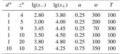
Table 1. Optimal values of the parameters fixed for different pairs
(d∗,z∗).
d∗ z∗ lg(s−) lg(s+) α w T
1 4 2.80 3.80 0.25 300 100 1 5 3.00 4.00 0.25 200 100 1 9 3.45 4.45 0.25 70 300 1 10 3.50 4.50 0.25 100 100 1 20 3.80 4.80 0.25 100 300 10 10 3.25 4.25 0.75 350 100
sliding window, ands(t )∈ [s−,s+]is the size of the middle-scale event occurred at the time stept. Then the functional
9α(t )= t−1 X k=t−w
s(k)α, (4)
whereαis an appropriate power, is a precursor (of the target events) measuring the occurrence of the middle-scale events. We name this precursor “Power Size” (PSi) as well as the prediction algorithm based on this precursor. Prediction al-gorithm PSi includes the calculation of the precursor and a rule switching alarms on and off. As soon as 9α(t ) > 9∗
(for appropriate fixed 9∗) the algorithm expects a target event to occur during the nextT time steps. More precisely, let ton be any time step specified by 9α(ton) > 9∗. Then toff=ton+T is assigned totonif the target events are absent on[ton,ton+T]. Otherwise bytoffdenote the step of the first target events. Then the union of all[ton,toff](which possibly intersect one another) forms a time of increased probability (TIP) of the target events. The target events are said to be predicted if they occur during TIP.
4.2 Prediction efficiency
The ratio of the unpredicted events and the TIP extent natu-rally describe the prediction efficiency (Keilis-Borok, 2003; Molchan, 2003). Supposen is the ratio of the unpredicted events,τis the ratio of TIP (in other words,τ is the total TIP extent divided by the catalogue length), andεisn+τ. Then εis called the loss of the algorithm. According to Molchan (2003), the lossεis close to 1 for a random prediction. The efficiency of the prediction is 1−ε.
4.3 Choice of parameters
4 8 12 16 0.5
0.6 0.7 0.8 0.9
3.9
4.1
4.55
4.6
4.9
z* ε
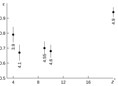
Fig. 2. The lossεwith error bars vs. the thresholdz∗switching
the dissipation on ford∗=1. The numbers are the values of log(s0) (the lowest size of the target events).
The low boundarys0of the target events is not adjusted. Aiming at the best efficiency we chooses0as big as possible (this idea works for the BTW sand-pile; Shapoval and Shnir-man, 2004). The fixed values ofs0(being written in Fig. 2 forL=128) ensure approximately the same frequency of the target events in the catalogues for differentz∗. Despite these values of s0 are bigger than the sizes shown in Fig. 1 the number of the target events in the catalogue is big enough to get statistically significant results.
4.4 Prediction outcome
Figure 2 introduces the loss εfor the prediction algorithm corresponding to the dissipationd∗=1 and several values of z∗. Ifz∗is too big algorithm PSi does not predict the target events. This agrees with the BTW sand-pile. Small values of z∗(z∗=4 in Fig. 2) lead to a weak predictability. The strong events are extremely rare in such models.
The best predictability is observed for intermediate z∗ (Fig. 2). These values ofεare far from 1. This gives evidence that the prediction results are not random. Moreover, the ef-ficiency increases whenever the dissipation goes up. We do not support this statement for allz∗but give the detailed anal-ysis of the predictability in the model determined byz∗=10, d∗=10.
So, fixz∗=10,d∗=10. Algorithm PSi is applied to the catalogue sampled during[2.5×106,7.5×106] time steps (L=128; 5×10⁶grains are added on the lattice). It keeps 2601 target events. The algorithm predicts 2185 events while the alarm continues about a third of the catalogue’s extent. In other words, the outcome of the prediction isn=0.16,τ=
0.35,ε=0.51. To check this result other catalogues of the same length are generated for different initial configurations. The values ofε=n+τ≈0.5 are conserved.
The parameters of the algorithm PSi influence the effi-ciency in a different way. The most principal parameters are wandT. On the contrary, the parameterαdetermining the power in the functional9α defined in Eq. (4) weakly
influ-ences the efficiency. We claim that the loss of the algorithm PSi is less than 0.54 asα∈ [0.1,1].
4.5 Role of dissipation
We have determined the nonlinear dissipation depending on the propagation of the model events. This dissipation weak-ens the middle-scale events preventing their propagation. Therefore it takes the series of the middle-scale events to transport the grains to the boundary. Only then the full-scale event happens. Hence it can be predicted. This scheme gives the explanation of the reported prediction efficiency. 4.6 Efficiency variability
By definition, put
h(t )=L−2
L X i,j=1
hij(t ),
where the values ofhij(t )are taken at the end of the time
stept. Further, supposehhi(t )is the mean ofh(t )over previ-ousNs=50 000 time steps andhεi(t )is the lossεcalculated
on[t−Ns,t]. Then the oscillations ofhεi(t )are rather big
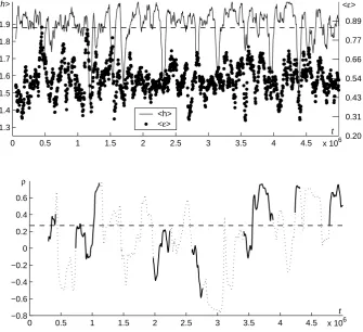
(Fig. 3). The loss can be doubled (from 0.35 to 0.70) due to the choice of the prediction interval. Is this variability con-nected with the sandpile height, which changes significantly too (Fig. 3)?
By ρ(t ) we denote the correlation function of hεi(t ) and hhi(t ). It is calculated on the intervals [t−Nb,t],
Nb=250 000. NumbersNs andNbbalance two opposite
re-quirements. On the one hand, the used intervals have to be small such that the model properties described in terms of h(t )do not change a lot. On the other hand, if the intervals are too small then their number of the target event remains insufficient for meaningful conclusions about the prediction efficiency.
According to Fig. 3, lower panel, there exist extremely long time ranges (hundreds of thousand time steps) exhibit-ing the correlationρof the constant sign. Still the mean of the correlation function is close to zero.
4.7 Sub- and supercriticality
0 0.5 1 1.5 2 2.5 3 3.5 4 4.5 1.3
1.4 1.5 1.6 1.7 1.8 1.9
t <h>
x 1060.20
0.31 0.43 0.54 0.66 0.77 0.89 <ε>
<h>
<ε>
0 0.5 1 1.5 2 2.5 3 3.5 4 4.5
−0.8 −0.6 −0.4 −0.2 0 0.2 0.4 0.6
t ρ
x 106
Fig. 3. A typical evolution of the smoothed height’s mean, prediction efficiency (upper panel), and their correlation functionρ(t )(lower
panel) ford∗=10,z∗=10;hhi(t )andhεi(t )are the the average ofh(t )and, respectively, the loss of the prediction, over[t−5×10⁴,t ). The dotted curve stays forρ(t )on the cutting off intervals with too low sand level. The solid curves stay for the other intervals. The mean of the solid curves (ofhhi(t )) is approximately 0.27 (1.88, dashed lines). Zero on the time axes corresponds to the beginning of the catalogue.
We want to analyze only the parts of the correlation func-tion in which the average height is greater than or equal to an arbitrary threshold,hhi(t ) < h∗, because a part of our hy-pothesis is that better prediction is not possible when the av-erage height is low (corresponding to few events). Conse-quently, for each time stept0 wherehhi(t0) < h∗, we iden-tify the corresponding time interval (in the past) over which
hhi(t0)was previously defined, namely[t0−Ns,t0]. We want
to exclude all the points that lie in this interval from the cal-culation of any future values of the correlation functionρ(t ). First, notice that time steps within this “forbidden” interval will be used in the calculation ofhhi(t )for all values oft in
[t0,t0+Ns]. Second, notice that time steps within the interval [t0,t0+Ns+Nb]will determineρ(t )using values ofhhi(t )
which themselves use data from the “forbidden” interval. Therefore, for any value oft0for whichhhi(t0) < h∗, we mark the interval[t0,t0+Ns+Nb]with a dotted line in the
correla-tion plot of Fig. 3 to signify regions with poor predictability due to low system average height (or low system mass). The remaining part of the correlation plot is marked with thick solid line to identify regions with better predictability.
According to Fig. 3, the remaining part ofρ(t ) (plotted by the solid line) is more positive than negative. The mean
¯
ρ of this ρ(t )-part shown in the figure is 0.27 (for reliable conclusion the mean is calculated for two other catalogues; the values are 0.25 and 0.30). Hence the height and the ef-ficiency fluctuate co-directionally if the height is close to its critical level. Then the growth of the height usually increases the lossε of the prediction algorithm. If the height is near its critical level then the height’s growth pushes the system to the supercritical state. Thus the co-directional oscillations of hεi(t )andhhi(t )give an implicit evidence that the pre-dictability is worse in the supercritical state.
The value ofh∗has to be sufficiently big to study the sys-tem near its critical level of height. However excessively bigh∗s eliminate the graph of ρ(t )completely. It is fixed h∗=1.7 whenever the mean ofh(t )is approximately 1.88. (We check the values ofh∗for three considered catalogues; h∗=1.65 implies ρ¯=0.14;0.25;0.30 and h∗=1.75 does
¯
ρ=0.26;0.27;0.21; this calculation gives evidence of a cer-tain stability of the results with respect toh∗).
calculation corresponds to Fig. 3’s all the intervals such that h(t )belongs to[1.7,1.85]and[1.92,2.0]during at least 500 consequent time steps.
The following idea can explain the observed variability. If the number of the grains on the lattice is too big then even minor changes in the configurations are able to generate a strong event. A long formation process is not necessary. A strong event can occur “at any moment”. Therefore the pre-dictability is weaker in the supercritical state. Furthermore, extremely low pile height assures that the growth of activity in a lattice part does not lead to a strong event because the other part lacks the sand grains. A strong event would occur later (and remain unpredictable) when the lattice accumu-lates some additional grains and a new wave of the redistri-bution attains the overloaded lattice part. This leads to a low prediction efficiency. Finally, whenever the height comes to its critical level from below there exists the formation process of the strong events involving the increase of activity. 4.8 Accuracy of results
The properties of the prediction developed in the paper can be sensitive to the choice of the parameters. The applied scheme searches the minimum ofεthrough a limited num-ber of points lying in the many-dimensional parameter space. On the one hand, the lossεof the prediction as the function in any particular parameter has aV-shape on the grid if the values of the other parameters are fixed as reported in Table 1 (we do not accompany this fact by figures). Ifεdepends on the parameters sufficiently smoothly then the obtained node of the parameter grid is close to the global minimum ofε. On the other hand,εas a complex non-linear multivariable function can have irregularities that are not described by the values calculated on the grid’s nodes. Whence the global minimum of εcan be passed through. If the latter is true (which is unlikely to happen from our point of view) then the (n,τ )-outcome of the prediction can be only more efficient than that found in this research. However the other prognos-tic properties of the model (in parprognos-ticular, the variability of the prediction) has to be verified for the global minimum ofε. Anyway, these properties are valid given a natural construc-tion involving the node-by-node examinaconstruc-tion of a reasonable parameter grid.
5 Conclusions
We introduce a non-linear dissipation of the sand grains dur-ing their redistribution into the BTW sand-pile with a central seeding. Several features of seismicity are built in the model. They are two time scales and the locality of the mechanism running the propagation of the events. The model dynamics follows other seismic feature:
– the power recurrence law,
– the predictability of the strong events based on the acti-vation,
– non-stationarity of the prediction.
Two last properties (assured by the introduced dissipation) separate the constructed model from the BTW sandpile and its simple modifications, where a certain quiescence precedes the strong events (Pepke and Carlson, 1994; Shapoval and Shnirman, 2009). Thus the constructed model realizes the predictability of the seismic process based on the activa-tion inside the class of the self-organized critical systems. Earthquakes can be preceded by a certain combination of ac-tivation and quiescence (Huang et al., 1997) but the model construction of this phenomenon is the subject of a separate study.
In the developed model the dissipation plays a central role. The seismic process is characterized by the number of fail-ures being inversely proportional to the failure area, while the dissipation is proportional to the failure volume. That is why the strongest earthquakes are accompanied by the most noticeable dissipation of the seismic process. Hence a model analogue of the real dissipation has to be a function on the event’s size, which grows more quickly than linearly. The best choice of this function has not been discovered yet. Therefore we focuses on the simplest nonlinear function em-phasizing the dominating dissipation of the strongest events. The model system oscillates in its steady state such that the typical time range of the oscillations is extremely big. The predictability of the strong events is definitely better in the subcritical state than in the supercritical state. In the model terms, a local non-stationarity of the seismic process can re-sult in a temporal break down of the real prediction.
Acknowledgement. We are thankful to the anonymous reviewers for their valuable suggestions and comments. We acknowledge a partial support from Russian Foundation for Basic Research (Grants No. 08-05-00215-a, No. 10-06-00282-a, and No. 08-01-00784-a). This work was supported by the Institut de Physique du Globe de Paris (IPGP contribution 2479).
Edited by: U. Feudel
Reviewed by: two anonymous referees
References
Bak, P., Tang, C., and Wiesenfeld, K.: Self-Organized Criticality: An Explanation of 1/f Noise, Phys. Rev. Lett., 59, 381–384, 1987.
De Menech, M., Stella, A. L., and Tebaldi, C.: Rare Events and Breakdown of Simple Scaling in the Abelian Sandpile, Phys. Rev. E, 58, R2677–R2680, 1998.
Dhar, D.: The Abelian Sandpile and Related Models, Physica A, 263, 4–25, 1999.
Dhar, D.: Theoretical Studies of Self-Organized Criticality, Physica A, 369, 29–70, 2006.
Dickman, R., Munoz, M., Vespignani, A., and Zapperi, S.: Paths to Self-Organized Criticality, cond-mat/9910454v2”, 2000. Geller, R. J., Jackson, D. D., Kagan, Y. Y., and Mulargia, F.:
Earth-quakes cannot be predicted, Science, 275, 1616–1617, 1997. Huang, Q., Sobolev, G. A., and Nagao, T.: Characteristics of the
seismic quiescence and activation patterns before theM=7.2 Kobe earthquake, January 17, 1995, Tectonophysics, 337, 99– 116, 2001.
Keilis-Borok, V. I.: Fundamentals of Earthquake Prediction: Four Paradigms, in: Nonlinear Dynamics of the Lithosphere and Earthquake Prediction, edited by: Keilis-Borok, V. I. and Soloviev, A. A., Springer-Verlag, Heidelberg, pp. 1–36, 2003. Keilis-Borok, V. I. and Kossobokov, V. G.: Preliminary activation of
seismic flow: Algorithm M8, Phys. Earth Planet. Int., 61, 73–83, 1990.
Keilis-Borok, V. I. and Rotwain, I. M.: Diagnosis of time of in-creased probability of strong earthquakes in different regions of the world: algorithm CN, Earth Plannet. Inter., 61, 57–72, 1990.
Kossobokov, V. and Shebalin, P.: Earthquake Prediction, in: Non-linear Dynamics of the Lithosphere and Earthquake Prediction, edited by: Keilis-Borok, V. I. and Soloviev, A. A., Springer-Verlag, pp. 141–208, 2003.
L¨ubeck, S., Rajewsky, N., and Wolf, D.E.: A deterministic sandpile automaton revisited, Eur. Phys. J. B., 13, 715–721, 2000. Molchan, G. M.: Earthquake Prediction Strategies: A
Theo-retical Analysis, in: Nonlinear Dynamics of the Lithosphere and Earthquake Prediction, edited by: Keilis-Borok, V. I. and Soloviev, A. A., Springer-Verlag, pp. 209–238, 2003.
Pepke, S. L. and Carlson, J. M.: Predictability of Self-Organizing Systems, Phys. Rev. E, 50, 236–242, 1994.
Shapoval, A. B. and Shnirman, M. G.: Strong events in the sand-pile model, Int. J. Mod. Phys. C, 15, 279–288, 2004.
Shapoval, A. B. and Shnirman, M. G.: Earthquake Precursors used for predicting the largest events in the avalanche formation model, Izvestiya, Phys. Solid Earth, 45, 406–413, 2009. Shebalin, P.: Increased correlation range of seismicity before large
events manifested by earthquake chains, Tectonophysics, 424, 335–349, 2006.
Sornette, D.: Predictability of catastrophic events: material rupture, earthquakes, turbulence, financial crashes and human birth, Proc. Nat. Acad. Sci. USA, 99, 2522–2529, 2002.
Wiesenfeld, K., Theiler, J., and McNamara, B.: Self-organized crit-icality in a deterministic automaton, Phys. Rev. Lett., 65, 949– 952, 1990.