www.atmos-meas-tech.net/10/709/2017/ doi:10.5194/amt-10-709-2017
© Author(s) 2017. CC Attribution 3.0 License.
Algorithms and uncertainties for the determination of multispectral
irradiance components and aerosol optical depth from a shipborne
rotating shadowband radiometer
Jonas Witthuhn1, Hartwig Deneke1, Andreas Macke1, and Germar Bernhard2 1Leibniz Institute of Tropospheric Research, Remote Sensing, Leipzig, Germany 2Biospherical Instruments Inc., San Diego, CA
Correspondence to:Jonas Witthuhn ([email protected]) Received: 13 September 2016 – Discussion started: 15 September 2016
Revised: 31 January 2017 – Accepted: 14 February 2017 – Published: 3 March 2017
Abstract. The 19-channel rotating shadowband radiometer GUVis-3511 built by Biospherical Instruments provides au-tomated shipborne measurements of the direct, diffuse and global spectral irradiance components without a requirement for platform stabilization. Several direct sun products, in-cluding spectral direct beam transmittance, aerosol optical depth, Ångström exponent and precipitable water, can be de-rived from these observations. The individual steps of the data analysis are described, and the different sources of un-certainty are discussed. The total unun-certainty of the observed direct beam transmittances is estimated to be about 4 % for most channels within a 95 % confidence interval for ship-borne operation. The calibration is identified as the domi-nating contribution to the total uncertainty. A comparison of direct beam transmittance with those obtained from a Cimel sunphotometer at a land site and a manually operated Micro-tops II sunphotometer on a ship is presented. Measurements deviate by less than 3 and 4 % on land and on ship, respec-tively, for most channels and in agreement with our previous uncertainty estimate. These numbers demonstrate that the in-strument is well suited for shipborne operation, and the ap-plied methods for motion correction work accurately. Based on spectral direct beam transmittance, aerosol optical depth can be retrieved with an uncertainty of 0.02 for all channels within a 95 % confidence interval. The different methods to account for Rayleigh scattering and gas absorption in our scheme and in the Aerosol Robotic Network processing for Cimel sunphotometers lead to minor deviations. Relying on the cross calibration of the 940 nm water vapor channel with
the Cimel sunphotometer, the column amount of precipitable water can be estimated with an uncertainty of±0.034 cm.
1 Introduction
Aerosol and clouds are important components of the earth’s climate system. Detailed knowledge of their interactions as well as their radiative properties and effects is crucial to ad-vance our understanding of climate change (Boucher et al., 2013). One specific aspect which requires further research is their interaction with solar radiation through scattering and absorption and the resulting modulation of the shortwave ra-diation budget.
Focusing on aerosols, the Aerosol Robotic Network (AERONET) provides a relatively dense observational net-work of aerosol optical depths (AODs) and further proper-ties retrieved from Cimel sunphotometers over land (Hol-ben et al., 1998). The Multi-filter Rotating Shadowband Ra-diometer (MFRSR) established by the US Department of En-ergy’s Atmospheric Radiation Measurement (ARM) Climate Research Facility is another widely used instrument to mea-sure spectral irradiance components, aerosol and cloud opti-cal properties (Harrison et al., 1994; Hodges and Michalsky, 2011).
challenging due to the continuously moving nature of the platform caused by waves.
To address this point, the Maritime Aerosol Network (MAN) has been established as a subproject of AERONET. It uses handheld Microtops II sunphotometers (referred as Microtops in the following text) and thus relies on the skill of human observers to compensate for the ship movement (Smirnov et al., 2009). Using sunphotometers on stabilized platforms is one alternative, but it requires highly complex hardware, which so far is too expensive for wide spread use. The shadowband radiometer offers a promising alternative to the stabilization or manual tracking of sunphotometers for shipborne operation, if a constantly moving shadowband is used (Reynolds et al., 2001). In addition, it provides direct information about irradiance components and thus aerosol and cloud radiative effects. This type of radiometer observes spectral irradiance with a high sampling frequency, while a shadowband sweeps across the upper hemisphere and causes a well-defined shadow to fall on the sensor during its tran-sit. From this time series, it is possible to identify the mea-surements when the sun is blocked and to estimate the direct component of the solar radiation even if the platform (e.g., the ship) moves, as long as the orientation of the sensor is known.
The simultaneous measurement of spectral irradiance components with a single radiometer avoids inconsistencies in calibration which are unavoidable if multiple radiometers are used. Also, the calibration uncertainty can be neglected for direct to diffuse irradiance ratio products, because both components are measured with the same sensor. Aerosol size distributions can be obtained from the spectral dependence of the AOD (King et al., 1978). High-frequency sampling com-bined with a narrow shadowband can offer additional infor-mation about the distribution of circum solar radiation and can potentially be exploited to retrieve cloud optical depth and effective radius (Min and Duan, 2005; Bartholomew et al., 2011).
Within the framework of the OCEANET project (Macke, 2009), a shipborne facility was developed for long term in-vestigation of the transfer of energy, particles and chemi-cal compounds between ocean and atmosphere. Since 2009, 12 cruises have been conducted with detailed atmospheric measurements on the German research vesselPolarstern dur-ing its meridional transfer cruises between the hemispheres, including aerosol observations as part of MAN. To im-prove and extend observational capabilities, a GUVis-3511 radiometer (referred as GUVis in the following text) was acquired in 2014 from Biospherical Instruments Inc. (BSI), which is equipped with a shadowband accessory termed BioSHADE (Morrow et al., 2010). The shadowband is de-signed to perform a sweep with constant speed over the radiometer sensor. The irradiance is measured with 15 Hz during one sweep. The radiometer offers 18 narrow spec-tral channels ranging from 305 to 1640 nm and 1 broadband channel with a sensitive range from 400 to 1000 nm. It
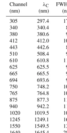
in-Table 1.Centroid wavelengths (λC) and bandwidth (full width at
half maximum, or FWHM) of GUVis channels.
Channel λC FWHM
(nm) (nm) (nm)
305 297.4 17.0
340 340.4 8.7
380 380.6 9.1
412 412.0 10.5
443 442.6 8.5
510 508.4 9.5
610 610.8 11.3
625 625.5 9.8
665 665.5 9.8
694 693.6 9.2
750 748.2 10.0
765 764.8 10.3
875 877.3 11.7
940 942.2 11.9
1020 1019.5 10.0
1245 1249.1 16.8
1550 1549.5 13.4
1640 1645.4 28.4
cludes channels with a centroid wavelength close to those of the AERONET Cimel and MFRSR instruments, as well as a number of additional wavelength bands. This wide spec-tral range and the ability to measure on a ship makes this instrument and its data products unique and will enable us to gain further insight into the properties and radiative effects of aerosol over the ocean.
The goals of this paper are threefold. First, we present the GUVis shadowband radiometer (Sect. 2) and the algo-rithms implemented at the Leibniz Institute of Tropospheric Research (TROPOS) for the data analysis (Sect. 3). This in-cludes the calculation of the spectral irradiance components including a motion correction for operation on ships and the subsequent retrieval of spectral AODs, Ångström coefficients and atmospheric water vapor column from the direct irradi-ance measurements (direct sun products). Secondly, an un-certainty analysis of these products is given based on theo-retical considerations (Sect. 4). Finally, a comparison is pre-sented with a Cimel sunphotometer over land and Microtops observations over sea, to confirm our accuracy estimates and the reliability of the products (Sect. 5). The paper ends with a discussion (Sect. 6), a summary and an outlook in Sect. 7.
2 Instrumentation
detec-Figure 1. The radiometer GUVis-3511 (center) with the BioSHADE accessory (right), which drives the shadowband. The BioGPS accessory is shown in the background on the left. The small white dome in the center of the radiometer top is the diffuser, which covers the filtered detectors.
tor (e.g., King and Myers, 1997). Exact values for the band-width and the centroid wavelength of each spectral channel are shown in Table 1. Each channel consists of interference and blocking filters (e.g., UG-11 and BG-25 bandpass filters from Schott) that are coupled to a “microradiometer” (Mor-row et al., 2010). Each microradiometer includes a photode-tector, preamplifier with three-stage gain, 24 bit analogue-to-digital converter, microprocessor and an addressable analogue-to-digital port. Data streams from all microradiometers are combined with measurements from ancillary sensors (e.g., temperature) and transmitted via a USB port to a PC. The design does not require to multiplex analogue signals from multiple photode-tectors, resulting in less electronic leakage and better relia-bility than traditional approaches. The instrument’s internal temperature is stabilized to 40±0.5◦C using a proportional– integral–derivative controller. Silicon photodiodes are used for channels with wavelengths up to 1020 nm, while channels above this wavelength use indium gallium arsenide detectors. Channels were selected from a list of standard wavelengths equipped with hard-coated ion-assisted deposition interfer-ence filters, which are known for excellent long-term stabil-ity. For the TROPOS instrument, three custom wavelengths were chosen to optimize the information content for atmo-spheric retrievals and had to be realized using less durable soft-coated interference filters for cost reasons. Specifically, this applies to the channels at 750 nm as absorption-free ref-erence for the 765 nm oxygen A-band channel, the 940 nm channel to measure the atmospheric water vapor column (Halthore et al., 1997) and the 1550 nm channel for cloud microphysics retrievals (Brückner et al., 2014). Data analy-sis suggests that the transmission of these soft-coated filters has changed significantly during the deployment of the in-strument (Sect. 4.1.2).
The filter microradiometer assemblies point at the center of an irradiance collector, which features a composite dif-fuser made of layers of generic and porous
polytetrafluo-Figure 2. Idealized irradiance time series measured during one shadowband sweep. When the sun is blocked, some part of the dif-fuse irradiance (black hatched area) is blocked by the shadowband in addition to the direct sun light. This part is estimated by extrap-olation of the data from the time series (blue line). The direct and diffuse irradiance is calculated from data obtained during the sweep. Between the sweeps, the global irradiance is observed.
roethylene (PTFE) sheets (Hooker et al., 2012). This design leads to relatively small cosine errors also in the infrared, where the scattering properties of traditional PTFE diffusers are typically degraded. The instrument is also equipped with two orthogonally mounted accelerometers for determining the instrument’s inclination (pitch and roll). The two sensors are not designed for use in a dynamically moving environ-ment, such as on ships, and measurement errors will occur when the instrument’s orientation is changing rapidly.
The radiometer is equipped with a computer-controlled shadowband accessory, called BioSHADE (Morrow et al., 2010). The band is made of black anodized aluminium, is 2.5 cm wide and has a diameter of 26.7 cm. Due to its ge-ometry, the shadowband occults a solid angle of 15◦of the sky from the sensor in zenith position. The width of the BioSHADE shadowband is broader compared to the MFRSR (3.3◦; Harrison et al., 1994) and the thin-cloud rotating shad-owband radiometer (TCRSR; 2 and 5◦; Bartholomew et al., 2011) and it is not feasible to measure the shape of the so-lar aureole for thin-cloud retrievals (Min and Duan, 2005). The uncertainty arising from the shadowband width on the calculation of the direct horizontal irradiance is discussed in Sects. 3.2 and 6.
The GUVis typically samples at 15 Hz at all times, includ-ing when a sweep is performed. For one sweep, the band rotates 180◦over the radiometer diffuser at a constant speed such that at least five data points are sampled during the time when all parts of the diffuser are shaded by the band. For measuring global irradiance, the band is stowed below the horizon of the instrument’s diffuser after one sweep during the split time to the next sweep. An idealized time series of one shadowband sweep is shown in Fig. 2. The method to de-rive the irradiance components from this kind of time series is described in Sect. 3.2.
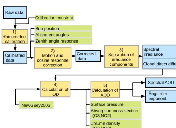
Figure 3.This flowchart outlines the data processing steps for the GUVis observations. Generated data products are shaded in blue, while calculation and processing steps are numbered and shaded in yellow. Supplementary data needed for processing are colored green.
stream. The GUVis is controlled by a data acquisition soft-ware running on a Windows laptop, which records the raw sensor signals and the irradiance plus additional status infor-mation in ASCII data files.
The instrumental setup is shown in Fig. 1. For operation the GUVis is mounted together with a total sky imager, which is used to identify sky conditions, and as supplementary in-formation for interpreting the irradiance measurements.
3 Method
Raw data are calibrated with calibration coefficients stored in the instrument’s internal memory. The calibration has been performed by the manufacturer and includes an absolute cal-ibration, a characterization of the sensor’s deviation from the desired cosine response and the determination of the spec-tral transmission of filters in the laboratory. These calibration data were shipped with the instrument and are used for our calculations and corrections.
For retrieving the direct irradiance and AOD, we have im-plemented several subsequent algorithms for data process-ing. These programs provide the separation of the irradiance components as well as the calculation of the spectral AOD. To achieve this, we use the proportionality of the direct hori-zontal spectral irradiance (DHI, I (λ)) to the spectral direct beam transmittance T (λ) expressed by the Beer–Lambert law (Beer, 1852), which is the fundamental relation also
ex-ploited by sunphotometer observations:
I (λ)=I0(λ) µ0
R2E exp(−maτ (λ)) , (1)
withma=µ−01and
T (λ)=I (λ) R
2
E
I0(λ) µ0
. (2)
The total spectral optical depth is denoted asτ (λ). For the top-of-atmosphere (TOA) solar irradianceI0at an earth–sun distance of 1 astronomical unit, the NewGuey2003 spectrum (Gueymard, 2004) is applied, which is convolved with the spectral response function of the GUVis channels obtained from the manufacturer’s instrumental characterization.I0is scaled by the inverse square of the actual sun–earth distance (RE, expressed in astronomical units), which is calculated
using equations given by WMO (2010). We assume the air mass factormato be equal to the inverse cosine of the zenith angleµ−01 here. The deviation from more complex expres-sions will be small as we are currently not using data with the sun close to the horizon (zenith angle>70◦; see Sect. 3.2).
steps of our data analysis are described. An outline of the processing is given by the flowchart shown in Fig. 3. 3.1 Motion and cosine error correction
Motion and cosine error corrections are applied simultane-ously before the actual processing because of their interde-pendency.
The motion correction compensates for the leveling errors of the instrument due to the ship movement and estimates the deviation from a horizontally aligned irradiance observa-tion. This is crucial because the spectral irradiance is defined either relative to a horizontal reference plane or a plane nor-mal to the solar beam. Due to the ship motion, the alignment of the instrument is changing continuously. This is compen-sated based on the method described by Boers et al. (1998). A correction factor (C1), according to Boers et al. (1998), is calculated from the ratio of the cosines of the true solar zenith angle (2) and the apparent zenith angle (2A), which is calculated from the sun position and the ship’s role, pitch and heading angles. The method from Boers et al. (1998) only corrects the direct irradiance component for the effects of motion and is thus only applicable when the sun is visible. Due to anisotropy in the diffuse radiation field, e.g., due to Rayleigh scattering, the diffuse component of irradiance also changes with the tilt of the sensor. ThereforeC1can be im-proved to account for the diffuse irradiance. By adapting the method of Boers et al. (1998) and using radiative transfer cal-culations, carried out with the libradtran package using the DISORT solver (Mayer and Kylling, 2005), improved cor-rection factors (C2andC3) are calculated. These factors are defined by Boers et al. (1998) as
C1(2, 2A)=
cos(2)
cos(2A)
, (3)
C2(2, 2A, λ)=
cos(2)+B(λ)
cos(2A)+B(λ)
, (4)
C3(2, 2A, λ)=
cos(2)+B(λ)·J (2, λ)
cos(2A)+B(λ)·J (2A, λ)
. (5)
where B=Idif(λ)/In(λ) is the ratio of the diffuse
(Idif(2, λ)) to direct normal irradiance at the surface (In(λ))
for 2= 0◦.J (2)=Idif(2, λ)/Idif(2=0◦, λ)is the diffuse
irradiance retrieved by radiative transfer calculations assum-ing a clear sky with only molecular scatterassum-ing (e.g., Rayleigh scattering) at the solar zenith angle, normalized to the dif-fuse irradiance at 2=0◦. The three correction factors are compared in Fig. 4 for the 305 and the 510 nm channels. For smaller wavelengths B is close to 1 and the diffuse ir-radiance becomes more dominant, and therefore C2 of the 305 nm channel deviates strongly from C1. Because of the stronger Rayleigh scattering, the diffuse irradiance at shorter wavelengths drops faster than the direct irradiance at lower sun elevation. Due to this effect, the deviation between C1 and C3 for channels with wavelengths around 305 nm has
the largest values for solar zenith angles between 60 and 70◦. The deviation is small and becomes less important for longer wavelengths due to the fact that Rayleigh scattering is almost negligible for wavelengths greater than 800 nm. Overall, ex-cept for short wavelengths around 300 nm, the deviation of the correction factorC1toC2andC3increases with decreas-ing sun elevation. Effects from aerosol are neglected in the radiative transfer calculations and the uncertainty resulting from this omission for the motion correction factorC3is in-vestigated in Sect. 4.1.1.
For measurements on the research vesselPolarstern, data from the ship’s marine inertial navigation system are used for motion correction. This system provides precise measure-ments of the roll, pitch and heading angles of the ship at high temporal resolution. Because the instrument is not perfectly aligned relative to the ship’s navigation system, we also apply a correction to account for this misalignment. This is done using the method of Bannehr and Schwiesow (1993), choos-ing data from clear days when the ship moves while the sun is either in the front, back or the sides of the ship. In these cases, the tilt correction is dependent on either the roll or the pitch angles alone. For land operation, the instrument’s po-sition is static, but this correction is also applied using the instrument’s internal accelerometer measurements to correct for slight misalignments of the setup. The internal measure-ments of pitch and roll angle have been calibrated using a precision level, and offsets relative to the diffuser are stored in the instrument and corrected by the firmware.
When observing an inclined collimated beam from a hor-izontal plane with an ideal detector, the measured signal changes with the cosine of the incident zenith angle. The cosine error correction removes the deviation of the instru-ment’s response for an inclined collimated incident beam of radiation from the ideal cosine response. The cosine error1c
of the instrument is taken from a lookup table provided by the instrument manufacturer using2Aaccording to the ship motion. This lookup table has been measured by the manu-facturer individually for all spectral channels as part of the instrument calibration. The cosine error correction factorCC is calculated using the method of Seckmeyer and Bernhard (1993):
CC(λ, 2A)=1c(λ, 2A) R(λ, 2A)
+1cD(λ) (1−R(λ, 2A)), (6)
with
cD(λ)=
R
2π1c(λ, 2A)cos(2A)d
R
2πcos(2A)d
, (7)
0 10 20 30 40 50 60 70 80 90
Solar zenith angle [ ]
0.4 0.2 0.0 0.2 0.4 0.6 0.8 1.0 1.2 1.4
Irradiance [no.]
(a) 305 nm
Rayleigh-diffuse irradiance
0.8 1.0 1.2 1.4 1.6 1.8 2.0 2.2 2.4 2.6
Correction-factor [no.]
Correction factors:
C1: direct only
C2: direct + isotropic diffuse
C3: direct + Rayleigh
0 10 20 30 40 50 60 70 80 90
Solar zenith angle [ ]
0.4 0.2 0.0 0.2 0.4 0.6 0.8 1.0 1.2 1.4
Irradiance [no.]
(b) 510 nm
Rayleigh-diffuse irradiance
0.8 1.0 1.2 1.4 1.6 1.8 2.0 2.2 2.4 2.6
Correction-factor [no.]
Correction factors:
C1: direct only
C2: direct + isotropic diffuse
C3: direct + Rayleigh
o o
Figure 4.Factors for motion correction measurements of the 305 and 510 nm GUVis channels. The two panels show the calculated diffuse irradiance (blue, leftyaxis), which is normalized to its maximum. The three correction factors are shown with respect to the rightyaxis, calculated for an inclination of 6◦of the ship towards the sun’s azimuth angle (e.g., high swell). The direct only (black solid) correction factor refers toC1described by Bannehr and Schwiesow (1993). The correction factorsC2(black dashed) andC3(red) are calculated taking
direct and diffuse irradiance into account. ForC2, an isotropic diffuse radiance distribution is assumed.C3is calculated assuming Rayleigh
scattering.
to be virtually independent of wavelength for the range from 305 to 765 nm and of the azimuth angle. Also at this stage, we do not use observations with the sun close to the horizon (solar zenith angle>70◦).
Assuming Rayleigh scattering to calculate the motion cor-rection factors (C3) is considered to be the most realistic and is used in the present algorithm, based on precalculated lookup tables varying2and2A. The cosine error correction factorCCis calculated from the lookup tables of the instru-mental cosine error obtained during calibration. Therefore, the correction of the observed irradiance (Im(λ)) to the
cor-rected irradiance (IC(λ)) for our processing is defined as
IC(λ)=Im(λ)
C3(λ, 2, 2A)
CC(λ, 2A)
. (8)
3.2 Separation of irradiance components
To calculate the irradiance components, the data of each shadowband sweep are analyzed separately. The irradiance is measured with a sampling frequency of 15 Hz during the sweeps. With this temporal resolution, even short-term irra-diance fluctuations can be resolved. The global irrairra-diance is observed at the start and end of a shadowband sweep, when the shadowband is outside the field of view of the sensor. The minimum irradiance determined during the sweep cor-responds to the time when the diffuser is completely shaded by the shadowband, if the sun is visible. If no clear minimum is identified, the direct irradiance is very small or negligible, and only the global irradiance is determined by the algorithm. The difference of the global irradiance and the minimum irradiance measured during the sweep represents the direct
component of irradiance, together with an additional diffuse part blocked by the shadowband. Figure 2 shows an ideal-ized time series for one sweep (red). The shadowband is de-signed to block the sun completely for at least five samples of the irradiance. The hatched area represents the blocked diffuse irradiance during the sweep. This occurs because the shadowband blocks a significant part of the sky in addition to the sun. To estimate the amount of blocked diffuse ir-radiance, 30 data points before and after the transit of the shadow across the diffuser are used to extrapolate the dif-fuse irradiance for the time when the minimum irradiance is detected (blue line). Values from both extrapolations are averaged. With this information, we can calculate the direct irradiance as the difference between this extrapolated value and the minimum irradiance (Morrow et al., 2010).
It is possible that thick clouds obscure the sun during one sweep. In this case, the data of the sweep will show mul-tiple minima or fluctuations. This behavior is identified by the algorithm and in these cases only the global irradiance is observed. Nevertheless, in situations with thin clouds (e.g., the sun is still visible when obscured by the cloud), the fluc-tuations are small and processing of the data is still possi-ble. The uncertainty for the retrieved direct irradiance from sweeps with fluctuations in the irradiance data is investigated in Sect. 4.1.3.
0 10 20 30 40 50 60 70 80 Solar zenith angle [ ]
0.05 0.10 0.15 0.20 0.25 0.30 0.35 0.40 0.45
AOD
(a) 305 nm
0 10 20 30 40 50 60 70 80
Solar zenith angle [ ] 0.05
0.10 0.15 0.20 0.25 0.30 0.35 0.40 0.45
AOD
(b) 510 nm
<-2 0 2 4 6 8 >10
Motion correction error [%]
o o
Figure 5.Relative errors in the motion correction for the 305 and 510 nm channel of the GUVis radiometer by not taking aerosols into account. The error is calculated by comparing correction factorC3 calculated with no aerosol to correction factors with added aerosol. These correction factors have been calculated likeC3, but using radiative transfer calculations with aerosol type and properties according to Shettle
(1990) with AODs of 0.05 to 0.45. The calculations are done for an inclination of 6◦of the ship towards the sun’s azimuth angle (e.g., high swell).
sun has to be investigated in further work. Preliminary radia-tive transfer calculations for different aerosol conditions and various solar zenith angles show that the uncertainty from this extrapolation is around 1 % for most conditions with the sun elevated more than 30◦ above the horizon. This uncer-tainty may increase when the aerosol has strong forward scat-tering (eg. desert dust). Nevertheless, an uncertainty of 1 % agrees with the estimation of the “edge-shadow voltage un-certainty” for less variable sweeps observed by Miller et al. (2004). At this stage, we do not use observations with the sun close to the horizon (solar zenith angle>70◦).
3.3 Calculation ofτ
From the observed spectral values of DHI, the correspond-ing total optical depthτTof the atmosphere can be calculated from Eq. (1). The total optical depth τT is composed of the optical depths for Rayleigh scattering τR, trace gas absorp-tion τG and aerosol extinctionτA. In the present algorithm, the gas absorptionτGtakes into account absorption by ozone and NO2for all channels, plus H2O, CO2and CH4for chan-nels matching the AERONET Cimel sunphotometer (940, 1020 and 1640 nm). The AOD,τA, can then be determined by subtracting τR (for Rayleigh scattering) andτG fromτT obtained from the measurements.
τA(λ)=τT(λ)−τG(λ)−τR(λ) (9)
In the following, we describe the calculation of τRand the individual components ofτG.
3.3.1 Calculation ofτR
To calculateτR, we have selected the method from Bodhaine et al. (1999), which takes pressure (P), CO2 concentration
(CO2) and the gravitational acceleration depending on lati-tude and altilati-tude into account. A current CO2global mean concentration of 400 ppm is assumed and local pressure ob-servations are used. The uncertainty ofτRis related to the uncertainty of the observed air pressure (see Sect. 4.2.1). 3.3.2 Calculation ofτO3 andτNO2
Given the columnar number concentrationsn (m−2) of O3 and NO2,τO3 andτNO2 of these trace gases are calculated as
τO3=σO3n, (10)
τNO2=σNO2n. (11)
σ denotes the absorption cross section (m2) of the gases and are taken from Schneider et al. (1987) for NO2 and (Serdyuchenko et al., 2014) for O3. Daily values of the columnar number concentration are obtained from the Aura Ozone Monitoring Instrument (AURA-OMI) satellite data (McPeters et al., 2008; Bucsela et al., 2013). The uncertain-ties ofτO3 andτNO2 are related to the uncertainty of the
ob-served columnar number concentrations measured by satel-lites (see Sect. 4.2.2).
3.3.3 Calculation ofτCH4 andτCO2
For obtaining the absorption contribution of CH4 and CO2 toτG, estimates are obtained similarly to the sunphotome-ter processing by AERONET1. The absorption of CO2 influ-ences observations in both the 1550 and the 1640 nm chan-nel, while the latter is also affected by CH4absorption. Based on computations using the standard US 1976 atmospheric 1http://aeronet.gsfc.nasa.gov/new_web/Documents/version2_
model for the 1640 nm channel, τCH4 was set to 0.0036
and τCO2 to 0.0089 at a standard atmospheric pressure P0
of 1013.25 hPa for the 1640 nm channel. The τCO2 for the
1550 nm channel was set to 0.0007.τCH4 andτCO2 are then
scaled with the actual air pressureP byPP
0. The uncertainties
of τCH4 andτCO2 are therefore related to the uncertainty of
the measured air pressure (see Sect. 4.2.3). 3.3.4 Calculation ofτw
The 940 nm channel is used to retrieve the precipitable wa-ter using a logarithmic transformation of the measured di-rect beam transmittance (Smirnov et al., 2004), where co-efficients a andb in the following equation are instrument specific constants and are linked to the filter response of the instrument (Pérez-Ramírez et al., 2014). We have chosen to obtain these coefficients from a fit of the shadowband ra-diometer data to the precipitable water (w) obtained from the Cimel instrument by cross calibration.
The following equation is used to model the atmospheric transmissionT940in this channel:
T940=T940,GT940,RT940,AT940,w. (12)
Here,T940is the measured total atmospheric transmission at 940 nm. The transmissions from gas absorption (T940,G) and Rayleigh scattering (T940,R) are calculated using the methods described in the previous subsections. The transmission from aerosol (T940,A) and water vapor (T940,w) is unknown at this stage.
T940,A can be expressed from Eq. (2) as T940,A= exp−µ−01τA(940 nm)
and estimated using the Ångström exponent calculated from the 440 and 870 nm channels.
To modelT940,w, the following equation is used:
T940,w=exp
−a(w mw)b
. (13)
T940,w depends on two channel-specific coefficientsaandb and the relative air mass factor for water vapormw, which is calculated using the method of Kasten (1965).
Equation (12) can be reformulated as a linear equation of the coefficientsaandb:
ln
ln T
940,AT940,RT940,G T940
=ln(a)+bln(w mw) . (14) From Eq. (14) we have determined values ofa=0.6131 and b=0.6712 to best match the precipitable water w re-trieved from the Cimel instrument by least-square regression. With this approach, we avoid the use of spectroscopic data together with the filter response to establish the link between precipitable water and spectral direct beam transmittance. The advantage is that this ensures the consistency with the AERONET observations and allows us to monitor changes in the transmittance of the unstable 940 nm filter using collo-cated AERONET observations, which are routinely available
at our institute. Due to the fast change of the filter character-istics, it is desirable to carry out these parallel observations frequently, in particular before and after measurement cam-paigns.
The retrieved precipitable water is related linearly toτw at 1640 and 1020 nm to account for the water absorption in these channels (Schmid et al., 1996; Michalsky et al., 1995).
τw(1640 nm)=0.0014·w−0.0003 (15) τw(1020 nm)=0.0023·w−0.0002 (16) Due to the reliance of this method on Cimel observations, we cannot estimateτwfor the 1550 nm channel with this ap-proach. We are planning to derive the relation betweenτw and precipitable water from spectroscopic data for all GUVis channels affected by water vapor absorption in the future.
Comparing the results obtained with our method and the GUVis instrument to the AERONET derived precipitable wa-ter, a linear regression shows close agreement, with a slope of 1.001 and a standard deviation of 0.029 cm. Therefore, we conclude that this method is reliable as long as the calibration and filter response of the 940 nm channel remains stable or collocated AERONET measurements are regularly used for cross calibration. The uncertainty forτwis estimated from a comparison with the retrievals from the Cimel sunphotome-ter (see Sect. 4.2.3).
3.4 Cloud mask and quality control
total sky camera in synergy with the GUVis instrument can improve the clear sky identification in future work.
4 Uncertainty estimation
Estimates of the combined uncertainties of the GUVis obser-vations with respect to the observation of spectral horizontal irradiance and the estimation of the AOD are presented in this section.
Uncertainties resulting from the different sources of er-ror are discussed in the following subsections. The combined relative uncertainty of the direct horizontal irradiance (1IT)
is calculated from its individual contributions as follows:
1IT =
q
1I2
an+1Imot2 +1Ical2 . (17)
The uncertainty of the motion correction (1Imot, see Sect. 4.1.1) is taken from a precalculated lookup table, and the calibration uncertainty (1Ical, see Sect. 4.1.2) was esti-mated from the change in responsivities between two consec-utive calibrations (the change was smaller than±2 % for all stable channels). The uncertainty caused by amplifier noise (1Ian, see Sect. 4.1.3) is calculated during the processing from the uncertainty of the fit parameters.
Table 3 summarizes the total estimated uncertainty for land and shipborne operation. As mentioned in Sect. 4.1.2, the responsivity of some channels has been found to change significantly and is excluded from the further uncertainty analysis. For the three channels (305, 340 and 380 nm), this issue should be fixed for future measurements due to the modification of the instrument mentioned in Sect. 4.1.2. All other channels show an uncertainty between about 2.5 and 4 % within a 95 % confidence interval for the irradiance mea-surements on land and ship, respectively.
Due to the logarithmic dependency ofτ toI from Eq. (1), the uncertainties of the direct horizontal irradiance (IT1IT)
and the extraterrestrial irradiance (I01I0) are combined and translated to the absolute uncertainty1τ as follows:
1τ =µ0
s
1IT
IT
2 +
1I0
I0 2
. (18)
After all uncertainty components are calculated, the1τA sums up all components:
1τA=
q
1τ2+1τ2
R+1τG2. (19)
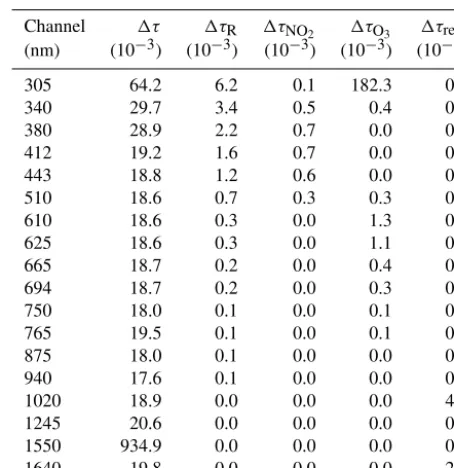
The equation includes the contribution of Rayleigh scat-tering (1τR) and gas absorption (1τG), which in turn in-cludes the absorption from O3, NO2, H2O, CH4 and CO2. The contribution of each component of1τ is shown in Ta-ble 2. TaTa-ble 3 shows the estimated total uncertainty for the AOD calculations in absolute values for each stable channel. The uncertainty of AOD is less than 0.02 for all channels.
As we investigate the uncertainty of atmospheric transmis-sion (T 1T) for comparison to sunphotometers later,T 1T
can be related to the uncertainty of the direct horizontal ir-radiance (I 1I) and the absolute uncertainty of the atmo-spheric optical depth (1τ) of the GUVis as follows from Eq. (1):
1I= dI
dT 1T = I0µ0
RE2 1T , (20)
1τ= dτ
dT 1T = −µ0 1T
T . (21)
4.1 Irradiance uncertainties
In the following, sources of uncertainties are presented which influence the direct irradiance measurement.
4.1.1 Uncertainty of the motion correction
The motion correction factorC3described in Sect. 3.1 takes Rayleigh scattering but no aerosol into account (AOD=0). Calculations with aerosol require knowledge of aerosol opti-cal properties (e.g., size distribution, single scattering albedo, asymmetry parameter, optical depth) which we only can guess at this stage of processing. To avoid time-consuming radiative transfer calculations during the processing, aerosol is neglected completely for the motion correction. To esti-mate the uncertainty due to this omission, we have calcu-lated correction factors using radiative transfer calculations taking aerosol with properties according to Shettle (1990) into account. The default properties are a rural type aerosol in the boundary layer, background aerosol above 2 km, spring-summer conditions and a visibility of 50 km. For our calcula-tions, the AOD is modified in the range of 0.05 to 0.45 com-paring those correction factors toC3 without aerosol. Fig-ure 5 shows the deviation ofC3calculated with and without aerosol influence for the 305 and the 510 nm channels for
2A=2– 6◦(e.g., high swell). For a smaller difference be-tween2and2A(e.g., lower swell), the error will be reduced and turn negative when2A> 2.
From these calculations, we estimate the motion correc-tion uncertainty, forcing the AOD to be 0.45, which is a high AOD and rarely observed over ocean. Also, the sky is as-sumed to be cloud free. The uncertainty is taken from pre cal-culated lookup tables depending on2Aand2. At the recent Polarsterncruise PS83 the swell conditions were calm for the most time (see Fig. 8), which is defined as misalignment of the ship smaller than 5◦. The mean uncertainty contribu-tion of the mocontribu-tion correccontribu-tion to the irradiance measurements from this cruise was about 0.3 % for all channels.
Table 2.Mean absolute uncertainty of retrievedτfrom the our scheme, originating from the measured irradiance (1τ), as well as Rayleigh scattering (1τR), NO2absorption (1τNO2), O3absorption (1τO3) and the combination of H2O, CH4and CO2absorption (1τrem).
Channel 1τ 1τR 1τNO2 1τO3 1τrem
(nm) (10−3) (10−3) (10−3) (10−3) (10−3)
305 64.2 6.2 0.1 182.3 0.0
340 29.7 3.4 0.5 0.4 0.0
380 28.9 2.2 0.7 0.0 0.0
412 19.2 1.6 0.7 0.0 0.0
443 18.8 1.2 0.6 0.0 0.0
510 18.6 0.7 0.3 0.3 0.0
610 18.6 0.3 0.0 1.3 0.0
625 18.6 0.3 0.0 1.1 0.0
665 18.7 0.2 0.0 0.4 0.0
694 18.7 0.2 0.0 0.3 0.0
750 18.0 0.1 0.0 0.1 0.0
765 19.5 0.1 0.0 0.1 0.0
875 18.0 0.1 0.0 0.0 0.0
940 17.6 0.1 0.0 0.0 0.0
1020 18.9 0.0 0.0 0.0 4.8
1245 20.6 0.0 0.0 0.0 0.0
1550 934.9 0.0 0.0 0.0 0.0
1640 19.8 0.0 0.0 0.0 2.9
Table 3.Summary of the main results of our evaluation of the GUVis shadowband radiometer. The relative change in calibration of each channel is shown in column two. Channels with soft-coated filters (750, 940, 1550 nm), and channels affected by a change in transmission of a diffuser insert (305, 340, 380 nm) are excluded from the uncertainty estimate. The mean uncertainty and deviation according to a 95 % confidence interval from our analysis (Sect. 4) are shown for the spectral irradiances for all stable channels for land-based and shipborne observations in columns three and four. The mean uncertainty for the calculation of AOD is shown in absolute values in columns five and six. The linear regression parameters obtained from the comparison of GUVis with Cimel (land-side) and Microtops (shipborne) spectral direct beam transmittance observations are given in the columns 7 to 9 and 10 to 12, respectively.
1 2 3 4 5 6 7 8 9 10 11 12
Channel Calibration 1IT 1τA Comparison to Cimel Comparison to Microtops
deviation land ocean land ocean slope σ R slope σ R
(nm) (%) (%) (%) (10−2) (10−2) (–) (–) (–) (–) (–) (–)
305 28.0 – – – – – – – – – –
340 10.9 – – – – 1.019 0.006 0.998 – – –
380 2.2 – – – – 1.003 0.008 0.998 1.026 0.029 0.971
412 0.6 2.6 4.4 1.8 2.0 – – – – – –
443 2.0 2.5 4.6 1.8 2.0 0.966 0.010 0.997 1.004 0.024 0.967
510 0.6 2.5 3.8 1.8 2.0 1.057 0.013 0.994 1.040 0.028 0.975
610 0.7 2.4 3.7 1.8 2.0 – – – – – –
625 0.7 2.5 3.7 1.8 2.0 – – – – – –
665 0.6 2.5 3.7 1.8 2.0 1.028 0.015 0.987 1.029 0.026 0.958
694 0.1 2.5 3.8 1.8 2.0 – – – – – –
750 18.4 – – – – – – – – – –
765 1.4 2.8 4.0 1.7 1.9 – – – – – –
875 1.6 2.5 4.1 1.7 1.9 1.014 0.019 0.961 0.987 0.026 0.974
940 9.2 – – – – – – – – – –
1020 1.2 2.5 4.1 1.9 2.1 1.002 0.015 0.965 – – –
1245 0.4 2.8 5.0 1.8 2.0 – – – – – –
1550 40.4 – – – – – – – – – –
4.1.2 Uncertainty of the calibration and extraterrestrial spectrum
The instrument was calibrated by the manufacturer at the time it was built. It was recalibrated after two years to verify the stability of the instrument. For these calibrations, NIST-traceable 1000 Watt FEL standard lamps have been used. Table 3 shows the deviation of the calibration constants be-tween both calibrations. Most channels show a drift of less than 2 %, which is within the expected range for the tempo-ral drift of such an instrument and agrees with the findings of Schmid and Wehrli (1995) for laboratory calibrations. Addi-tionally, a Langley calibration was performed on clear days at sea level in San Diego after the recalibration to verify the calibration from the laboratory. Solar measurements for Lan-gley calibrations from sea level causes uncertainties due to fast changing conditions in the boundary layer, also the ex-traterrestrial spectrum is not known to be better than 3.5 % for wavelengths below 400 nm and 0.8 % above (Gueymard, 2004). For channels with hard-coated filters and wavelengths of up to 875 nm, differences between lamp-based and Lan-gley calibrations differed between 0 and 5 %. For channels with wavelengths between 1020 and 1640 nm the difference was 5 to 6 %. Considering that the Langley calibration was performed at sea level under far from ideal conditions, the agreement can be considered good.
A Langley calibration on a high-altitude site for this in-strument is desirable and will be done in future. This will decrease the calibration uncertainties to about 1 % (Schmid and Wehrli, 1995). The drift of the spectral filters will be in-vestigated with ongoing laboratory calibrations in the future. The channels at 305, 340 and, to a lesser extent, at 380 nm show large drifts. These have been attributed to a change in the transmission of a special insert below the instrument’s main Teflon diffuser, which is necessary to get an adequate cosine response at wavelengths larger than about 800 nm. BSI has addressed this problem by replacing this insert with a new material in our GUVis instrument. Hence, the stability of these channels should have significantly improved, which nevertheless needs to be verified by future calibrations.
The channels at 750, 940 and 1550 nm also show large deviations. They correspond to the custom channels chosen by TROPOS as mentioned in Sect. 2. These channels use soft-coated interference filters for cost reasons, which have a known lower temporal stability than hard-coated ones, as is confirmed by these findings. In future, the filters could be replaced by hard-coated filters to increase the stability of these channels. At this stage, no replacement of filters is planned for our instruments, and a small calibration uncer-tainty can only be achieved by frequent calibrations. For the 940 nm channel, this can be realized by cross calibration with AERONET observations in the field, as outlined in Sect. 3.3. The optical depth calculated from Eq. (1) can only be as certain as the TOA irradianceI0is known. In our process-ing the extraterrestrial spectrum “NewGuey2003”
(mard, 2004) is used. The uncertainty estimate from Guey-mard (2004) range from 3.5 % in the 280–400 nm band to 0.8 % in the 700–1000 nm band. The uncertainty related to each channel of the GUVis is propagated through our pro-cessing causing a mean uncertainty of AOD of 0.008 for the 510 nm channel. Absolute mean values for this uncertainty for all channels are presented in Table 2.
4.1.3 Uncertainty caused by amplifier noise
Noise in the electrical amplifiers of the radiometer directly affects the accuracy of the radiation measurements. We have attempted here to estimate the amplitude for each channel, using measurements obtained during the absolute calibration in the laboratory. The amplitude is assumed to be constant for different levels of incident radiation. High-frequency fluctu-ations in the direct beam transmittance during observfluctu-ations will introduce a similar uncertainty during our processing. Both effects are combined in the following uncertainty anal-ysis.
The uncertainty due to amplifier noise is strongly reduced by averaging, which is in fact done several times by our method for separating the different irradiance components. The global irradiance is measured and averaged for 20 s (300 samples) between two sweeps, resulting in negligible uncertainty. The direct irradiance is, however, estimated us-ing a smaller number of measurement values. First, a mean ir-radiance is calculated while the diffuser is completely shaded from direct sun from at least five samples for clear sky, low AOD and high sun conditions and more than 10 samples for lower sun, which again reduces the influence of noise. Sec-ondly, the shading of diffuse irradiance is estimated from the sweep data by linear extrapolation using 30 observations be-fore and after the transit of the shadow across the diffuser. The uncertainties of the fit parameters are also calculated, which allow us to determine the uncertainty of the extrapo-lated values, and are attributed here to the influence of noise. Please note that deviations from the underlying assumption of the linear model could also arise for other reasons, such as variations of the forward scattering peak, e.g., expected for large particles such as dust or ice crystals.
The uncertainty for the DHI during the Melpitz Column experiment (see Sect. 5 for a brief description) does not ex-ceed 0.6 % within a 95 % confidence interval. Since the dif-fuse irradiance is calculated as the difference of the global and the direct irradiance, and the uncertainty of the global irradiance due to measurement noise is negligible, its uncer-tainty is set to be equal to that for the direct irradiance.
4.2 AOD uncertainties
4.2.1 Uncertainty ofτR
Since the calculationτRis directly proportional to the pres-sure, the absolute uncertainty1τRis given as
1τR=τR
1P
P . (22)
1P is defined by the manufacturer of the weather station Lufft as±5 hPa≈0.5 %.
This method assumes a current CO2 concentration of about 400 ppm, which can vary over time. However, the de-viation ofτRfor varying CO2concentration of up to 40 ppm difference is only about 0.003 % and therefore negligible.
Absolute mean values for this uncertainty are presented in Table 2.
4.2.2 Uncertainty ofτO3andτNO2
Because of the spectral dependence of absorption, trace gases introduce a wavelength-dependent uncertainty in the calcu-lation of AOD. This uncertainty is mainly determined by the uncertainty of the trace gas column density, which is obtained here from satellite retrievals by the AURA-OMI instrument. The uncertainty of the column density of O3is set to 3 % and for NO2column density to 20 %, as specified in the OMI al-gorithm theoretical basis documents (Bhartia, 2002; Chance, 2002) and confirmed by evaluations (McPeters et al., 2008; Bucsela et al., 2013). These uncertainties are directly trans-lated into an uncertainty ofτG, with different importance for different channels due to the wavelength dependence of both aerosol properties and gas absorption. Absolute mean values for this uncertainties are presented in Table 2.
4.2.3 Uncertainties of remaining gas absorption The precipitable water is calculated using the 940 nm chan-nel measurements in Eq. (14). From the linear regression of precipitable water derived from both the Cimel and GUVis we have found the standard deviation σw to be 0.029 cm.
From the AERONET sample data uncertainty estimate (Hol-ben et al., 1998) we calculate the standard deviation as
σC= 0.017 cm. From these values we estimate the combined
uncertainty of precipitable water1wobserved with the GU-Vis as
1w=
q
σ2
w+σC2=0.034 cm. (23)
Using this equation, we calculate the uncertainty 1τw for the 1020 and 1640 nm channel from Eqs. (15) and (16) as1τw(1020 nm) = 7.82×10⁻⁵and1τw(1640 nm) = 4.76× 10⁻⁵.
τCO2 and τCH4 are scaled to the ambient
pres-sure and applied only to the 1640 nm channel. There-fore, the uncertainties 1τCO2 and 1τCH4 can be
cal-culated from the uncertainty of the pressure measure-ments, which are assumed to have a value of 1P= 5 hPa.
This leads to errors of1τCO2(1640 nm) = 4.361×10
−5 and
1τCH4(1640 nm) = 1.764×10
−5, respectively.
The uncertainty (1τrem) for the absorption of CO2, CH4 and precipitable water is combined as follows for the 1640 nm channel:
1τrem=
q
(1τCO2)2+(1τCH4)2+(1τw)2. (24)
Absolute mean values for this combined uncertainty are pre-sented in Table 2.
5 Evaluation
The Melpitz Column experiment took place between May and July 2015 in a rural area at the TROPOS measurement site Melpitz near Leipzig in Germany. During this time a va-riety of aerosol and boundary layer measurements were con-ducted to investigate the aerosol distribution in the whole tropospheric column. To verify the reliability of the GU-Vis shadowband radiometer, it has been deployed during the Melpitz Column field experiment on land together with a Cimel sunphotometer participating in the AERONET net-work, which allows a direct comparison of the observations and products.
As the main strength of the GUVis is its ability to be op-erated on ships, measurements during the cruise PS83 with the RVPolarsternare also analyzed here and are compared to MAN observations with a Microtops sunphotometer. 5.1 GUVis vs. Cimel observations
To verify our estimate of the uncertainty of the GUVis in-strument as discussed in the previous section, we have op-erated the instrument in close vicinity of an AERONET Cimel sunphotometer during the Melpitz Column campaign. AERONET sunphotometers have a very strict calibration and quality assurance protocol and are thus used as reference ob-servations here. On land, when stabilization is not an issue, sunphotometers are also the preferred method for aerosol characterization due to the fact that the direct normal and not the direct horizontal irradiance is measured. Firstly, this results in a better signal-to-noise ratio particularly at low sun elevations. Secondly, the separation of irradiance com-ponents is avoided, which introduces an additional uncer-tainty in the data analysis of shadowband radiometer mea-surements. Comparing both instruments is a good benchmark to test the reliability of the shadowband radiometer observa-tions and the derived data products.
0.0 0.2 0.4 0.6 0.8 1.0 0.0
0.2 0.4 0.6 0.8 1.0
y = 1.002x + 0.000
σ1 = 0.015
y = 0.980x + 0.019
σ2 = 0.015
R = 0.965 N = 1468
(a) T (1020 nm)
0.0 0.2 0.4 0.6 0.8 1.0
0.0 0.2 0.4 0.6 0.8 1.0
y = 1.057x + 0.000
σ1 = 0.013
y = 1.063x + -0.004
σ2 = 0.013
R = 0.994 N = 1468
(c) T (500/510 nm)
0.0 0.2 0.4 0.6 0.8 1.0
0.0 0.2 0.4 0.6 0.8 1.0
y = 1.019x + 0.000
σ1 = 0.006
y = 1.035x + -0.004
σ2 = 0.006
R = 0.998 N = 1468
(e) T (340 nm)
0.0 0.2 0.4 0.6 0.8 1.0
0.0 0.2 0.4 0.6 0.8 1.0
y = 0.921x + 0.000
σ1 = 0.011
y = 0.822x + 0.007
σ2 = 0.010
R = 0.998 N = 1468
(b) AOD (1020 nm)
0.0 0.2 0.4 0.6 0.8 1.0
0.0 0.2 0.4 0.6 0.8 1.0
y = 0.819x + 0.000
σ1 = 0.020
y = 0.924x + -0.027
σ2 = 0.016
R = 0.998 N = 1468
(d) AOD (510 nm)
0.0 0.2 0.4 0.6 0.8 1.0
0.0 0.2 0.4 0.6 0.8 1.0
y = 0.949x + 0.000
σ1 = 0.025
y = 1.042x + -0.039
σ2 = 0.017
R = 0.998 N = 1468
(f) AOD (340 nm)
30 35 40 45 50 55 60 65 70
Zenith angle [ ]
Transmittance CIMEL
Transmittance GUVis
AOD GUVis
AOD CIMEL
o
Figure 6.Comparison of the spectral direct beam transmittance (left panels) and spectral AOD (right panels) for three matching channels of the GUVis and Cimel instruments. The parameters of the linear regressions with intercepts forced through zero (first equation) and free intercept (second equation) are denoted in each panel. The deviations from the regression lines are denoted asσ1andσ2.Rdenotes the
correlation coefficient andNthe number of available measurement points for comparison. The points are colored with respect to the zenith angle.
to the instrumental measurements. Specifically, the nonlin-earity introduced by the Beer–Lambert law and processing uncertainties in Rayleigh scattering and gas absorption are avoided.
T has been calculated from Eq. (2). For GUVis obser-vations, we calculate T directly form the observed DHI. For Cimel observations, the retrieved τT as reported by AERONET has been used to calculate the corresponding values of T. The comparison shows a robust linear behav-ior with increasing deviations for longer wavelengths. The slopes are close to the ideal value of unity for most channels, with a difference below 3 %, except for the 443 and 510 nm channels, which exhibit deviations of about 3.4 and 5.7 %, respectively.
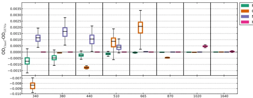
Figure 7 comparesτRandτG obtained from our scheme and the AERONET processing to identify resulting
differ-ences in the retrievals. Here, our retrieval is applied for the central wavelengths given by the Cimel sunphotometer to concentrate on the inherent method differences. The figure shows only small difference of gas absorption optical depths between both algorithms, except for ozone in the 340 nm channel. In general, the differences inτ of both instruments can be explained due to the input data used for calculations. While AERONET uses climatological means for the gas col-umn density of ozone and NO2, we rely on satellite products from the AURA-OMI satellite instrument.τR also shows a minor difference due to deviations of the air pressure mea-surements. Due to the large wavelength dependence of ozone absorption around 340 nm, the calculated τO3 strongly
340 380 440 510 665 870 1020 1640 0.0015
0.0010 0.0005 0.0000 0.0005 0.0010 0.0015 0.0020 0.0025 0.0030 0.0035
OD
Cim
el
-O
D
GUV
is
Ray O3 NO2 H2O
340 380 440 510 665 870 1020 1640
Wavelength [nm] 0.010
0.009 0.008 0.007
Figure 7.Comparison of the calculated meanτand its components for matching channels during the Melpitz Column campaign. Shown is the difference of the optical depth components retrieved by AERONET with the Cimel sunphotometer (ODCimel) and GUVis (ODGUVis) in a box and whisker plot. The median is displayed; the box extends to the 25th percentile and the whiskers towards the 75th percentile of the data. Shown are the optical depth for Rayleigh (Ray), ozone (O3), nitrogen dioxide (NO2) and water vapor (H2O). To highlight the
differences in the retrieval scheme, we have adjusted the central wavelengths of the GUVis channels to those of the Cimel instrument. The yaxis is split to include the large difference of the 340 nm ozone optical depth.
(341.5 nm) is smoothed out in the GUVis processing. There-fore a large difference ofτO3is observed for this channel.
Accepting these minor differences, the robust linear be-havior shown in Fig. 6 assures us that both instruments pro-vide comparable products, and the deviation from the regres-sion line1T can be translated from Eq. (20) into a measure-ment deviation for both the direct horizontal irradiance (1I) and atmospheric optical depth (1τ) of the GUVis, using the observations from the Cimel instrument as reference.
This deviation has been calculated for different situations in the atmosphere (e.g., only marine aerosol, desert dust or continental aerosol). Values for the typical AOD were chosen using the classification scheme from Toledano et al. (2007), and the deviation was estimated using the standard deviation of the direct beam transmittance obtained from the compari-son of both instruments. The deviations show a similar mag-nitude to uncertainties obtained from theoretical arguments in Sect. 4. It also shows that the uncertainty is strongly depen-dent on the observation conditions, specifically the aerosol loading and sun elevation.
5.2 GUVis vs. Microtops II observations
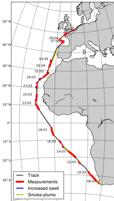
The German research vesselPolarsternis an ice breaker op-erated by the Alfred Wegener Institute and mainly intended for polar research. In autumn and spring of each year, tran-sit cruises take place across the Atlantic Ocean for trans-ferring the ship into the corresponding polar summer hemi-sphere. Since 2007, these transit cruises are used to carry out atmospheric measurements within the framework of the OCEANET project (Macke, 2009). During the cruise PS83 in spring 2014, the GUVis shadowband radiometer was op-erated for the first time as part of OCEANET, with the aim of
providing automated measurements of aerosol optical prop-erties and its radiative effects. The track of this cruise is shown in Fig. 8.
Maritime aerosol consisting of sea salt, sulfate and water was observed throughout the cruise. Continental influences were insignificant in the Southern Hemisphere but became more prominent in the Northern Hemisphere. Mineral dust aerosol as well as biomass burning aerosol was observed while passing along the African coast west of the Saharan desert from 17 until 27 March 2014.
The shadowband radiometer was installed on the naviga-tion deck of the ship as far away as possible from the ship’s superstructures to minimize shading effects. Only the mast and chimney as well as the smoke plume of the ship were able to shade the sensor under certain geometries and wind conditions.
Sunphotometer observations with Microtops instruments were also taken during the cruise PS83 as a contribution to the MAN by scientists from the Max Plank Institute of Me-teorology (Smirnov et al., 2009). These measurements were carried out manually every 10 to 15 min during clear sky con-ditions and include five spectral channels ranging from 380 to 870 nm. The handheld photometer is manually pointed to-wards the sun, taking a sequence of 10 measurements. Be-fore each measurement, the sky condition is checked by eye to be cloud free and to minimize the influence of the ship’s smoke plume. Since the Microtops is a handheld instrument, the smoke plume can be avoided by selecting another posi-tion on the ship for the measurement, in contrast to the fixed position of the GUVis instrument.
30°S 20°S 10°S 0° 10°N 20°N 30°N 40°N 50°N
0° 10°E 20°E 30°E 40°W 30°W 20°W 10°W
08:03 10:03 12:03 14:03 16:03 18:03 23:03
25:03 27:03
29:0331:03 02:04
04:04 07:04 09:04
11:04
Track Measurements Increased swell Smoke-plume
Figure 8. The track for cruise PS83 of the research vessel
Po-larstern. Track points with observations available from both the
GUVis and Microtops instruments are marked in red. Additionally, high-swell conditions during the cruise are marked blue, and a pos-sible influence of the ship’s smoke plume on GUVis observations is marked in yellow.
protocol as for AERONET Cimel sunphotometers (Smirnov et al., 2002). The data are available from the website of the Goddard Space Flight Center of NASA and are used here as reference for the shadowband radiometer measurements.
The alignment information for the motion correction of the GUVis instrument is taken from the ship’s marine inertial navigation system. This system provides precise measure-ments of the roll, pitch and heading angles with high tempo-ral resolution. Detailed meteorological data are also available from the ship’s weather station and can be obtained from the DSHIP database system.
For quality assurance, quality flags were added to the ob-servational data for different conditions. To investigate the influence of the smoke plume of the ship on the measure-ments, the relative wind speed and direction was used to-gether with the sun position to determine the likelihood of the smoke plume passing between the sun and the shadowband
radiometer sensor. Also, the deviation of the ship from hori-zontal due to the swell was used for a quality flag. Data with a misalignment of 5◦and higher are marked as high swell. Due to larger misalignments of the ship caused by higher swell, the uncertainty of the misalignment correction is expected to increase as described in Sect. 4.1.1.
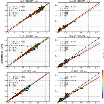
The comparison shown in Fig. 9, as well as the regression parameters quoted in Table 3, shows an overall agreement of the spectral direct beam transmittance observations from both instruments with a deviation below 4 %, which is in the same range as the comparison to the Cimel sunphotometer. This finding highlights the suitability of the GUVis instru-ment for shipborne operation. Figure 9 shows a large devia-tion of the slope calculated form the transmittance compar-ison and the AOD comparcompar-ison. The uncertainty1τA is one source which influence the slope of the regression. Also, it should be noted that the optical depth is calculated logarith-mically from the transmittance (see Eq. 2), so variations in low transmittance values cause a large impact on the optical depth values and therefore also the regression. For the com-parison, only non-flagged data have been considered (e.g., at low swell and no smoke plume over the instrument). In prin-ciple, we do expect a strong increase of the uncertainty with increasing swell, but we have been unable to identify this based on the current data, likely due to the limited number of observations with high-swell conditions. In contrast, the influence of the smoke plume can clearly be identified in the comparison, with the smoke flag reliably excluding outliers from the whole data set.
Figure 10 shows the daily mean values of AOD obtained from the Microtops and GUVis measurements during the whole cruise. Also shown is the uncertainty estimate as de-scribed in Sect. 4. The GUVis time series has been filtered to only include data points which where recorded within 5 min of a Microtops measurement. The curves obtained from both instruments agree very well. We observed low AOD for the majority of the cruise. An increase of the AOD is evident while passing the Sahara desert and close to the European continent at the end of the cruise. The difference of the ob-served AOD from both instruments is also shown in Fig. 10. All matching channels agree within a AOD value of 0.05, except the 380 nm channel, which deviates up to 0.1 during high AOD events.
This behavior can also be seen in Fig. 11, where Micro-tops and GUVis measurements are classified according to different aerosol types following the method of Toledano et al. (2007). Marine aerosol dominates throughout the cruise as expected. However, desert dust can clearly be identified while passing the Sahara desert. At the end of the cruise, the influence on the continental aerosol type increases.
0.0 0.2 0.4 0.6 0.8 1.0 0.0
0.2 0.4 0.6 0.8 1.0
y = 0.987x + 0.000
σ1 = 0.026
y = 0.931x + 0.048
σ2 = 0.025
R = 0.974 N = 391
(a) T (870/875 nm)
0.0 0.2 0.4 0.6 0.8 1.0
0.0 0.2 0.4 0.6 0.8 1.0
y = 1.040x + 0.000
σ1 = 0.028
y = 0.968x + 0.050
σ2 = 0.027
R = 0.975 N = 391
(c) T (500/510 nm)
0.0 0.2 0.4 0.6 0.8 1.0
0.0 0.2 0.4 0.6 0.8 1.0
y = 1.026x + 0.000
σ1 = 0.029
y = 0.976x + 0.023
σ2 = 0.028
R = 0.971 N = 391
(e) T (380 nm)
0.0 0.2 0.4 0.6 0.8 1.0
0.0 0.2 0.4 0.6 0.8 1.0
y = 1.002x + 0.000
σ1 = 0.024
y = 0.915x + 0.017
σ2 = 0.022
R = 0.971 N = 391
(b) AOD (870/875 nm)
0.0 0.2 0.4 0.6 0.8 1.0
0.0 0.2 0.4 0.6 0.8 1.0
y = 0.801x + 0.000
σ1 = 0.030
y = 0.873x + -0.017
σ2 = 0.028
R = 0.962 N = 391
(d) AOD (500/510 nm)
0.0 0.2 0.4 0.6 0.8 1.0
0.0 0.2 0.4 0.6 0.8 1.0
y = 0.852x + 0.000
σ1 = 0.034
y = 0.875x + -0.006
σ2 = 0.034
R = 0.956 N = 391
(f) AOD (380 nm)
8 16 24 32 40 48 56 64
Zenith angle [ ]
Transmittance microtops
Transmittance GUVis
AOD GUVis
AOD microtops
o
Figure 9.As in Fig. 6 but for the comparison of the GUVis and Microtops instruments during PS83.
5.3 Spectral consistency of AOD observations
To determine whether the observations from each spectral channel of the GUVis are consistent, we assessed the obser-vations in terms of their wavelength dependence. Therefore the deviation of measured AOD is compared to calculated AOD assuming that the wavelength dependence can be mod-eled by the Ångström exponent plus a curvature term, using a second order polynomial equation according to King and Byrne (1976):
ln(τA(λ))=a·ln λ
λ0 2
+b·ln λ
λ0
+c. (25)
Here,bcorresponds to the Ångström exponent. Furthermore,
a corresponds to the curvature in ln(τA(λ))versus ln
λ λ0
due to the departure of the aerosol size distribution from the Junge power law (Kaufman, 1993) and c to the AOD at a reference wavelengthλ0=500 nm. The variablesa,bandc have been calculated using a least-squares regression of all
data from the land-side observations during Melpitz Column experiment for GUVis and Cimel and the shipborne observa-tions from PS83 for Microtops.
Figure 12 shows the deviation of AOD and transmittance for all spectral channels of the GUVis, Cimel and Microtops instruments to the calculated value using Eq. (25). We have restricted the calculation ofa,bandcto channels with wave-lengths of 875 nm and below, because a robust Ångström behavior is only expected for these wavelengths for typical aerosol conditions.
The deviation of AOD from channels below 875 nm from the modeled AOD lies within the estimated uncertainty of AOD of about 0.02 (see Table 3). The deviation of both sun-photometers provides an overall closer match to zero, as well as a lower scatter compared to the GUVis for spectral match-ing channels. Despite the slightly larger deviations, the spec-tral dependence suggests that also the non-matching chan-nels, without known issues, work reliably.
09.03 10.03 11.03 12.03 13.03 14.03 15.03 16.03 17.03 18.03 19.03 20.03 21.03 22.03 23.03 24.03 25.03 26.03 27.03 28.03 29.03 30.03 31.03 01.04 02.04 03.04 04.04 05.04 06.04 07.04 08.04 09.04 10.04
date
0.10.2 0.3 0.4 0.5 0.6
AOD [no.]
380 nm 443 nm 875 nm
380 nm 440 nm 870 nm
09.03 10.03 11.03 12.03 13.03 14.03 15.03 16.03 17.03 18.03 19.03 20.03 21.03 22.03 23.03 24.03 25.03 26.03 27.03 28.03 29.03 30.03 31.03 01.04 02.04 03.04 04.04 05.04 06.04 07.04 08.04 09.04 10.04 Date
0.10 0.05 0.00 0.05
∆
A
O
D
[no.
]
380 nm 443 nm 510 nm 665 nm 875 nm
Figure 10.The upper panel shows daily mean retrieved values of AOD for three matching channels from the Microtops (triangle) and GUVis (dot) observations. The lower panel show the differences of all matching channels of the mean observations of AOD from GUVis minus Microtops. Observations of the GUVis within 5 min to the Microtops observations are considered. The error bars of both panels show the estimated uncertainty of the GUVis processing.
0.0 0.1 0.2 0.3 0.4 0.5 0.6 0.7 0.8
AOD 440 nm [no.]
0.0 0.5 1.0 1.5 2.0 2.5 3.0
Å
n
g
s
tr
ö
m
e
x
p
o
n
e
n
t
[no.]
Marine
Desert dust Mixed
Continental Biomass burning
(a) CIMEL vs. GUVis
GUVis CIMEL
0.0 0.1 0.2 0.3 0.4 0.5 0.6 0.7 0.8
AOD 440 nm [no.]
0.0 0.5 1.0 1.5 2.0 2.5 3.0
Å
n
g
s
tr
ö
m
e
x
p
o
n
e
n
t
[no.]
Marine
Desert dust Mixed
Continental Biomass burning
(b) Microtops vs. GUVis
GUVis Microtops
Figure 11.The panels show(a)land-side and(b)shipborne observations using the Ångström exponent (440–870 nm) and the AOD at 440 nm for aerosol classification as described by Toledano et al. (2007). Sunphotometer observations (grey) are compared to GUVis observations (orange).
the Cimel instrument or a Langley calibration of the GUVis at a high-altitude site, which is planned in the future.
6 Discussion