www.the-cryosphere.net/9/2237/2015/ doi:10.5194/tc-9-2237-2015
© Author(s) 2015. CC Attribution 3.0 License.
Improved Arctic sea ice thickness projections using
bias-corrected CMIP5 simulations
N. Melia1, K. Haines2, and E. Hawkins3
1Department of Meteorology, University of Reading, Reading, UK
2National Centre for Earth Observation, Department of Meteorology, University of Reading, Reading, UK 3NCAS-Climate, Department of Meteorology, University of Reading, Reading, UK
Correspondence to: N. Melia ([email protected])
Received: 26 June 2015 – Published in The Cryosphere Discuss.: 22 July 2015
Revised: 6 November 2015 – Accepted: 18 November 2015 – Published: 4 December 2015
Abstract. Projections of Arctic sea ice thickness (SIT) have the potential to inform stakeholders about accessibility to the region, but are currently rather uncertain. The latest suite of CMIP5 global climate models (GCMs) produce a wide range of simulated SIT in the historical period (1979–2014) and exhibit various biases when compared with the Pan-Arctic Ice–Ocean Modelling and Assimilation System (PIOMAS) sea ice reanalysis. We present a new method to constrain such GCM simulations of SIT via a statistical bias correc-tion technique. The bias correccorrec-tion successfully constrains the spatial SIT distribution and temporal variability in the CMIP5 projections whilst retaining the climatic fluctuations from individual ensemble members. The bias correction acts to reduce the spread in projections of SIT and reveals the significant contributions of climate internal variability in the first half of the century and of scenario uncertainty from the mid-century onwards. The projected date of ice-free condi-tions in the Arctic under the RCP8.5 high emission scenario occurs in the 2050s, which is a decade earlier than without the bias correction, with potentially significant implications for stakeholders in the Arctic such as the shipping industry. The bias correction methodology developed could be simi-larly applied to other variables to reduce spread in climate projections more generally.
1 Introduction
Global climate models (GCMs) are the primary tool for mak-ing climate predictions on seasonal to decadal timescales, and climate projections over the next century (Flato et al.,
2013). In a warming climate, changes to sea ice thick-ness (SIT) are expected to lead to significant implications for polar regions and beyond. A reduction in SIT will likely open up the Arctic Ocean to economic diversification including new marine shipping routes (Smith and Stephenson, 2013) and extraction of natural resources, as well as changes to the Arctic ecosystem and potential links to mid-latitude weather (Francis and Vavrus, 2012). Many of these economic oppor-tunities may rely on SIT evolution, but current projections have considerable uncertainty. SIT is also much more in-formative than sea ice concentration (SIC), especially in the central Arctic, where future thinning can occur without ma-jor changes in the local SIC.
Bias correction (BC) of GCM simulations has the potential to reduce the differences between models and hence poten-tially increase confidence in near-term climate projections. The importance of BC in impact-based climate change stud-ies was described in a special report of the IPCC (Seneviratne et al., 2012), but BC has not previously been applied to pro-jections of SIT; this manuscript is novel in that it recalibrates SIT, and does it locally. There are many different types of proposed BC techniques (e.g. Boe et al. (2009); Christensen et al. (2008); Ho et al. (2011); Mahlstein and Knutti (2012); Vrac and Friederichs (2014); Watanabe et al. (2012), and ref-erences therein) which have mainly been applied to tempera-ture and precipitation. However, these existing methods need refining for sea ice as SIT is a particularly challenging vari-able. This is due to its positive semi-definite nature, and the spatial and temporal occurrence of zeros, in observations and projections of SIT.
This study addresses the development of a new BC tech-nique that constrains both the mean and variance of SIT in GCMs to an estimate of the observed statistics. It is impor-tant to correct the mean as this corrects the spatial SIT dis-tribution. Variability in SIT also has a significant impact on the simulated range of regional ice-free dates, something of great interest to stakeholders, and the CMIP5 GCMs exhibit a wide range in their SIT variability. The study also uses multiple ensemble members from the same model when per-forming the BC, something that is often not utilised in other studies. This is important as it enables an assessment of the role of internal variability in future projections to be made. The techniques described in this paper are not limited to SIT, and would work for many climate variables. The exact imple-mentation used in this study should also be calibrated to the user’s needs based on factors such as the length of reliable observations and number of ensemble members.
In this paper we use the Pan-Arctic Ice–Ocean Modelling and Assimilation System (PIOMAS) (Zhang and Rothrock, 2003) as a reanalysis-based estimate of recent SIT, along with climate projections from a subset of six GCMs from the CMIP5 archive (Sect. 2). We first test the performance of increasingly complex BC approaches in a “toy” model environment (Sect. 3) and then apply our favoured method to the subset of CMIP5 GCMs in Sect. 4. We test the BC method by splitting the historical PIOMAS data, and then ex-plore how the range in SIT projections is reduced using these techniques (Sect. 4) and summarise and discuss the results in Sect. 5.
2 Climate simulations and observations 2.1 PIOMAS
To represent observed SIT, we use estimates from the PI-OMAS reanalysis. PIPI-OMAS is a coupled ice–ocean model that is forced with the National Centers for Environmental Prediction (NCEP) atmospheric reanalysis, and assimilates
satellite observed sea ice concentration (Lindsay and Zhang, 2006) and sea surface temperature (Schweiger et al., 2011). It does not however assimilate sea ice thickness (SIT), al-though this has been attempted using the NASA Operation IceBridge and SIZONet campaigns of 2012 (Lindsay et al., 2012).
As a reanalysis, PIOMAS is constrained by the quality of the assimilated observations. Lindsay et al. (2014) force PI-OMAS with four different atmospheric reanalysis products producing differing results. Schweiger et al. (2011) found bi-ases in PIOMAS of 0.26 m in autumn and 0.1 m in spring when compared with ICESat (Zwally et al., 2002) although the spring bias is within the range of uncertainties found by Zygmuntowska et al. (2014). Larger differences are found in the areas of thickest ice, north of Greenland and the Cana-dian Archipelago, with ICESat retrievals around 0.7 m larger than PIOMAS. However in this region PIOMAS agrees bet-ter with in situ data (Schweiger et al., 2011). Zygmuntowska et al. (2014) suggest that this discrepancy is due to the choice of sea ice density in ICESat, and they support this explana-tion by finding lower discrepancies between PIOMAS and CryoSat-2 (Laxon et al., 2013) which utilises an alternative sea ice density value. Stroeve et al. (2014), in a comprehen-sive study of SIT across CMIP5 and observations, find that the spatial correlations in thickness between CMIP5 mod-els and PIOMAS are generally higher than those between CMIP5 models and ICESat. It should be noted that these re-sults will be sensitive to the data set chosen to represent ob-served SIT.
We choose PIOMAS to represent estimates of SIT as satel-lite observations are limited in their spatial and temporal range. For example, data from ICESat are only available be-tween October and March 2003–2008 (Kwok et al., 2009). More recently CryoSat-2 has started producing real-time SIT data sets but only for the non-summer months (Tilling et al., 2015). This is also not ideal as it is the summer and autumn months when the ice is thinnest that are most relevant for po-tential economic activity. The spatial consistency, temporal length, and completeness of the data are important consider-ations when computing climatological means and variances, as the longest time series possible is needed to validate the statistics. It is primarily for this reason that PIOMAS has been chosen to represent observations in this study. Several studies (e.g. Laxon et al. (2013), Schweiger et al. (2011), Lindsay and Zhang (2006), and Stroeve et al., 2014) have compared PIOMAS to satellite and in situ observations and models and find it a suitable estimate of observed SIT. PI-OMAS is also deemed realistic enough to initialise numer-ical models for seasonal forecasts e.g. the Sea Ice Outlook (Blanchard-Wrigglesworth and Bitz, 2014) where the accu-racy of the initial conditions is vital.
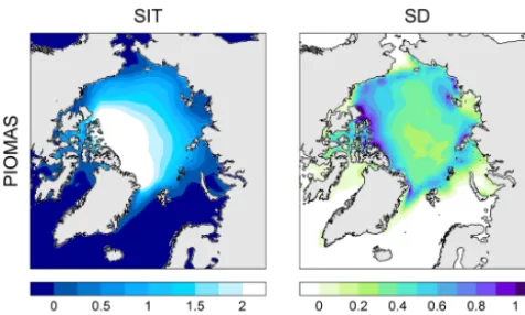
Figure 1. September 1979–2014 mean SIT and standard deviation
(SD) from the PIOMAS reanalysis. SD is calculated after removing the linear trend.
1.5 m, which is reasonable when compared to Haas and How-ell (2015) who measured ice along the Northwest Passage in May 2011 and April 2015 using airborne electromagnetic induction soundings, and to Tilling et al. (2015) who used CryoSat-2 for October and November 2010–2014. North of Greenland SIT exceeds 3.5 m, which is again comparable to CryoSat-2 for October and November 2010–2014 and is be-tween 0 and 1 m along the north Russian coast. The SIT is most variable around the edge of the ice pack and especially near land. An effective BC should ensure that the simulations replicate these patterns of mean SIT and SD over this recent period.
2.2 Global climate models
This paper utilises a subset of six GCMs from CMIP5. Since a large part of this work assesses SIT variability, it is neces-sary for each GCM to have multiple ensemble simulations in the historical period and for each of the representative con-centration pathways (RCPs) 2.6, 4.5, and 8.5 for future sce-narios (Van Vuuren et al., 2011). In addition, the GCM mean spring thickness must fall within the 10th and 90th percentile of PIOMAS (Stroeve et al., 2014), have a reasonable spatial resolution, and a somewhat resolved Canadian Archipelago. A consistent spatial distribution of land is needed for realis-tic and spatially complete multi-model means. The six GCMs that comprise this CMIP5 subset are listed in Table 1.
For the CMIP5 subset the historical simulations are used for the period 1979–2005. In most of the analysis for the pe-riod post-2005, the RCP8.5 scenario is used, which ramps up the amount of greenhouse gases to have a cumulative ef-fect of increasing the direct radiative forcing by 8.5 W m−2 (approximately 1370 ppm CO2equivalent) by 2100 (Van Vu-uren et al., 2011). The impact of other scenarios is com-pared later in the analysis. Figure 2 shows the 1979–2014 ensemble-mean September SIT for the CMIP5 subset, high-lighting the considerable differences between the model
sim-Figure 2. Mean September SIT for each of the six GCMs
consid-ered, averaged over the period 1979–2014.
ulations, and indicating that model bias is likely to be the dominant uncertainty in near-term projections.
The aim of the SIT BC outlined in this paper is to cor-rect the mean and variance in the CMIP5 subset shown in Fig. 2 to the PIOMAS statistics. Although this should im-prove short-term predictions, a caveat to this approach is that PIOMAS only yields one realisation of the past (see Lindsay et al. (2014) for discussion of PIOMAS forced with alternative atmospheric forcings). We have to assume that the relatively short period over which we have observations (36 years) captures a representative sample of the behaviour we expect from the climate system. In the short term, this is probably a reasonable assumption, as the GCMs will not have evolved far from their corrected state of the recent past; this assumption is explored further in Sect. 4.
3 Bias correction methodology
Table 1. List of models used: the CMIP5 subset and observations.
Institution Model name Ensemble
membersa Commonwealth Scientific and
Industrial Research Organisa-tion (CSIRO)
CSIRO Mark version 3.6.0: CSIRO-Mk3.6.0 (Rotstayn et al., 2012)
10
Met Office Hadley Centre Hadley Centre Global Environment Model version 2-Earth System: HadGEM2-ES (The HadGEM2 Devel-opment Team et al., 2011)
4
National Center for Atmospheric Research
Community Climate System Model, version 4: CCSM4 (Gent et al., 2011)
6
National Center for Atmospheric Research
Community Earth System Model, Community Atmo-sphere Model, version 5: CESM1-CAM (Meehl et al., 2013)
3
Model for Interdisciplinary Re-search on Climate (MIROC)
MIROC version 5: MIROC5 (Watanabe et al., 2010) 3
Max Plank Institute for Meteo-rology (MPI)
MPI Earth System Model, low resolution: MPI-ESM-LR (Jungclaus et al., 2006)
3
Applied Physics Laboratory (University of Washington)
Pan-Arctic Ice–Ocean Modelling and Assimilation Sys-tem: PIOMASb(Zhang and Rothrock, 2003)
1
amulti-model statistics are calculated (Sect. 4.3 onwards) using the first three ensemble members. bused as observations.
Figure 3. Performance of different SIT BCs for one particular month at a hypothetical grid point in a “toy” model. Mean, SD (detrended), and
trend legend statistics are calculated over the observation period (1979–2014). “Ice-free” is defined as the first occurrence of any ensemble member below 0.15 m. The ice-free ensemble range is shown; i.e. the year of the first ensemble member to be ice-free to the last ensemble member to be ice-free. The black line represents “observations”; the blue and red lines represent high and low ice models respectively. The thin coloured lines represent ensemble members, and the thick lines represent the ensemble mean.
this including Kay et al. (2011), Day et al. (2012), Notz and Marotzke (2012), Stroeve et al. (2012), Notz (2015), Swart et al. (2015) and Zhang (2015). We are also cautious of
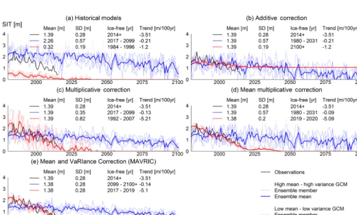
To test the performance of different possible BC methods, a toy model was used as proxy ensemble time series (repre-senting SIT at a single grid point for the same month each year for the period 1979–2100). The time series are shown in Fig. 3a for a high-mean–high-variance model (blue) and a low-mean–low-variance model (red), where the black line shows the “truth” (observations with one realisation over the historical period only). The time series were all produced using a first-order auto-regressive (with an AR(1) parame-ter of 0.3 chosen to be representative of CMIP5 SIT auto-correlation) model imposed on a declining linear trend with negative numbers reset to zero. Each model has five sepa-rate model ensemble members (thin coloured lines); the thick lines represent the ensemble means. The statistics in all the legends are calculated over the observation window (1979– 2014). “Ice-free” in Fig. 3 is here defined as the first occur-rence of an ensemble member below 0.15 m. Shown is the ice-free ensemble range, i.e. the year of the first ensemble member to be free to the last ensemble member to be ice-free. A successful BC method should transform the individ-ual ensemble members (thin red and blue lines) to match the mean and variance of the observations (black line), produc-ing matched statistics. We test various approaches for such a bias correction. The mathematical notation for the following equations is in Table 2.
3.1 Additive correction
A basic additive correction, which has previously been used for temperature projections, is shown in Fig. 3b. This ap-proach simply corrects the time mean by subtracting the dif-ference between the historical model ensemble-mean time mean, hMhi, and observation time mean,Oh, from each of the model ensemble members,M.
Additive corrected thickness=M− hMhi −Oh (1) However, as the low ice model is adjusted up by the ad-dition of a constant, it equilibrates at a positive value in the future rather than zero. Likewise the high ice model equili-brates at negative values. Neither of these properties are sen-sible.
This study makes use of multiple ensemble members from the same model, raising the question of how to treat ensemble member statistics when calculating a particular GCM’s bias. For calculating the mean SIT, each GCM’s ensemble mean is used because it is the GCM’s mean bias that we wish to cor-rect. This is important because a particular ensemble mem-ber’s deviation from the ensemble mean is retained; it allows an individual ensemble member’s time mean to be different to the observations over the historical period, but not the en-semble mean. The treatment of enen-semble members for the SD calculation is described in Sect. 3.4.
Table 2. Notation key.
Notation Description
M Model
Oh Observations
xh xover the historical period (1979–2014) x Time mean ofxover historical period
hxi Ensemble mean ofx e
x Running time mean (11 years) ofx
ˆ
x Temporally detrendedxover the historical period
σ Standard deviation
3.2 Multiplicative correction
If a multiplicative correction is used (Fig. 3c), where the ratio of the observed time mean and model ensemble-mean time mean,Oh/hMhi, is multiplied as a factor to the model ensem-ble members,M, then the corrected thickness is as follows.
Multiplicative corrected thickness=M Oh
hMhi
(2)
Multiplicative methods effectively preserve the future zero ice year, which is potentially an important value for a wide range of stakeholders. However, when applied as above this approach has the undesired effect of distorting the variances by the same factor as the mean correction, as visible in Fig. 3c.
3.3 Mean multiplicative correction
To avoid altering the variances, the mean multiplicative cor-rection can be introduced (Fig. 3d), where the multiplicative mean correction,Oh/hMhi, is applied only to the 11-year-centred running-mean ensemble mean, hMei. This corrects the model mean evolution without corrupting the sub-decadal variance ashMeiis smoothed. The model anomalies for each ensemble member,M− hMei, are then added back to the cor-rected mean evolution.
Mean multiplicative corrected thickness = M− hMei
+ hMei
Oh
hMhi
(3)
3.4 Mean and variance correction
The GCMs from CMIP5 show a large range in SIT variance, and the magnitude of these variations is a significant factor determining when regions of the Arctic may first become accessible (when one ensemble member may first become ice-free). Therefore a variance correction is incorporated into Eq. (3) by taking the ratio of the temporal standard deviation of the detrended observations,σ
c
Oh, to the square root of the ensemble mean of the variance of the detrended model en-sembles,hσMc
hi(detrended mean ensemble SD), over the his-torical period. The detrending in the models is calculated us-ing each model’s ensemble mean linear trend. This has some similarities to the approach of Ho et al. (2011) in application to temperature projections for Europe. See also Appendix A for some further discussion of the choices made.
To incorporate the variance correction, the mean multi-plicative correction (Eq. 3) is first de-trended, the variance correction applied, and the trend re-applied. This creates the Mean And VaRIance Correction (MAVRIC), shown in Eq. (4).
MAVRIC= M− hMei σOch
hσMc
hi + hMei
Oh
hMhi
(4) Figure 3e shows the MAVRIC does a near-perfect job of correcting both the mean and variance to the observed statis-tics while still retaining the individual ensemble members’ own climate fluctuations, but being fractionally scaled by the variance ratio.
Comparing the ensemble range in projected ice-free date between the correction methods, it is apparent that although the shapes of time series have qualitatively changed, this does not always result in a different range in projected ice-free date. For example the difference evident on comparing the high-mean–high-variance GCM (blue) between (a) to (c) and (b) to (d) is partly coincidence and partly due to how the four correction methods shown manipulate the time series. The MAVRIC method (e) results in a unique set of ice-free dates. This is an important attribute that the MAVRIC method dis-plays, as the ice-free date is of vital importance to stakehold-ers in the Arctic and more basic methods of bias correction fail to appropriately adjust this parameter.
4 Bias corrected sea ice thickness projections
Figure 3e illustrates that the MAVRIC successfully corrects the mean and variance in a toy model environment. Before proceeding to investigate the impact of the MAVRIC on SIT projections, it is prudent to test whether the MAVRIC can improve GCM performance by validating with PIOMAS. We use CSIRO-Mk3.6.0 (CSIRO) as the GCM to test. The ice in CSIRO generally has too much areal coverage and too little variability and is a CMIP5 outlier model with regards to SIT (Stroeve et al., 2014). However, CSIRO benefits from hav-ing 10 ensemble members, increashav-ing the robustness of the
statistics. For these two reasons, it is considered a thorough test of the MAVRIC’s performance within a real GCM.
The test uses a data denial method where we train the MAVRIC on a subset of PIOMAS observations, 1979–1999, termed the “calibration window”. From this we examine how the MAVRIC predicts the observations for 2000–2014, termed the “validation window”. A limitation of this method is the length of observations: the period over which the MAVRIC calibration takes place must be long enough to capture a robust measure of the observed statistics. The vali-dation period must also be long enough to be able to draw robust conclusions. It is not clear whether either the 21-year calibration or the 15-21-year validation windows are long enough for robust method calibration and results verification, but we are limited by the data available. An additional lim-itation to this method is that the calibration and validation periods are very close to each other.
Figure 4 shows the performance of the MAVRIC at three grid points for September. The raw CSIRO ensembles (grey) are bias-corrected via the MAVRIC using the PIOMAS ob-servations (black) over the calibration window, producing the MAVRIC corrected ensembles (green) for the validation window. If the MAVRIC can produce plausible predictions, the characteristics of PIOMAS should be indistinguishable from individual corrected ensemble members in the valida-tion window. It is clear from the validavalida-tion bean plots (right), that the distribution from the corrected ensembles resembles PIOMAS much more closely than the raw distribution, e.g. non-zero probability of zero ice. We do not expect the distri-bution from PIOMAS to match the corrected distridistri-bution per-fectly as PIOMAS only has one realisation (15 data points) while CSIRO has 10 realisations. We can tentatively accept that this test demonstrates the validity of the MAVRIC ap-proach.
In the following sections the MAVRIC is applied to the CMIP5 subset of six GCMs used in this study (Table 1). PI-OMAS estimates of Arctic SIT are available from 1979 to 2014. This 36-year window is the period over which statistics are calculated in the observations, and in the CMIP5 subset (using historical runs for 1979–2005 and RCP8.5 for 2006– 2014). Each model, month, and grid point has its own spe-cific correction which is applied to all years (1979–2100). However, separate ensemble members from the same GCM are treated with the same correction, as we wish to correct the model bias and retain the ensemble spread. Results are shown for September, initially only for CSIRO and later for all six models combined to form the CMIP5 subset used for this study.
4.1 Temporal perspective example
PI-Figure 4. September SIT at three grid point locations in the Arctic, from PIOMAS (black) and CSIRO-Mk3.6.0 historical (1979–2005) and
RCP8.5 (2006–2014) raw output (grey) and post-MAVRIC (green). The raw CSIRO ensembles (grey) are bias-corrected via the MAVRIC using the PIOMAS observations (black) over the calibration window, producing the MAVRIC ensembles (green) for the validation window. Bean plots (right) show the distribution of the SIT for the validation period. The small horizontal lines show every SIT value, the frequency of which is illustrated by the width of the shaded region. The thick horizontal line depicts the mean.
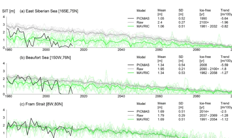
Figure 5. September SIT at three grid point locations in the Arctic, from PIOMAS (black) and CSIRO-Mk3.6.0 historical (1979–2005) and
RCP8.5 (2006–2100) raw output (grey) and post-MAVRIC (green). Thin lines show individual ensemble members; thick lines show the ensemble means. Mean, SD, and trend legend statistics are calculated over the period of observations (1979–2014). The SD is the detrended mean ensemble SD. The range of the first occurrence of the first and last ensemble member below 0.15 m is considered to be ice-free.
OMAS (Fig. 5a). The correction therefore reduces the mean SIT whilst increasing the variance. This brings forward the range of first year ice-free conditions (the first occurrence in each ensemble member of a SIT below 0.15 m) from after
simi-Figure 6. CSIRO-Mk3.6.0 and HadGEM2-ES, September 1979–
2014 ensemble mean SIT and SD (detrended). The raw columns are the model solutions as found in the CMIP5 archive. The corrected columns show the distribution after the MAVRIC has been applied. PIOMAS SIT fields are shown in Fig. 1.
lar SIT, requiring only a small mean adjustment; however CSIRO requires a big increase in variance. The MAVRIC moves the first possible ice-free date about 30 years earlier and increases the ensemble range from 32 to 63 years. It is worth noting that the dominant cause of this shift to an ear-lier ice-free date at this location is due to the variance cor-rection term in the MAVRIC rather than the mean corcor-rection term. This highlights the importance of correcting the vari-ance in addition to the mean. Figure 5 demonstrates that the MAVRIC can lead to simulations that look significantly more like reality in the historical period and have an impact on re-gional ice-free projections.
4.2 Historical spatial perspective
In addition to examining the MAVRIC in a temporal sense, it is important to evaluate the results spatially to see where the MAVRIC is having the most effect and if it works at all lo-cations. Figures 2 and 6 show that the mean September SIT distribution is very different in HadGEM2-ES and CSIRO. After the MAVRIC has been applied, the mean SIT fields are almost identical for the historical period (Fig. 6). It is im-portant to note there are still differences when considering individual years and ensemble members i.e. the year-to-year variability and ensemble spread is preserved (although ad-justed by the MAVRIC).
Figure 6 also shows the SD before and after the MAVRIC. The SD shown is the detrended mean ensemble SD as before. CSIRO has a variability that is too low in the majority of locations, although it correctly places the maximum SD near the edges of the ice pack similarly to PIOMAS. HadGEM2-ES exhibits about the same magnitude of variability as the observations but the variability is too high in the centre of the ice pack and too low at the edges. After the correction, the SD fields in both GCMs now look more similar to each other, with the highest variability located at the edge of the
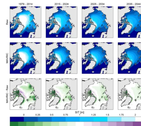
Figure 7. September multi-model ensemble mean (three members
from each model) mean SIT from the CMIP5 subset, using the raw data (top row) and post-MAVRIC (middle row). The bottom row shows (MAVRIC – raw); hence green areas are where MAVRIC has reduced SIT and purple areas are where MAVRIC has increased SIT.
ice pack and at coastal locations. They are now also both similar to the estimate from PIOMAS (Fig. 1).
4.3 CMIP5 subset multi-model sea ice thickness projections
The bias-corrected SIT from each GCM can be brought to-gether to form the multi-model mean CMIP5 subset, com-puted using three ensemble members (the maximum avail-able across all models) from each of the six GCMs for the historical and future decadal periods (Fig. 7). It is remark-able how the raw multi-model mean product for the historical period is not too different from PIOMAS in Fig. 1, showing that the location and magnitude of model biases cancel out to a considerable degree, at least with this subset of models. Given this result it is not so surprising that the raw and cor-rected fields are fairly similar for the future projections also. Nevertheless, even in this multi-model multi-ensemble framework the MAVRIC is still making some discernible dif-ferences. These differences are most apparent in the Cana-dian Archipelago and the Russian Arctic seas, where the cor-rection leads to a reduction in SIT of approximately 1 m in both regions. Both the raw and bias-corrected fields predict a SIT loss of about 0.25 m per decade.
ab-Figure 8. September 2015–2024 sources of SIT uncertainty from
the CMIP5 subset (SD of the detrended SIT). The multi-model en-semble mean (three members from each) is shown when comparing raw output (top row) and post-MAVRIC (bottom row).
solute value of SIT, do not yet account for such factors and will need to be reassessed.
4.4 Sources of uncertainty in projections of sea ice thickness
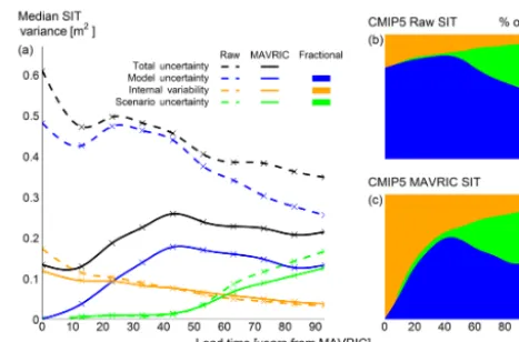
The uncertainty in climate projections can be partitioned into three distinct sources: (1) model uncertainty: for the same radiative forcing, different models simulate different mean distributions and temporal changes; (2) internal variability: the natural fluctuations of the climate present with or with-out any anthropogenic induced changes to radiative forcing; (3) scenario uncertainty: uncertainty in future radiative forc-ing resultforc-ing from unknown future emissions. Hawkins and Sutton (2009, 2011) assessed these sources of uncertainty in global and regional temperature and precipitation projec-tions, and here we quantify the sources of uncertainty in SIT, utilising the CMIP5 subset multi-model ensemble. Crucially we use the absolute values of SIT rather than considering anomalies as is often done for other climate variables. The methodology for partitioning these sources of uncertainty is detailed in Appendix B. An additional source of uncer-tainty that we neglect here is the PIOMAS calibration un-certainty emerging from the choice of atmospheric reanaly-sis and model tuning. This could be assessed by sampling the different versions of the PIOMAS reanalysis described in Lindsay et al. (2014). They find the different versions are broadly similar and can be accounted for by appropriate tun-ing of the ice model component. This bias in PIOMAS itself will introduce systematic biases to the MAVRIC projections. This bias is not a flaw in MAVRIC however but a limitation intrinsic to the observational data set one is correcting to.
The MAVRIC method outlined in this study acts to elim-inate the model bias in the MAVRIC calibration period (1979–2014). After this period the model uncertainty grows due to the GCM’s differing responses to changes in external forcing. The sources of uncertainty for SIT for the decade
Figure 9. The evolution of the sources of September SIT
un-certainty in the CMIP5 sub-set with lead time. Year zero is the MAVRIC window mid-point (1997) and the emission scenarios (RCPs) start in 2006. Panel (a) shows the change in magnitude of the different sources of uncertainty. The uncertainty shown is the median SIT variance and hence the lines scale additively. The dashed lines are for the raw model output and solid lines are for post-MAVRIC. Contributions of model uncertainty, internal vari-ability, and scenario uncertainty as a fraction of total uncertainty are shown for the raw output (b) and post-MAVRIC (c).
2015–2024, immediately following the MAVRIC calibration period, are shown in Fig. 8. The total uncertainty in the corrected CMIP5 subset is strikingly lower than in the raw CMIP5 subset. Closer analysis reveals that this is due to the substantial reduction in model uncertainty owing to the MAVRIC. The other sources of uncertainty do not change as much.
The temporal evolution of these sources of uncertainty is shown in Fig. 9a by taking the median variance from each of the panels in Fig. 8 for this and other periods. There are three competing factors for how the uncertainty will change with time. First, the SIT is decreasing, and this will reduce the uncertainty as the range of values of which the SIT can occupy shrinks. Second, the separate GCMs’ simulated SIT responses due to external forcing will differ from each other, causing GCMs to drift apart over time. Thirdly, sea ice at the grid point scale becomes more mobile and vulnerable to external factors as it thins. This will increase variability, ini-tially at least (Sou and Flato, 2009). All of these factors are involved in the evolution of the uncertainties.
subsequently diverge because of differing responses to the changes in external forcing. Later the corrected model un-certainty reduces as the mean SIT decreases towards zero.
The total uncertainty is the sum of model uncertainty, in-ternal variability, and scenario uncertainty (see Appendix B for more details). The other panels in Fig. 9 illustrate the rel-ative importance of these sources of uncertainty in terms of the percentage total variance explained, for the raw data, and after the MAVRIC.
Figure 9b illustrates that in the raw projections, model uncertainty remains the dominant (> 50 %) source of uncer-tainty until at least 2100, whereas it only becomes dominant for a few decades mid-century after the MAVRIC (Fig. 9c). The absolute magnitude of internal variability, and its contri-bution to the total uncertainty, decreases with time because SIT also decreases with time. In the corrected projections, the internal variability is the major contributor to the total uncertainty for the first 25 years, compared to a maximum contribution of only 26 % in the raw projections. This high-lights the importance of correcting the variance to realistic magnitudes and also the key role of natural variations in pre-dicting the near-future evolution of sea ice. The scenario un-certainty accounts for less than 10 % of the total unun-certainty for the first 50+ years. Additional analysis metrics on the im-provement that the MAVRIC method affords can be found in Appendix C.
Although we have demonstrated here that the MAVRIC method reduces the model uncertainty as seen by the reduc-tion in spread of projected SIT with our selecreduc-tion of GCMs, we acknowledge that this may not necessarily correspond to a reduction in uncertainty in the real world.
4.5 Reduced spread in timing of ice-free conditions By reducing the model spread the range of possible out-comes has been reduced, this potentially leads to greater con-fidence in SIT projections. Figure 10 shows the raw and cor-rected CMIP5 subset SIV* projections until 2100 using the 18 multi-model ensemble members in each scenario as be-fore (* calculated here does not consider spatial SIC as it is not bias-corrected). To find a representative SIC for the SIV* calculation we use the September SIC in CCSM4 RCP8.5 and find a mean (of the non-zero grid cells) SIC of approxi-mately 50 % for 2006–2100.
The thick coloured lines show the multi-model scenario mean and the coloured regions represent the 16–84 % (equiv-alent to 1σ around the mean of a Gaussian distribution) of the ensemble members. To account for the large range in SIT at any particular time in the CMIP5 subset, we use a method similar to that of Massonnet et al. (2012) to calculate first ice-free conditions. We postulate that SIV for ice-ice-free conditions is 1×10³km3, which is in agreement with previous studies calculating first ice-free dates (e.g. Massonnet et al. (2012) and Overland and Wang, 2013), and is equivalent to 1 m thick ice for an ice extent of 106km2.
Figure 10. CMIP5 subset sea ice volume (SIV*) projections and
first ice-free conditions. Panels (a, b) show the projected SIV* from all six models (18 ensemble members total) in both the raw and corrected GCMs (11-year running mean), and shaded regions are the 16th–84th percentiles. Panel (c) shows the number of ensemble members having passed the ice-free threshold. Panel (d) shows the statistics of (c), with the whiskers representing the range (1st and 18th ensemble member ice-free), the box capturing the 16th–84th percentiles, and the bold line showing the median (9th ensemble member). Ice-free is defined as the first year the pan-Arctic SIV* dips below 1×10³km3 for a particular ensemble member. *Vol-ume (SIV*) is calculated using a constant 50 % SIC throughout.
The MAVRIC reduces the total SIV, but the relative mag-nitude of this reduction decreases as SIV declines. The 16– 84 % range has also been vastly reduced, particularly for the near future. For example, in 2025 the MAVRIC has reduced the 16–84 % range from 6×10³km3to 2.5×10³km3. It is this reduction in the plausible range of SIV that leads to po-tential increased confidence in projections of SIT and SIV. To assess when the Arctic will first display ice-free condi-tions, we focus on RCP8.5, the most realistic scenario from the last 10 years (Fuss et al., 2014). The cumulative number of ensemble members having satisfied the ice-free criterion as a function of time is shown in Fig. 10c. If the range in this parameter has reduced, this will be shown by the gradient of the line increasing post-MAVRIC, and this is clearly seen. Figure 10d further illustrates the spread reduction with box plots, where the internal line represents the median (9th) en-semble member to go ice-free. This occurs in 2052 with the MAVRIC, 9 years earlier than before. The box represents 16– 84 % of the ensemble members. This range has been reduced by about 20 years; dates after 2085 can now be eliminated.
MAVRIC are in good agreement by the end of the century, with projected ice-free dates around 2090.
5 Summary and discussion 5.1 Summary
This study has developed a bias correction methodology for simulations of sea ice thickness (SIT). By constraining CMIP5 simulations with the PIOMAS reanalysis we have demonstrated the following.
– GCMs simulate a wide range of SIT in the histori-cal period and exhibit various spatial and temporal bi-ases when compared with the PIOMAS reanalysis. This model uncertainty (or bias) is the dominant source of uncertainty in CMIP5 future climate projections of SIT. – The Mean And VaRIance Correction (MAVRIC) tech-nique outlined in this paper significantly reduces the to-tal uncertainty in future projections of SIT as far as 2100 by reducing model uncertainty. Correcting both mean and variance of models is found to be critical for im-proving the robustness of the projections.
– The MAVRIC results in internal variability being the dominant source of uncertainty until 2022, and model uncertainty is dominant thereafter. From the mid-century onwards, scenario uncertainty becomes increas-ingly important and as influential as model uncertainty by 2100.
– The MAVRIC results in projected September ice-free conditions in the Arctic under RCP8.5 occurring up to 10 years earlier (2050s) than without the correction, and with a considerably narrower range, e.g. excluding post-2085 dates.
5.2 Discussion
Without the MAVRIC, the true magnitude of the internal variability and scenario uncertainty in projections of SIT is concealed by the dominant model uncertainty. This demon-strates that time invested in running many ensemble members to sample internal variability in SIT may be more beneficial than running many future emission scenarios for near-term projections. These findings implicate that there is room for improvement in GCMs at least for 50-year projections where the scenario differences are negligible. However, for projec-tions at the end of the century, the scenarios become more important.
The MAVRIC bias correction technique developed in this study results in a significant improvement in model simula-tions of SIT with respect to observasimula-tions. In future projec-tions, the MAVRIC results in a substantial reduction in the range of SIT, potentially leading to increased confidence in climate projections. As absolute values of SIT are utilised, this reduction in spread potentially has important implica-tions for stakeholder sectors operating in Arctic waters such as the shipping industry. The application of the bias correc-tion results in a 60 % reduccorrec-tion in the likely range (16–84 %) of sea ice volume in September 2025.
There are a number of caveats to these findings. No at-tempt is made to constrain the trend in the GCMs. This would be difficult because of the short timescale over which obser-vations are available, raising serious questions about the ro-bustness of calculated historical trends. However future stud-ies could consider this further and assess the feasibility of a trend correction to GCMs. In addition, it is important to recognise that PIOMAS, used here as observations, will also have errors. It would be possible to reduce the multiplicative weightings in Eq. (4) to reflect some uncertainty in the his-torical data. Other temporally and spatially complete sea ice reanalyses could also be used in future to address this issue.
The simulations tend to show an increase in variance as the sea ice thins, before subsequently declining as the thickness approaches zero (Goosse et al., 2009). Blanchard-Wrigglesworth and Bitz (2014) assessed the relationship of this mean state-dependent variance in 19 GCMs, including five of the six used in this study, in addition to PIOMAS. They find a relationship between mean thickness variabil-ity and mean thickness in models; i.e. models with thicker SIT depict more variable SIT. In the 19 GCMs assessed, PI-OMAS sits on the trend line for the correlation between mean thickness variability and mean thickness. However, in the de-veloped MAVRIC, the change in variance is decoupled from the applied change to the mean state. This aspect could be further developed, but only by making additional assump-tions about future changes in SIT variability.
Appendix A: Supplementary MAVRIC methodology details
For model biases to be calculated a common grid needed to be used; hence all MAVRIC calculations took place on the CMIP5 model’s native grid. This means that PIOMAS was converted to the CMIP5 model grid for each GCM’s bias calculations. This choice was made as it only involves in-terpolating one of the two fields each time and generally it is PIOMAS that has the higher resolution. The BC shown in Eq. (4) contains two terms for the representation of the variance in both observationsσOc
h and modelsσMch. Over the 36-year period of observations the magnitude of the ice loss trend can be significant. To accurately calculate variances this externally forced trend should first be removed to leave the variance due to internal variability. Here a choice needs to be made about how best to remove the externally forced trend. For the PIOMAS observations we choose to linearly detrend the monthly data. A smoothed detrending was con-sidered, however this might remove longer timescale vari-ability which is undesirable. Using similar reasoning it is possible that the linear detrending removes some variabil-ity on the multi-decadal timescale. This is assumed to be significantly less than variability on smaller timescales, and much of the trend is attributed to be externally forced over the 36 years, hence should not be included as internal vari-ability. The performance of a smoothed detrend was tested in a theoretical framework and resulted in a 10 % loss of ac-curacy in the standard deviation correction due to describing variance as trend.
The calculation of variance in the models is more compli-cated due to the fact that there is more than one realisation. It is obvious that the required variance should be calculated from the individual ensemble members rather than the semble mean. The variance should be calculated in each en-semble member and then the mean taken. There is another choice to make, i.e. whether each ensemble member should be detrended with its own trend, or whether the ensemble mean trend should be used. We propose that the ensemble mean trend should be used as this is the models’ response to the changes in forcings. The model detrended ensemble mean standard deviation,σMc
h, was calculated by calculating the detrended ensemble variances, then taking the square root of their mean.
The running mean for the future model correction term hMei is calculated over an 11-year period of the ensemble mean; this window hence starts at 1975 for the historical calculations. The chosen period must be long enough to ad-equately smooth the time series, whilst still being able to capture variations in the sea ice decline trend. This was also tested and found to outperform a 21-year period.
Appendix B: Partitioning sources of uncertainty
The sources of uncertainty in Sect. 4.4, Figs. 8 and 9, are calculated for each decadal period (2005–2014, 2015– 2024, etc.) separately as follows. Three ensemble mem-bers from each of the six GCMs are utilised for three dif-ferent emission scenarios (RCP2.6, 4.5, and 8.5). This re-sults in each decade having 6 (GCMs)×3 (ensemble mem-bers)×3 (scenarios)×10 (years)=540 (fields).
– The total uncertainty is the variance calculated across all 540 fields.
– The internal variability is calculated similarly to the total variability except instead of the absolute values, the anomalies from the models’ decadal-mean ensem-ble mean for each scenario are used.
– To calculate the model uncertainty, each of the six mod-els’ decadal-mean ensemble mean is calculated, result-ing in six fields. The variance is then calculated across these six fields, and repeated for all three scenarios sep-arately (to eliminate differential model dependent re-sponses to the different emission scenarios). The model uncertainty is the square root of the mean of these three fields.
– The scenario uncertainty is calculated in a similar way. For each model, each of the three scenarios decadal-mean ensemble decadal-means are calculated resulting in three (scenario-dependent) decadal-mean ensemble means for each of the six models. The variance is then calcu-lated through these three scenario mean fields for each of the six models, resulting in six fields of the variance in each model. The square root of the mean of the six models’ scenario uncertainty is the scenario uncertainty. To create Fig. 8b and c it is assumed that the total variance (total uncertainty,T2)is the sum of the variance due to model uncertainty (M2), internal variability (I2), and scenario un-certainty (S2), formally:
T2=M2+I2+S2. (B1)
Appendix C: Additional MAVRIC performance analysis To highlight whether the estimated uncertainties are reliable, we examine the errors in the projections when considering one member as “truth”. As all ensemble members are con-strained by PIOMAS, one individual ensemble member out of sample should fall within the distribution of the remain-ing ensemble members. This principle should hold true for all ensemble members out of sample in turn.
The root-mean-square error (RMSE) is calculated using Eq. (C1):
RMSE= v u u t
1 18
18 X
n=1
En−E15 2
, (C1)
whereEnis the ensemble member between 1 and 18;E15 is the mean of the 15 ensemble members from the models of whichEnis not a member.
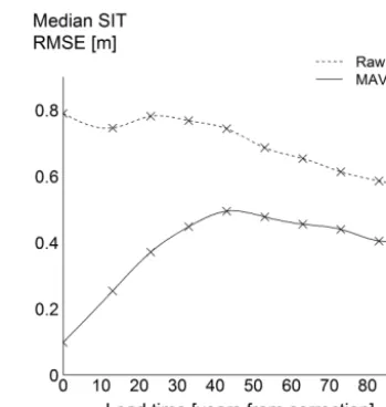
Figure C1 shows the advantage of the MAVRIC method in this out of sample RMSE test. A decreasing RMSE means that the models are initially biased though are converging to a common value (as we expect in this case as the models trend towards being ice-free). An increasing RMSE means that the models are diverging as they have different ice loss trends.
The MAVRIC ensemble trained on every individual en-semble member within MAVRIC results in an RMSE of 0.1 m initially and up to a maximum RMSE of 0.5 m. The fact that the raw RMSE decreases (as opposed to increases) high-lights that the models have biases. The 0.1 m in the MAVRIC RMSE indicates that initially the MAVRIC ensemble mem-bers differ only in internal variability. The RMSE then grows due to differing ice loss trends, which is expected as there is no attempt to correct the trends in this study.
To find the dispersion of the MAVRIC multi-model en-semble we repeat this style of experiment with the standard error (SE) metric, using Eq. (C2):
SE=En−E15
σ15
, (C2)
whereEnis the ensemble member between 1 and 18;E15 is the mean of the 15 ensemble members from the models of whichEnis not a member.σ15is the standard deviation of the 15 ensemble members of whichEnis not a member. This is repeated for all 18 ensemble members, giving 18 SEs of how different each ensemble member is to the rest of the multi-model ensemble set. The SD across these 18 SEs is the dis-persion of the multi-model ensemble. A perfectly dispersed ensemble set will have a dispersion of 1. Numbers less than 1 mean the ensemble set is under-dispersed and hence predic-tions/projections from that set will be under-confident as the SD is too large. Values greater than 1 indicate that the system is over-dispersive and hence over-confident.
The results of the dispersion calculation are shown in Fig. C2. The MAVRIC ensemble is approximately 15– 30 % over-dispersed for lead times of up to 60 years. This
Figure C1. Multi-model ensemble out of sample September median
SIT RMSE.
Figure C2. Multi-model ensemble out of sample September median
SIT dispersion.
Author contributions. N. Melia, K. Haines, and E. Hawkins
de-signed the methodology and experiments. N. Melia developed the code, and performed the experiments. N. Melia, K. Haines, and E. Hawkins wrote the manuscript.
Acknowledgements. We thank Steffen Tietsche for the conversion
of the PIOMAS data, and Daniel Feltham and Ellie Highwood for their comments on a pre-submission draft. We thank referees Gre-gory Flato and Francois Massonnet for their quick responses and thorough and constructive reviews. We thank Robert Darby and the University of Reading Research Data Archive for facilitating the hosting of the MAVRIC data set. All statistical analyses and figures were accomplished using the R language and environment for statistical computing and graphics. For more information, see http://www.r-project.org/.
N. Melia and E. Hawkins are funded by the APPOSITE project (grant NE/I029447/1), funded by the UK Natural Environment Research Council as part of the Arctic Research Programme. E. Hawkins is also funded by NERC Fellowship. K. Haines is partly funded by the National Centre for Earth Observation NCEO. Edited by: J. Stroeve
References
Blanchard-Wrigglesworth, E. and Bitz, C. M.: Characteristics of Arctic Sea-Ice Thickness Variability in GCMs, J. Climate, 27, 8244–8258, doi:10.1175/Jcli-D-14-00345.1, 2014.
Boe, J., Hall, A., and Qu, X.: September sea-ice cover in the Arc-tic Ocean projected to vanish by 2100, Nat. Geosci, 2, 341–343, doi:10.1038/ngeo467, 2009.
Christensen, J. H., Boberg, F., Christensen, O. B., and Lucas-Picher, P.: On the need for bias correction of regional climate change projections of temperature and precipitation, Geophys. Res. Lett., 35, L20709, doi:10.1029/2008gl035694, 2008. Day, J. J., Hargreaves, J. C., Annan, J. D., and Abe-Ouchi, A.:
Sources of multi-decadal variability in Arctic sea ice extent, Env-iron. Res. Lett., 7, 034011, doi:10.1088/1748-9326/7/3/034011, 2012.
Flato, G., Marotzke, J., Abiodun, B., Braconnot, P., Chou, S. C., Collins, W., Cox, P., Driouech, F., Emori, S., Eyring, V., Forest, C., Gleckler, P., Guilyardi, E., Jakob, C., Kattsov, V., Reason, C., and Rummukainen, M.: Evaluation of Climate Models, in: Cli-mate Change 2013: The Physical Science Basis. Contribution of Working Group I to the Fifth Assessment Report of the Inter-governmental Panel on Climate Change, edited by: Stocker, T. F., Qin, D., Plattner, G.-K., Tignor, M., Allen, S. K., Boschung, J., Nauels, A., Xia, Y., Bex, V., and Midgley, P. M., Cambridge University Press, Cambridge, UK and New York, NY, USA, 741– 866, 2013.
Francis, J. A. and Vavrus, S. J.: Evidence linking Arctic amplifica-tion to extreme weather in mid-latitudes, Geophys. Res. Lett., 39, L06801, doi:10.1029/2012gl051000, 2012.
Fuss, S., Canadell, J. G., Peters, G. P., Tavoni, M., Andrew, R. M., Ciais, P., Jackson, R. B., Jones, C. D., Kraxner, F., Nakicenovic, N., Le Quere, C., Raupach, M. R., Sharifi, A., Smith, P., and
Yamagata, Y.: Betting on negative emissions, Nat. Clim. Change, 4, 850–853, doi:10.1038/nclimate2392, 2014.
Gent, P. R., Danabasoglu, G., Donner, L. J., Holland, M. M., Hunke, E. C., Jayne, S. R., Lawrence, D. M., Neale, R. B., Rasch, P. J., and Vertenstein, M.: The community climate system model version 4, J. Climate, 24, 4973–4991, 2011.
Goosse, H., Arzel, O., Bitz, C. M., de Montety, A., and Van-coppenolle, M.: Increased variability of the Arctic summer ice extent in a warmer climate, Geophys. Res. Lett., 36, L23702, doi:10.1029/2009gl040546, 2009.
Haas, C. and Howell, S. E. L.: Ice thickness in the North-west Passage, Geophys. Res. Lett., 42, 7673–7680, doi:10.1002/2015gl065704, 2015.
Hawkins, E. and Sutton, R.: The Potential to Narrow Uncertainty in Regional Climate Predictions, B. Am. Meteorol. Soc., 90, 1095– 1107, doi:10.1175/2009bams2607.1, 2009.
Hawkins, E. and Sutton, R.: The potential to narrow uncertainty in projections of regional precipitation change, Clim. Dynam., 37, 407–418, doi:10.1007/s00382-010-0810-6, 2011.
Ho, C. K., Stephenson, D. B., Collins, M., Ferro, C. A. T., and Brown, S. J.: Calibration Strategies: A Source of Additional Un-certainty in Climate Change Projections, B. Am. Meteorol. Soc., 93, 21–26, doi:10.1175/2011bams3110.1, 2011.
Jungclaus, J., Keenlyside, N., Botzet, M., Haak, H., Luo, J.-J., Latif, M., Marotzke, J., Mikolajewicz, U., and Roeckner, E.: Ocean circulation and tropical variability in the coupled model ECHAM5/MPI-OM, J. Climate, 19, 3952–3972, 2006.
Kay, J. E., Holland, M. M., and Jahn, A.: Inter-annual to multi-decadal Arctic sea ice extent trends in a warming world, Geo-phys. Res. Lett., 38, L15708, doi:10.1029/2011gl048008, 2011. Kwok, R., Cunningham, G. F., Wensnahan, M., Rigor, I., Zwally, H.
J., and Yi, D.: Thinning and volume loss of the Arctic Ocean sea ice cover: 2003–2008, J. Geophys. Res.-Oceans, 114, C07005, doi:10.1029/2009jc005312, 2009.
Laxon, S. W., Giles, K. A., Ridout, A. L., Wingham, D. J., Willatt, R., Cullen, R., Kwok, R., Schweiger, A., Zhang, J., Haas, C., Hendricks, S., Krishfield, R., Kurtz, N., Farrell, S., and Davidson, M.: CryoSat-2 estimates of Arctic sea ice thickness and volume, Geophys. Res. Lett., 40, 732–737, doi:10.1002/Grl.50193, 2013. Lindsay, R., Wensnahan, M., Schweiger, A., and Zhang, J.: Eval-uation of Seven Different Atmospheric Reanalysis Products in the Arctic, J. Climate, 27, 2588–2606, doi:10.1175/jcli-d-13-00014.1, 2014.
Lindsay, R. W. and Zhang, J.: Assimilation of Ice Concentration in an Ice–Ocean Model, J. Atmos. Ocean. Tech., 23, L21502, doi:10.1029/2012gl053576, 2006.
Lindsay, R. W., Haas, C., Hendricks, S., Hunkeler, P., Kurtz, N., Paden, J., Panzer, B., Sonntag, J., Yungel, J., and Zhang, J.: Seasonal forecasts of Arctic sea ice initialized with ob-servations of ice thickness, Geophys. Res. Lett., 39, L21502, doi:10.1029/2012gl053576, 2012.
Mahlstein, I. and Knutti, R.: September Arctic sea ice predicted to disappear near 2◦C global warming above present, J. Geophys. Res.-Atmos., 117, D06104, doi:10.1029/2011jd016709, 2012. Massonnet, F., Fichefet, T., Goosse, H., Bitz, C. M.,
Meehl, G. A., Washington, W. M., Arblaster, J. M., Hu, A., Teng, H., Kay, J. E., Gettelman, A., Lawrence, D. M., Sanderson, B. M., and Strand, W. G.: Climate change projections in CESM1 (CAM5) compared to CCSM4, J. Climate, 26, 6287–6308, 2013. Melia, N.: Improved Arctic sea ice thickness projections using bias corrected CMIP5 simulations, University of Reading, Reading, UK, available at: http://dx.doi.org/10.17864/1947.9, last access: 22 October 2015.
Notz, D.: How well must climate models agree with observations?, Philos. T. Roy. Soc. A, 373, 2052, doi:10.1098/rsta.2014.0164, 2015.
Notz, D. and Marotzke, J.: Observations reveal external driver for Arctic sea-ice retreat, Geophys. Res. Lett., 39, L08502, doi:10.1029/2012gl051094, 2012.
Overland, J. E. and Wang, M.: When will the summer Arctic be nearly sea ice free?, Geophys. Res. Lett., 40, 2097–2101, doi:10.1002/grl.50316, 2013.
Rotstayn, L. D., Jeffrey, S. J., Collier, M. A., Dravitzki, S. M., Hirst, A. C., Syktus, J. I., and Wong, K. K.: Aerosol- and greenhouse gas-induced changes in summer rainfall and circulation in the Australasian region: a study using single-forcing climate simula-tions, Atmos. Chem. Phys., 12, 6377–6404, doi:10.5194/acp-12-6377-2012, 2012.
Schweiger, A., Lindsay, R., Zhang, J., Steele, M., Stern, H., and Kwok, R.: Uncertainty in modeled Arctic sea ice volume, J. Geo-phys. Res.-Oceans, 116, C00D06, doi:10.1029/2011jc007084, 2011.
Seneviratne, S. I., Nicholls, N., Easterling, D., Goodess, C. M., Kanae, S., Kossin, J., Luo, Y., Marengo, J., McInnes, K., and Rahimi, M.: Changes in climate extremes and their impacts on the natural physical environment, in: Managing the risks of ex-treme events and disasters to advance climate change adapta-tion, edited by: Field, C. B., Barros, V., Stocker, T. F., Qin, D., Dokken, D. J., Ebi, K. L., Mastrandrea, M. D., Mach, K. J., Plat-tner, G. K., K., A. S., Tignor, M., and M., M. P., A Special Re-port of Working Groups I and II of the Intergovernmental Panel on Climate Change (IPCC), Cambridge University Press, Cam-bridge, UK, and New York, NY, USA, 109–230, 2012.
Smith, L. C. and Stephenson, S. R.: New Trans-Arctic shipping routes navigable by midcentury, P. Natl. Acad. Sci. USA, 110, E1191–E1195, doi:10.1073/pnas.1214212110, 2013.
Sou, T. and Flato, G.: Sea Ice in the Canadian Arctic Archipelago: Modeling the Past (1950–2004) and the Future (2041–60), J. Cli-mate, 22, 2181–2198, doi:10.1175/2008jcli2335.1, 2009. Stephenson, S., Smith, L., Brigham, L., and Agnew, J.: Projected
21st-century changes to Arctic marine access, Clim. Change, 118, 885–899, doi:10.1007/s10584-012-0685-0, 2013.
Stroeve, J., Serreze, M., Holland, M., Kay, J., Malanik, J., and Bar-rett, A.: The Arctic’s rapidly shrinking sea ice cover: a research synthesis, Clim. Change, 110, 1005–1027, doi:10.1007/s10584-011-0101-1, 2012.
Stroeve, J., Barrett, A., Serreze, M., and Schweiger, A.: Using records from submarine, aircraft and satellites to evaluate climate model simulations of Arctic sea ice thickness, The Cryosphere, 8, 1839–1854, doi:10.5194/tc-8-1839-2014, 2014.
Swart, N. C., Fyfe, J. C., Hawkins, E., Kay, J. E., and Jahn, A.: In-fluence of internal variability on Arctic sea-ice trends, Nat. Clim. Change, 5, 86–89, doi:10.1038/nclimate2483, 2015.
Taylor, K. E., Stouffer, R. J., and Meehl, G. A.: An overview of CMIP5 and the experiment design, B. Am. Meteorol. Soc., 93, 485–498, doi:10.1175/Bams-D-11-00094.1, 2012.
The HadGEM2 Development Team: G. M. Martin, Bellouin, N., Collins, W. J., Culverwell, I. D., Halloran, P. R., Hardiman, S. C., Hinton, T. J., Jones, C. D., McDonald, R. E., McLaren, A. J., O’Connor, F. M., Roberts, M. J., Rodriguez, J. M., Woodward, S., Best, M. J., Brooks, M. E., Brown, A. R., Butchart, N., Dear-den, C., Derbyshire, S. H., Dharssi, I., Doutriaux-Boucher, M., Edwards, J. M., Falloon, P. D., Gedney, N., Gray, L. J., Hewitt, H. T., Hobson, M., Huddleston, M. R., Hughes, J., Ineson, S., In-gram, W. J., James, P. M., Johns, T. C., Johnson, C. E., Jones, A., Jones, C. P., Joshi, M. M., Keen, A. B., Liddicoat, S., Lock, A. P., Maidens, A. V., Manners, J. C., Milton, S. F., Rae, J. G. L., Rid-ley, J. K., Sellar, A., Senior, C. A., Totterdell, I. J., Verhoef, A., Vidale, P. L., and Wiltshire, A.: The HadGEM2 family of Met Of-fice Unified Model climate configurations, Geosci. Model Dev., 4, 723–757, doi:10.5194/gmd-4-723-2011, 2011.
Tilling, R. L., Ridout, A., Shepherd, A., and Wingham, D. J.: In-creased Arctic sea ice volume after anomalously low melting in 2013, Nat. Geosci., 8, 643–646, doi:10.1038/ngeo2489, 2015. Van Vuuren, D. P., Edmonds, J., Kainuma, M., Riahi, K.,
Thom-son, A., Hibbard, K., Hurtt, G. C., Kram, T., Krey, V., and Lamarque, J.-F.: The representative concentration pathways: an overview, Clim. Change, 109, 5–31, doi:10.1007/s10584-011-0148-z, 2011.
Vrac, M. and Friederichs, P.: Multivariate–Intervariable, Spa-tial, and Temporal–Bias Correction, J. Climate, 28, 218–237, doi:10.1175/jcli-d-14-00059.1, 2014.
Watanabe, M., Suzuki, T., O’ishi, R., Komuro, Y., Watanabe, S., Emori, S., Takemura, T., Chikira, M., Ogura, T., and Sekiguchi, M.: Improved climate simulation by MIROC5: mean states, variability, and climate sensitivity, J. Climate, 23, 6312–6335, doi:10.1175/2010jcli3679.1, 2010.
Watanabe, S., Kanae, S., Seto, S., Yeh, P. J. F., Hirabayashi, Y., and Oki, T.: Intercomparison of bias-correction methods for monthly temperature and precipitation simulated by mul-tiple climate models, J. Geophys. Res.-Atmos., 117, D23114, doi:10.1029/2012jd018192, 2012.
Zhang, J. and Rothrock, D.: Modeling global sea ice with a thick-ness and enthalpy distribution model in generalized curvilinear coordinates, Mon. Weather Rev., 131, 845–861, 2003.
Zhang, R.: Mechanisms for low-frequency variability of summer Arctic sea ice extent, P. Natl. Acad. Sci. USA, 112, 4570–4575, doi:10.1073/pnas.1422296112, 2015.
Zwally, H. J., Schutz, B., Abdalati, W., Abshire, J., Bentley, C., Brenner, A., Bufton, J., Dezio, J., Hancock, D., Hard-ing, D., HerrHard-ing, T., Minster, B., Quinn, K., Palm, S., Spin-hirne, J., and Thomas, R.: ICESat’s laser measurements of po-lar ice, atmosphere, ocean, and land, J. Geodyn., 34, 405–445, doi:10.1016/S0264-3707(02)00042-X, 2002.