How well can we derive Global Ocean Indicators from Argo data?

(1)

www.ocean-sci.net/7/783/2011/ doi:10.5194/os-7-783-2011

Ocean Science

How well can we derive Global Ocean Indicators from Argo data?

K. von Schuckmann1,2and P.-Y. Le Traon2

1_{Laboratoire d’Océanographie et du Climat: Expérimentations et Approches Numériques (LOCEAN/IPSL), UMR 7159,} CNRS/INSU – Universitè Paris 6, 4 place Jussieu, 75252 Paris, France

2_{Laboratoire d’Oceanographie Spatiale, IFREMER, B.P. 70 Plouzan´e, France} Received: 5 April 2011 – Published in Ocean Sci. Discuss.: 4 May 2011

Revised: 27 July 2011 – Accepted: 10 October 2011 – Published: 22 November 2011

Abstract. Argo deployments began in the year 2000 and by

November 2007, the array reached its initial goal of 3000 floats operating worldwide. In this study, Argo temperature and salinity measurements during the period 2005 to 2010 are used to estimate Global Ocean Indicators (GOIs) such as global ocean heat content (GOHC), global ocean fresh-water content (GOFC) and global steric sea level (GSSL). We developed a method based on a simple box averag-ing scheme usaverag-ing a weighted mean. Uncertainties due to data processing methods and choice of climatology are es-timated. This method is easy to implement and run and can be used to set up a routine monitoring of the global ocean. Over the six year time period, trends of GOHC and GSSL are 0.54±0.1 W m−2 _{and 0.75}_±_{0.15 mm yr}−1_, re-spectively. The trend of GOFC is barely significant. Re-sults show that there is significant interannual variability at global scale, especially for GOFC. Annual mean GOIs from the today’s Argo sampling can be derived with an accu-racy of±0.11 cm for GSSL,±0.22×108J m−2for GOHC, and±700 km3for GOFC. Long-term trends (15 yr) of GOIs based on the complete Argo sampling for the upper 1500 m depth can be estimated with an accuracy of±0.04 mm yr−1 for GSSL,±0.02 W m−2 for GOHC and±20 km3yr−1 for GOFC – under the assumption that no systematic errors re-main in the observing system.

1 Introduction

During the past decade, the international Argo programme has revolutionized the distribution of ocean data within the research and operational communities (Roemmich and the A. S. Team, 2009). Argo delivers temperature and

salin-Correspondence to: K. von Schuckmann

([email protected])

ity measurements throughout the deep global ocean down to 2000 m depth. The data are both received in real time for operational users and after careful scientific quality con-trol they are used for climate research. Those data undergo greater quality control and validation procedures with strong involvement of scientific experts (e.g. Wong et al., 2010).

One way of observing and understanding the ocean’s role in the Earth’s energy balance is to evaluate the average tem-perature change from the surface down to the deep ocean. Argo provides the capability to assess global ocean heat con-tent (GOHC) by measuring subsurface temperature. Salin-ity data allow an estimate of global ocean freshwater content (GOFC). Subsurface temperature and salinity measurements are the only possibility to describe the internal distribution of density. This, in turn, provides the capability to understand important contributions to global sea level change (Cazenave and Llovel, 2010; Church and White, 2011), i.e. global steric sea level (GSSL).

Many attempts have been made to estimate long-term as well as recent GOHC changes. Lyman et al. (2010) com-pared several GOHC products (for the upper ocean, 700 m) over the time period 1993–2008. Differences have been ex-plained by the uncertainty due to the choice of data process-ing methods (includprocess-ing corrections of instrumental biases) as well as to effects of interannual variability (Domingues et al., 2008; Lyman et al., 2010; Gouretski and Reseghetti, 2010). Recent estimations of GOHC are mostly based on Argo mea-surements, which reduces possible errors due to large data gaps in space and time and due to inhomogeneous sampling. Nevertheless, analyses of GOHC during the last decade dif-fer among methods as well (von Schuckmann et al., 2009; Willis et al., 2009; Trenberth and Fasullo, 2010).

(2)

hydrological cycle is reflected in the ocean salinity field due to the large-scale balance between the surface freshwater flux (evaporation minus precipitation and continental run-off), salinity variations and the ocean’s advective and mixing processes (Durack and Wijffels, 2010). Multi-decadal trends in ocean salinity have been observed on global and regional scales (e.g. Antonov et al., 2002; Boyer et al., 2005; Delcroix et al., 2007). These multi-decadal salinity changes appear to coincide with both broad-scale surface warming and the am-plification of the hydrological cycle (Durack and Wijffels, 2010). Results shown in von Schuckmann et al. (2009) docu-ment that ocean salinity and, hence, freshwater are changing on gyre and basin scales and GOFC is characterized by large interannual changes rather than by a significant trend during the last decade.

Global total sea level derived from satellite altimetry can be partitioned into its steric and mass-related components (e.g. Cazenave et al, 2009; Leuliette and Miller, 2009). Steric sea level is driven by volume changes through ocean salin-ity (halosteric) and ocean temperature (thermosteric) effects, from which the latter is known to play a dominant role in observed contemporary rise of GSSL. Several GSSL vari-ations from Argo and other in situ observvari-ations have been derived over the past couple of years (e.g. Willis et al., 2008; Cazenave et al, 2009; Leuliette and Miller, 2009; von Schuckmann et al., 2009). There are substantial differences in these global statistical analyses, which have been related to instrumental biases, quality control and processing issues, role of salinity and influence of the reference depth for SSL calculation. Sparse global sampling before Argo was 100 % complete also limits the statistical significance of some of the observed differences.

Thus, while Argo provides data with unprecedented accu-racy and coverage, estimating GOIs remains a major chal-lenge. It requires very careful data quality control and analy-sis. An estimation of errors is needed for a sound interpreta-tion of results. Estimainterpreta-tions of GSSL, GOHC and GOFC and their errors are proposed here for the years 2005 to 2010. The paper is organized as follows. Section 2 presents the data set and methods used. A discussion on the error of GOIs due to the data processing is given in Sect. 3. The method is tested using satellite altimetry and these results are presented in Sect. 4. Estimations of GOIs and their trends are shown in Sect. 5. Results are discussed in the final section.

2 Data sets and method assessing GOIs

2.1 Data sets

The basic material for this study encompasses the large in-situ data set provided by the Argo array of profiling floats (www.argo.net). The data (Argo only) were downloaded from the Coriolis data center (www.coriolis.eu.org), i.e. the Coriolis Ocean Database for Re-analyses (CORA2.2,

Ca-ban´es et al., 2010). The database – from which about 75 % of the observations undergo delayed mode quality control procedures (C. Caban´es, personal communication, 2011) – was received in June 2010 for the 2005–2009 period, and in January 2011 for the database during the year 2010. The datasets are processed by the processing tool “ISAS-STD” (Gaillard, 2010), which reads the selected variable, performs a climatological test and interpolates on standard levels (see von Schuckmann et al., 2009 for more details).

To estimate GOIs from the irregularly distributed global Argo data, temperature and salinity profiles from 10 to 1500 m depth are used. This depth layer is a compromise to maximize the number of selected profiles while going deep enough to assess ocean variability (von Schuckmann et al., 2009). Only 40 % of Argo floats provided measurements up to 2000 m depth in the year 2005. The data coverage is thus not sufficient for a global estimation of changes between 1500 m and 2000 m depth (the situation has improved and thanks to technological evolutions 60 % of Argo floats pro-vided observations up to 2000 m in 2010). We have started our calculation with the year 2005, as before there were ma-jor gaps in the global coverage, especially in the southern ocean. The monthly Argo sampling for the northern, trop-ical and southern oceans is shown in Fig. 1. During the years 2005 and 2006, sampling was mostly reduced in the southern ocean basin and amplified in the summer month in the extra tropical sectors. This rapidly changed in the end of 2006 when Argo sampling was almost complete allowing a more homogenized global distribution of in situ measure-ments (Fig. 1).

2.2 Data processing method

An Argo climatology (ACLIM hereinafter, 2004–2009, von Schuckmann et al., 2009) is first interpolated on every pro-file position in order to fill gappy propro-files at depth of each temperature and salinity profile. This procedure is neces-sary to calculate depth-integrated quantities. OHC, OFC and SSL are then calculated at every Argo profile position as de-scribed in von Schuckmann et al. (2009). Finally, anomalies of the physical properties at every profile position are calcu-lated relative to ACLIM.

(3)

JAN FEB MAR AVR MAY JUN JUL AUG SEP OCT NOV DEC 0

1000 2000 3000 4000 5000

30°N−60°N

5000 10000 30

°_S−30°_N

number of measurements

2000 4000

6000 30°S−60°S

Fig. 1. Number of monthly measurements averaged for different ocean basins, i.e. northern basin 30–60◦N (upper), southern basin 30–60◦S (middle) and tropical basin 30◦S–30◦N (lower). Change of years from 2005 to 2010 shown from light to dark gray.

The mean for each 5◦×10◦×3 month box is then esti-mated using a weighted averaging method based on the anal-ysis of Bretherton et al. (1976). All observations8i within a given box are averaged taking into account the space and time correlation of observations:

¯

2box=

X i,j

Ai,j−18i X

i,j

Ai,j−1

, (1)

where Ai,j=8i8jis the covariance matrix between all pairs of observations within one box andi,j the spatial coordi-nates. This calculation provides an optimal estimation of the mean (in a least squares sense), assuming the ocean signal covariance is known. For the sake of simplicity, this covari-ance matrix is assumed to be the same for all GOIs. We used space and time correlation scales of 150 km and 15 days, re-spectively, for the correlation matrix. These are typical scales of mesoscale variability (e.g. Le Traon and Morrow, 2001). This calculation reduces the weight of observations that are too close from each other and thus do not provide indepen-dent estimations.

Before globally averaging the physical properties, one needs to address how to handle data gaps (i.e. boxes with less than 10 observations). Lyman and Johnson (2008) have assessed the effects of irregular in situ ocean sampling on es-timates of GOHC anomalies by comparing two methods: the first one assumes zero anomalies in gaps, and the second one assumes that areas that are not sampled have a mean equal

to the spatial mean of observations. Their results show that warming trends in upper GOHC anomalies are consistently estimated with the second method. The first method (zero in empty boxes) results in an underestimation of the global trend. Consequently, we chose to replace gaps by the spatial mean. We do take into account, however, the impact of gaps on the error estimation (see next section).

Finally, GOIs are calculated within 60◦S to 60◦N, i.e. the effective coverage of the Argo array (Roemmich and Gilson, 2009). The global mean indicator GOI(t) is obtained by aver-aging2¯boxestimations weighted by their surface area Mi,j:

GOI(t )= X

i,j ¯

2boxMi,j

X i,j

Mi,j

. (2)

(4)

Jan May Sep Jan May Sep Jan May Sep Jan May Sep Jan May Sep Jan May Sep −0.5

0 0.5

[cm]

2005 2006 2007 2008 2009 2010

| | | | | |

ARIVO WOA05

a)

Jan May Sep Jan May Sep Jan May Sep Jan May Sep Jan May Sep Jan May Sep −2

0 2x 10

8

b)

[Jm

−

2 ]

2005 2006 2007 2008 2009 2010

| | | | | |

0 5x 10

4

[km

3 ]

c)

2005 2006 2007 2008 2009 2010

| | | | | |

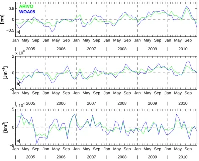
Fig. 2. Sensitivity test to estimate the climatology uncertainty for (a) GSSL, (b) GOHC and (c) GOFC during 2005–2010. To fill gaps at depth as well as to evaluate anomaly fields, two different climatologies are used, i.e. either ACLIM (green) or WOA05 (blue, see text for more details).

Jan Apr Jul Oct Jan Apr Jul Oct Jan Apr Jul Oct Jan Apr Jul Oct Jan Apr Jul Oct −0.5

0 0.5

[cm]

2004 2005 2006 2007 2008

| | | | | |

Fig. 3. GSSL anomaly (60◦S–60◦N, 10–1500 m) during 2004–2008 based on three different gridded fields, i.e. ARIVO (green, Argo plus other data, Ifremer), from Scripps Institution of Oceanograph (blue, Argo only) and MOAA (red, Argo plus other data, Japan Agency for Marine-Earth Science and Technology). The data have been downloaded from the Argo web page (www.argo.ucsd.edu).

3 Error estimation

A sound interpretation of GOIs requires a careful estima-tion of errors. Errors contain measurement noise, system-atic instrumental biases, sampling and data processing errors, including the effect of unresolved ocean variability scales

(5)

other hydrographic data (ARIVO delivered by Ifremer, and MOAA delivered by JAMSTEC), and one product including Argo-only measurements (delivered by Scripps Institution of Oceanography). Detailed information on the gridded fields can be found on the Argo webpage. We chose to evaluate the comparison during the time period 2004 to 2008 for con-sistency. Amplitudes of interannual fluctuations differ from one product to another (Fig. 3). Although the evaluation of GSSL in Fig. 3 is more or less based on the same data base, differences are clearly visible. These differences lead to a large spread of the estimation of global steric trends ranging from nearly 0 mm yr−1to about 1 mm yr−1. This simple ex-ercise already shows that a sensitivity study due to the data processing is vital.

3.1 Error bars estimated for global GOIs

The error_i,j2 on the averaged physical parameter8iin every 5◦×10◦×3 month box using the formulation of Breterthon et al. (1976) can be written as

_i,j2 =_X1

i,j

Ai,j−1

σ_i,j2 ,

whereσ_i,j2 is the variance of8iwithin each box, respectively. This takes into account the reduced number of degrees of freedom to estimate the error on the mean value for a given box (through the covariance matrix). Note that this effect is not negligible. Assuming independent observations would reduce the error variance by more than 10 %. To evaluate the error for the global estimation, we need to take into account errors for all boxes. Boxes that have less than 10 observations are associated with a variance error equal to the total variance of the physical parameter. The global mean errorsE(t )2can be then calculated as follows:

E(t )2=

X i,j

_i,j2 M2_i,j

X i,j

M2_i,j . (3)

An additional source of uncertainties arises from the choice of the climatology used to fill vertical gaps and to calculate the anomaly fields. As discussed in Sect. 2 and shown in Fig. 2, the climatological uncertaintyE_clim2 is small, but not negligible. This needs to be included in the error bar calcula-tion. To estimate the value forE_clim2 , the standard deviation of the difference between the two time series using either ACLIM or WOA05 (see Fig. 2) has been derived for each GOI. Thus, the total errorEtotal(t )2on GOIs can be defined as

Etotal(t )2=E(t )2+Eclim2 . (4) This total error includes the uncertainties due to the data processing and the choice of the reference climatology, but

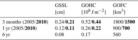
Table 1. Uncertainties of GOIs during 2005 and 2010 (bold) for different time averages, i.e. 3 month, 1 yr and 6 yr. See text for more details. These values do not take into account uncertainties induced by remaining systematic errors in the Argo observing system.

GSSL GOHC GOFC [cm] [108J m−2] [km3] 3 months (2005/2010) 0.24/0.21 0.52/0.44 1800/1500 1 yr (2005/2010) 0.12/0.11 0.26/0.22 900/700 6 yr 0.08 0.17 560

it does not take into account possible unknown systematic measurement errors not precisely corrected for in the de-layed mode Argo quality control (e.g. pressure errors, salin-ity sensor drift). Our method can be used, however, to discuss sampling issues for the estimation of GOIs and their errors. Table 1 shows the uncertainties due to data processing and the climatology of global mean GOIs during 2005 and 2010 for different time averages. Errors clearly decrease with the growing coverage of Argo. For example, uncertainties of 3-monthly GOHC are±0.52×108J m−2during the year 2005 and reduce to±0.44×108J m−2 during 2010. Estimating annual mean GOIs from the currently complete Argo observ-ing system can be performed with an accuracy of±0.11 cm for GSSL,±0.22×108_{J m}−2_{for GOHC, and}_±_{700 km}3_for GOFC.

3.2 Global trend error estimation

The method of weighted least square fit is used to retrieve 2005–2010 GOI trends. The trend of each GOI time series is evaluated using a weighted least square solution where the weights are the error bars of our GOIs given by Eq. (4) (see Appendix A). Note that error bars obtained from Eq. (4) only involve errors due to the sampling, data processing meth-ods and climatology uncertainties. Thus, the uncertainty of global trend estimations might increase in future studies as systematic errors due to unknown instrument biases have not been taken into account.

(6)

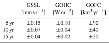
Table 2. A “forecast calculation” of the uncertainties of global trend estimations assuming GOI error bars during the year 2010 while applying Eq. (A1) (Appendix) for 10 and 15 yr, together with the trend uncertainties of the current GOI estimation during 2005– 2010. These values do not take into account uncertainties induced by remaining systematic errors in the Argo observing system.

GSSL GOHC GOFC [mm yr−1] [W m−2] [km3yr−1] 6 yr ±0.15 ±0.10 ±90 10 yr ±0.07 ±0.04 ±40 15 yr ±0.04 ±0.02 ±20

Note that our estimations provide an estimation of errors on the trend over a given time period. Such trends, even if they are statistically significant, cannot be interpreted as long-term climate trends as they also include the effect of interannual signals. This is clearly the case for the GOFC trend.

4 Testing the method

Altimeter sea level observations are a useful and nearly global observational record over the ice-free oceans that have been shown to be correlated well with in situ SSL and OHC (e.g. Willis et al., 2004; Guinehut et al., 2006). Maps of mean sea level anomalies (MSLA) are ideal to validate our simple box averaging method based on irregular sampling. Using the high-resolution altimeter measurements as a proxy for in situ GOI estimations (SSL and OHC) has already been performed in previous studies (Lyman and Johnson, 2008; Roemmich and Gilson, 2009). Although satellite MSLA fields are not truly global and have possibly undefined er-rors and also contain mass (bottom pressure) signals (Ponte, 1999; Wunsch et al., 2007), they are a very useful proxy to test our simple box averaging method. We used grid-ded fields downloagrid-ded from the AVISO webpage (merged gridded product, www.aviso.org). Weekly AVISO maps of MSLA on a 1/3◦Mercator grid are subsampled at the loca-tions and time of the year of in situ data collected for all years during 2005 to the end of 2010 and compared with actual global MSLA (derived from the MSLA maps). Then global mean sea level anomalies have been calculated as described in Sect. 2. The comparison between the two global averages shows reasonable agreement and their 6 yr trends are consis-tent (Fig. 4). However, there are differences in annual and lower period variability among the curves. This test shows that our simple box averaging method depicts global mean changes reasonably well and can be used to assess GOIs for monitoring needs of the climate system.

5 Estimation of GOIs

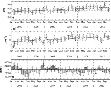
In this section, GSSL, GOHC and GOFC are derived from Argo data using the box averaging method discussed in Sect. 2 (Fig. 5). The 6-yr trend estimations are calculated as described in Sect. 3.2. Generally, the error decreases as the number of measurements increases and hence, the GOI errors decrease with time (Table 1).

A significant increase in GSSL can be observed from 2005 to 2010, with a trend of 0.75±0.15 mm yr−1(0.53 mm yr−1 for the Earth’s entire surface area, Fig. 5a). For this decade, values for in situ GSSL range from −0.5 to 0.8 mm yr−1 (e.g. Willis et al., 2008; Cazenave et al., 2009; Leuliette and Miller, 2009; von Schuckmann et al., 2009). The GOHC estimation shows a significant 6-yr increase, with a rate of 0.54±0.1 W m−2_{(0.38 W m}−2_{for the Earth’s entire surface} area, Fig. 5b). Our GOHC estimation is sligthly lower com-pared to the composite evaluated by Lyman et al. (2010) and to what was found in our earlier study (von Schuckmann et al., 2009). This can be due to the fact that the later period is confined to a period when the upper layers did not seem to be gaining much heat (e.g. Levitus et al., 2009; Cazenave and Llovel, 2010; Lyman et al., 2010). However, comparisons of GOHC and GSSL values from different studies are difficult to interpret as differences include the effect of interannual variability, instrumental biases or different data processing methods.

One important source of uncertainties in GOI estimations are due to the fact that patterns of interannual variability dif-fer among estimation methods (Domingues et al., 2008; Ly-man et al., 2010). Our results show that interannual fluctua-tions of GSSL and GOHC exist but are small (Fig. 5a and b). This is different for GOFC (Fig. 5c). Large interannual fluc-tuations dominate the time series, and the trend is very much dependent of these large interannual fluctuations. This im-plies that a longer time series is needed to extract a significant long-term trend for GOFC.

6 Conclusions

(7)

May Sep Jan May Sep Jan May Sep Jan May Sep Jan May Sep Jan May Sep −1

−0.5 0 0.5 1

AVISO MSLA [cm]

2005 | 2006 | 2007 | 2008 | 2009 | 2010

Fig. 4. Testing the method using gridded altimeter MSLA measurements (AVISO): gridded MSLA during 2005–2010 are subsampled to Argo profile positions and the simple box averaging method was applied. Global MSLA derived from the AVISO grid (bold line) is compared to its corresponding subsampled result (bold + dots). Dashed line marks November 2007, i.e. when initial Argo sampling was almost achieved.

Jan May Sep Jan May Sep Jan May Sep Jan May Sep Jan May Sep Jan May Sep −0.6

−0.2 0.2 0.6

[cm]

a)

2005 2006 2007 2008 2009 2010

| | | | | |

0 1

x 108

b)

[Jm

−

2 ]

2005 2006 2007 2008 2009 2010

| | | | | |

[km

3 ]

2005 2006 2007 2008 2009 2010

| | | | | |

c)

−20000 0 20000 40000

Fig. 5. Estimation of (a) GSSL, (b) GOHC and (c) GOFC. The calculation is based on the simple box averaging method applied to Argo measurements only. The 6-yr trends are of 0.75±0.15 mm yr−1, 0.54±0.10 W m−2and−80±90 km3yr−1, respectively. Error bars and trend uncertainties do not take into account remaining systematic errors in the Argo observing system.

We developed a method of evaluating GOIs that is easy to implement and can be used for a routine monitoring of the global ocean. With this method, a simple estimation of the errors on GOI estimations can be established and thus adequate interpretations and conclusions can be drawn. The estimation of GOIs based on our method are developed as part of the monitoring system in the frame of the

(8)

of±0.11 cm for GSSL,±0.22×108J m−2_{for GOHC, and} ±700 km3for GOFC. Assuming that the current Argo sam-pling is sustained for 15 yr, trends of GOIs could be per-formed with an accuracy of about±0.04 mm yr−1for GSSL, ±0.02 W m−2for GOHC and±20 km3yr−1for GOFC.

We have defined the error on GOIs based on sampling, data processing and climatology uncertainties only. Our er-ror estimations do not include remaining systematic biases in the Argo observing system (e.g. uncorrected drift of sen-sors, pressure errors). The sensitivity of GOIs to different proposed instrumental bias corrections (e.g. pressure offsets) needs to be tested now. Moreover, our trend estimations are estimated over a 6-yr time series only and are affected by interannual variability. Hence, an interpretation in terms of long-term climate signals remains questionable.

Appendix A

Weighted least square solution

The global trend estimation and its uncertainty are derived from a conventional weighted least square method:

The set of observationsyi=αiti+βcan be written as:

y=A0x, y=   

y1

.. .

yN

  , x=

_α

β

, A0=AW,

A=   

t1 1

..

. ...

tN 1

  , W=

   

1 E2 1

... 0

..

. . .. ...

0 ... 1

E_N2     .

The weighted least square solution where the weights are chosen to be the error bars of our GOIs (Eq. 4) can be written as:

X=(A0TA0)−1A0Ty.

Following Wunsch (1996), the variance of this estimation can be written as:

52=(A0W−1A)−1. (A1)

Acknowledgements. The research leading to these results has

received funding from the European Community’s Seventh Framework Programme FP7/2007-2013 under grant agreement no. 218812 (MyOcean). Comments from two anonymous review-ers greatly improved the manuscript. The authors would like to thank Fabienne Gaillard for providing us with the ISAS/ARIVO products and for various discussions improving the results as well as Mathieu Hamon and C´ecile Caban´es for useful discussions.

Edited by: T. Suga

The publication of this article is financed by CNRS-INSU.

References

Antonov, J., Levitus, S., and Boyer, T.: Steric sea level variations during 1957–1994: Importance of salinity, J. Geophys. Res., 107, C12, 8013, doi:10.1029/2001JC000964, 2002.

Antonov, J., Locarnini, R., Boyer, T., Mishonov, A., and Garcia, H.: World Ocean Atlas 2005, vol. 2, Salinity, NOAA Atlas NESDIS, vol. 62, edited by: Levitus, S., NOAA, Silver Spring, Md., 182 pp., 2006.

Boyer, T., Levitus, S., Antonov, J., Locarnini, R., and Garcia, H.: Linear trends in salinity for the world ocean, 1955–1998, Geo-phys. Res. Lett., 32, L01604, doi:10.1029/2004GL021791, 2005. Boyer, T., Levitus, S., Antonov, J., Locarnini, R., Mishonov, A., Garcia, H., and Josey, S. A.: Changes in freshwater content in the North Atlantic Ocean 1955–2006, Geophys. Res. Lett., 34, L16603, doi:10.1029/2007GL030126, 2007.

Bretherton, F., Davis, R., and Fandry, C.: A technique for objective analysis and design of oceanic experiments applied to mode-73, Deep-Sea Res., 23, 559–582, 1976.

Caban´es, C., de Boyer Mont´egut, C., Coatonoan, C., Ferry, N., Per-tuisot, C., von Schuckmann, K., Petit de la Villeon, L., Carval, T., Pouliquen, S., and Le Traon, P.-Y.: CORA (Coriolis Ocean Database for Re-analyses), a new comprehensive and qualified ocean in-situ dataset from 1990 to 2008 and its use in GLORYS, Joint Coriolis-Mercator Ocean Quarterly Newsletter, 37, 13–17, 2010.

Cazenave, A. and Llovel, W.: Contemporary sea level rise, Annual Review of Marine Science, 2, 145–173, 2010.

Cazenave, A., Dominh, K., Guinehut, S., Berthier, E., Llovel, W., Ramillien, G., Ablain, M., and Larnicol, G.: Sea level budget over 2003–2008: A reevaluation from GRACE space gravimetry, satellite altimetry and Argo, Global Planet. Change, 65, 83–88, 2009.

Church, J. A. and White, N. J.: Sea-level rise from the late 19th to the early 21st century, Surv. Geophys., 32, 585–602, doi:10.1007/s10712-011-9119-1, 2011.

Delcroix, T., Cravatte, S., and McPhaden, J.: Decadal variations and trends in tropical Pacific sea surface salinity since 1970, J. Geophys. Res., 112, C03012, doi:10.1029/2006JC003801, 2007. Durack, P. J. and Wijffels, S. E.: Fifty-year trends in global ocean salinities and their relationship to brad-scale warming, J. Cli-mate, 23, 4342–4362, doi:10.1175/2010JCLI3377.1, 2010. Domingues, C. M., Church, J. A., White, N. J., Gleckler, P. J.,

Wijf-fels, S. E., Barker, P. M., and Dunn, J. R.: Improved estimates of upper-ocean warming and multi-decadal sea-level rise, Nature, 453, 1090–1094, doi:10.1038/nature07080, 2008.

(9)

Gouretski, V. and Reseghetti, F.: On depth and temperature bi-ases in bathythermograph data: Development of a new correc-tion scheme based on analysis of a global database, Deep-Sea Res. Pt. I, 57, 812–833, 2010.

Guinehut, S., Le Traon, P.-Y., and Larnicol, G.: What can we learn from global altimetry/hydrography comparisons?, Geophys. Res. Lett., 33, L10604, doi:10.1029/2005GL025551, 2006.

Hansen, J., Nazarenko, L., Ruedy, R., Sato, M., Willis, J., Del Ge-nio, A., Koch, D., Lacis, A., Lo, K., Menon, S., Novakov, T., Perlwitz, J., Russell, G., Schmidt, G. A., and Tausnev, N.: Earth’s energy imbalance: Confirmation and implications, Science, 308, 1431–1435, doi:10.1126/science.1110252, 2005.

Le Traon, P.-Y. and Morrow, R.: Ocean currents and eddies, in: Satellite Altimetry and Earth Science, edited by: Fu, L.-L. and Cazenave, A., International Geophysics Series, 69, 171–215, 2001.

Leuliette, E. W. and Miller, L.: Closing the sea level rise bud-get with altimetry, Argo, and GRACE, Geophys. Res. Lett., 36, L04608, doi:10.1029/2008GL036010, 2009.

Levitus, S., Antonov, J., and Boyer, T.: Warming of the world ocean, 1955–2003, Geophys. Res. Lett., 32, L02604, doi:10.1029/2004GL021592, 2005.

Levitus, S., Antonov, J., Boyer, T., Locarnini, R., Garcia, H., and Mishonov, A.: Global ocean heat content 1955–2007 in light of recently revealed instrumentation problems, Geophys. Res. Lett., 36, L07608, doi:10.1029/2008GL037155, 2009.

Locarnini, R., Mishonov, A., Antonov, J., Boyer, T., and Garcia, H.: World Ocean Atlas 2005, vol. 1, Temperature, NOAA Atlas NESDIS, vol. 61, edited by: Levitus, S., NOAA, Silver Spring, Md, 182 pp., 2006.

Lyman, J. M. and Johnson, G. C.: Estimating Annual Global Upper-Ocean Heat Content Anomalies despite Irreg-ular In Situ Ocean Sampling, J. Climate, 21, 5629–5641, doi:10.1175/2008JCLI2259.1, 2008.

Lyman, J. M., Good, S. A., Gouretski, V. V., Ishii, M., John-son, G. C., Palmer, M. D., Smith, D. M., and Willis, J.: Ro-bust warming of the global upper ocean, Nature, 465, 334–337, doi:10.1038/nature09043, 2010.

Ponte, R. M.: A preliminary model study of the large-scale seasonal cycle in bottom pressure over the global ocean, J. Geophys. Res., 104, 1289–1300, 1999.

Roemmich, D. and Gilson, J.: The 2004–2008 mean and annual cycle of temperature, salinity, and steric height in the global ocean from the Argo Program, Prog. Oceanogr., 82, 81–100, doi:10.1016/j.pocean.2009.03.004, 2009.

Roemmich, D. and the A. S. Team: Argo: The Challenge of Con-tinuing 10 Years of Prog. Oceanogr., 20, 26–35, 2009.

Trenberth, K.: The ocean is warming, isn’t it?, Nature, 465, p. 304, 2010.

Trenberth, K. E. and Fasullo, J. T.: Tracking Earth’s energy, Sci-ence, 328, 316–317, 2010.

von Schuckmann, K., Gaillard, F., and Le Traon, P.-Y.: Global hy-drographic variability patterns during 2003–2008, J. Geophys. Res., 114, C09007, doi:10.1029/2008JC005237, 2009.

Willis, J., Roemmich, D., and Cornuelle, B.: Interannual variabil-ity in upper ocean heat content, temperature, and thermosteric expansion on global scales, J. Geophys. Res., 109, C12036, doi:10.1029/2003JC002260, 2004.

Willis, J., Chambers, D., and Nerem, R.: Assessing the globally av-eraged sea level budget on seasonal to interannual timescales, J. Geophys. Res., 113, C06015, doi:10.1029/2007JC004517, 2008. Willis, J. K., Lymann, J. M., Johnson, G. C., and Gilson, J.: In situ data biases and recent ocean heat content variability, J. Atmos. Ocean. Tech., 26, 846–852, 2009.

Wong, A., Keeley, R., Carval, T., and the Argo Data Management Team: Argo quality control manual version 2.6, Argo data man-agement, http://www.argodatamgt.org, 2010.

Wunsch, C.: The ocean circulation problem, Camebridge Univer-sity Press, New York, 114–118, 1996.