www.ocean-sci.net/7/1/2011/ doi:10.5194/os-7-1-2011
© Author(s) 2011. CC Attribution 3.0 License.
Ocean Science
Absolute Salinity, “Density Salinity” and the
Reference-Composition Salinity Scale: present and future use in the
seawater standard TEOS-10
D. G. Wright1,†, R. Pawlowicz2, T. J. McDougall3, R. Feistel4, and G. M. Marion5 1Bedford Institute of Oceanography, Dartmouth, NS, B2Y 4A2, Canada
2Department of Earth and Ocean Sciences, University of British Columbia, Vancouver, BC V6T 1Z4, Canada 3CSIRO Marine and Atmospheric Research, G.P.O. Box 1538, Hobart, TAS 7001, Australia
4Leibniz-Institut f¨ur Ostseeforschung, Seestraße 15, 18119 Warnem¨unde, Germany 5Desert Research Institute, Reno, NV, USA
†deceased
Received: 30 May 2010 – Published in Ocean Sci. Discuss.: 31 August 2010
Revised: 2 December 2010 – Accepted: 18 December 2010 – Published: 6 January 2011
Abstract. Salinity plays a key role in the determination of the thermodynamic properties of seawater and the new TEOS-101 standard provides a consistent and effective ap-proach to dealing with relationships between salinity and these thermodynamic properties. However, there are a num-ber of practical issues that arise in the application of TEOS-10, both in terms of accuracy and scope, including its use in the reduction of field data and in numerical models.
First, in the TEOS-10 formulation for IAPSO Standard Seawater, the Gibbs function takes the Reference Salinity as its salinity argument, denotedSR, which provides a mea-sure of the mass fraction of dissolved material in solution based on the Reference Composition approximation for Stan-dard Seawater. We discuss uncertainties in both the Refer-ence Composition and the ReferRefer-ence-Composition Salinity Scale on which Reference Salinity is reported. The Refer-ence Composition provides a much-needed fixed benchmark but modified reference states will inevitably be required to improve the representation of Standard Seawater for some studies. However, the Reference-Composition Salinity Scale should remain unaltered to provide a stable representation of salinity for use with the TEOS-10 Gibbs function and in cli-mate change detection studies.
Second, when composition anomalies are present in sea-water, no single salinity variable can fully represent the
in-Correspondence to: R. Pawlowicz ([email protected])
1TEOS-10: international Thermodynamic Equation of Seawater
2010, www.teos-10.org.
fluence of dissolved material on the thermodynamic proper-ties of seawater. We consider three distinct representations of salinity that have been used in previous studies and discuss the connections and distinctions between them. One of these variables provides the most accurate representation of den-sity possible as well as improvements over Reference Salin-ity for the determination of other thermodynamic properties. It is referred to as “Density Salinity” and is represented by the symbolSAdens; it stands out as the most appropriate repre-sentation of salinity for use in dynamical physical oceanogra-phy. The other two salinity variables provide alternative mea-sures of the mass fraction of dissolved material in seawater. “Solution Salinity”, denotedSAsoln, is the most obvious exten-sion of Reference Salinity to allow for composition anoma-lies; it provides a direct estimate of the mass fraction of dis-solved material in solution. “Added-Mass Salinity”, denoted SAadd, is motivated by a method used to report laboratory ex-periments; it represents the component of dissolved material added to Standard Seawater in terms of the mass of mate-rial before it enters solution. We also discuss a constructed conservative variable referred to as “Preformed Salinity”, de-notedS∗, which will be useful in process-oriented numerical
modelling studies.
1 Introduction
The relationships between the chemical composition, con-ductivity, salinity, and thermodynamic properties of IAPSO Standard Seawater, modified only by the addition and re-moval of pure water through dilution and evaporation (here-after denoted SSW), are now defined to the best available pre-cision by a linked series of standards. Millero et al. (2008a) (hereafter referred to as MFWM) define a fixed Reference Composition (RC) as an estimate of the relative mole frac-tions of the components of dissolved material in SSW, and link this to the conductivity/salinity relationship defined by the Practical Salinity Scale 1978 or PSS-78 (UNESCO, 1981). Among other benefits, salinities can now be ref-erenced on an absolute or mass fraction scale, directly re-lated to the dissolved material within seawater. Thermody-namic properties, including density, are consistently linked to salinity by a thermodynamic equation of state for seawater (TEOS-10) represented in terms of a Gibbs function formu-lation, which itself is based on a comprehensive evaluation of all relevant data (Feistel, 2008, 2010; Feistel et al., 2010a, b; IOC et al., 2010).
However, as discussed here, our direct knowledge of the true chemical composition of SSW has an uncertainty which is equivalent to a mass fraction salinity uncertainty of order 0.05 g kg−1, whereas modern conductivity-based measure-ment techniques can routinely resolve spatial variations of as little as 0.002 g kg−1in salinity. Work done subsequent to MFWM already suggests the presence of small system-atic deviations in the relative composition of SSW compared to the RC. Further, even leaving aside the issue of the ex-act composition of SSW, the composition of real seawater from different parts of the world oceans is known to differ slightly from the composition of SSW, which is derived from North Atlantic surface water. These composition anomalies are in fact the single largest source of errors in estimates of the thermodynamic properties of real seawater when TEOS-10 equations are used under the assumption that composi-tion anomalies are negligible. We are thus led to pose two questions: first, is the fixed composition model and the as-sociated absolute salinity scale an appropriate enduring ap-proach, and second, can we adapt the TEOS-10 formulation to incorporate additional information about these composi-tion variacomposi-tions.
Regarding the Reference Composition defined by MFWM, it is clear that this can serve as a useful benchmark even though the connection with SSW is limited by both data uncertainties and the variability in SSW itself. Further, it is obvious that changes in the definition of the RC would have the potential to cause confusion in the future. Thus, al-though refinements of the RC will inevitably be required for particular applications (e.g., Pawlowicz, 2010; Pawlowicz et al., 2010), we argue that the set of molar ratios defining the RC should be established as a fixed benchmark.
The use of a fixed absolute salinity scale and the SSW Gibbs function formulation to characterize arbitrary seawa-ters, affected by biogeochemical processes in the ocean, is less obvious. Although the full ramifications of this choice are not yet definitively known, recent investigations (Millero et al., 2008a, b, 2009; McDougall et al., 2009; Pawlowicz, 2010; Pawlowicz et al., 2010; Feistel et al., 2010a, b; Seitz et al., 2008, 2010a, b) have yielded estimates of the magni-tude of the resulting errors in different circumstances, as well as some details of the operational issues that arise. Here we discuss our present understanding of these issues.
These recent investigations have also highlighted some conceptual difficulties that are not present when discussion is limited to SSW. The term “Absolute Salinity” has been defined for Reference-Composition Seawater (RCSW) and SSW in MFWM and used as a measure of dissolved mate-rial in seawater in previous publications (McDougall et al., 2009; Feistel et al., 2010a). In this context, the term “abso-lute” is taken as implying a true mass fraction measure. This is in contrast to the traditional Practical Salinity, which is defined as a function of conductivity ratio at reference condi-tions with the function chosen to give a result proportional to Chlorinity, and with the proportionality constant chosen for consistency with past practice, rather than a best estimate of the mass fraction of dissolved material. However, the mean-ing of “Absolute Salinity” has not yet been precisely defined for seawaters with composition anomalies. Here we consider seawaters with composition anomalies and show that in this case the absolute salinity can be characterized in a number of different ways. A family of salinity variables is defined and a consistent notation introduced to facilitate the discussion of their features and interrelationships.
is determined as the sum of Preformed Salinity and an appro-priately defined anomaly.
In Sect. 2, we briefly review the set of salinity variables that have been used in recent studies and in Sect. 3 we con-sider issues associated with SSW in the absence of composi-tion anomalies. The accuracy of the Reference-Composicomposi-tion Salinity Scale is reviewed and an argument is presented that future updates of the Reference-Composition Salinity Scale should be avoided in order to provide the required stability of the measurement scale. In Sect. 4 we consider various repre-sentations of the dissolved material in seawater that includes composition anomalies. Several representations of the mass fraction of dissolved material in seawater, including the Den-sity Salinity, are defined and approximations used to estimate them are considered. Additional considerations regarding the validity of using Density Salinity as an argument of the Gibbs function are also discussed. A framework for the consider-ation of the effects of composition anomalies in numerical models is proposed in Sect. 5. Section 6 provides a summary and conclusions.
2 A family of salinity variables
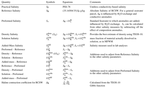
In this article, we refer to seven measures of salinity: Chlo-rinityCl, Practical SalinitySP, Reference SalinitySR, Den-sity Salinity SAdens, Solution Salinity SAsoln, Added-Mass Salinity SAadd, and Preformed Salinity S∗. Each of these
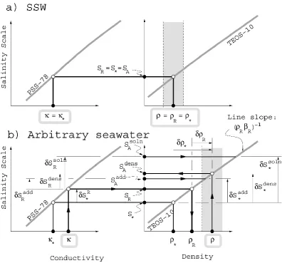
salinity variables have been discussed in previous publica-tions (Millero et al., 2008a, b, 2009; McDougall et al., 2009; IOC et al., 2010; Pawlowicz, 2010; Pawlowicz et al., 2010), although not necessarily in a consistent or explicit manner. Their definitions will be formalized here. An explanation of the notation used and a figure to illustrate the relations between the various measures of salinity and density is pro-vided in Appendix A.
Chlorinity is the oldest of the salinity measures considered and is still a corner-stone in the study of dissolved material in seawater. Based on the principle of constant relative propor-tions it provides a measure of the total amount of dissolved material in seawater in terms of the concentration of halides. Practical Salinity has been the internationally accepted stan-dard for the representation of ocean salinity for the past 3 decades; for SSW it is basically a scaled version of Chlo-rinity estimated via the measurement of conductivity. Ref-erence Salinity is defined by MFWM to provide a measure of the mass fraction of dissolved material in SSW, and incor-porates the result of a century of study into the true compo-sition of seawater. The most practical way to estimate Ref-erence Salinity over the Neptunian range of conditions is to determine Practical Salinity and multiply by the fixed scale factor (35.16504/35) g kg−1. We note however that Refer-ence Salinity provides the best estimate of the mass fraction of solute in a seawater sample only if it has the composition of SSW. The last 4 Salinity Variables have been introduced
to more accurately deal with seawater that includes compo-sition anomalies with respect to SSW and are discussed in Sect. 4. Preformed SalinityS∗is constructed to be as
conser-vative as possible; it is designed to be insensitive to biogeo-chemical processes that affect the other types of salinity to varying degrees. For SSW, five of the salinity variables are equal, the exceptions being Chlorinity and Practical Salinity. As discussed by MFWM and others before them, if the relative proportions of dissolved material in seawater can be assumed constant, then Chlorinity provides a suitable proxy measure of dissolved material in seawater. It is defined as 0.3285234 times the ratio of the mass of pure silver (g) re-quired to precipitate all dissolved halides (chloride, bromide and iodide) in seawater to the mass of seawater (kg). Prob-lems with this measure of salinity are that Chlorinity must be measured by a skilled technician using a precise silver standard, the process is time consuming, and Chlorinity can-not be measured in situ, but only on collected water sam-ples. Also, the approach assumes a fixed (or at least pre-cisely known) composition of dissolved material in order to convert from Chlorinity to a dissolved mass fraction. Finally, the reproducibility of the silver standard and its traceability to a reliable SI reference is unclear.
Practical SalinitySPwas introduced 30 years ago as a re-placement for Chlorinity that addresses the first set of issues, but does not properly account for composition anomalies or allow traceability to the SI (Lewis, 1981). Practical Salinity is relatively easy to measure using now standard equipment, measurements are more precise and less time consuming than measurements of Chlorinity and accurate measurements can even be made in situ. The success of the method relies on the fact that for a fixed composition at specified tempera-ture and pressure, the conductivity is related in a one-to-one manner to the mass ratio of dissolved material in seawater and the conductivity ratio relative to a standard can be pre-cisely measured using robust techniques. Further, reliable standards are routinely available in numbered batches from the Standard Seawater Service (Bacon et al., 2007). In prac-tice, a polynomial relation was empirically determined to cal-culate ChlorinityClfrom a measured conductivity ratio and the resulting estimate of Chlorinity was converted to Practi-cal Salinity usingSP=1.80655Cl/(g kg−1), a choice that was made to maintain numerical continuity with historical salin-ity estimates atCl=(35/1.80655) g kg−1. The strict defini-tion of Practical Salinity requires that measurements be made at a pressure ofP=101 325 Pa andt=15◦C on the IPTS-682 temperature scale (t=14.996◦C on the ITS-903scale), but al-gorithms are available to convert from conductivity measure-ments at other pressure and temperature values so this is not a serious restriction as long as any composition anomalies present do not corrupt these conversion relations (Feistel and Weinreben, 2008). This is unlikely to be a serious concern
in the open ocean given that Pawlowicz (2010) estimates the maximum error in the temperature correction to be of order 0.0004 g kg−1when converting from 1◦C to 25◦C for North
Pacific Intermediate Water where composition anomalies are near maximum.
MFWM list several reasons that a revised estimate of salinity is now desirable. Five of these are: (1) to introduce a chemical composition model for SSW which can be used in defining the Gibbs function for seawater at low salinities; (2) to adjust the numerical value of the standard measure of salinity to be as close as possible, given measurement un-certainties, to the true mass fraction of dissolved material in SSW (i.e., its absolute salinity); (3) to formally allow for ar-bitrarily large or small values of salinity, (4) to overcome theT−P limitations of PSS-78, and (5) to officially allow mass fraction units for salinity and make oceanographic pa-pers more readable for the wider scientific community. To achieve these goals, they define a stoichiometric composi-tion model for SSW (the Reference Composicomposi-tion or RC), de-termine a “best estimate” of the mass fraction of dissolved material corresponding to this model at a Practical Salin-ity of 35, and specify an algorithm to determine a consis-tent estimate of the mass fraction of dissolved material in a sample of arbitrary salinity with the RC. The resulting mea-sure of salinity is referred to as the Reference-Composition SalinitySR(or simply Reference Salinity) and the scale on which the Reference Salinity is measured is referred to as the Reference-Composition Salinity Scale (RCSS). By using this approach, the Reference Salinity provides an estimate of the mass fraction of dissolved material in any seawater sam-ple by approximating it with seawater that has the Reference Composition defined by MFWM.
The use of a single absolute salinity variable to represent the material dissolved in a seawater sample is most appro-priate for SSW because it has a nearly fixed relative com-position. In fact, IAPSO Standard Seawater can be consid-ered as a physical realization of the Reference-Composition Seawater construct. Nevertheless, it should be noted that the composition of SSW from different batch numbers must vary as a consequence of its natural origin, and the exact magni-tude of these changes is presently unknown. Even as a con-ductivity standard there are indications from the intercom-parison of field measurements that batch-specific offsets of up to about 0.003 in Practical Salinity occur (Kawano et al., 2006), although the reasons for this have been disputed (Ba-con et al., 2007). Seawaters of arbitrary origin may include much larger composition anomalies that will further distin-guish them from RCSW. Since these anomalies are of scien-tific interest it is appropriate to consider them separately.
For a seawater sample of arbitrary composition, a single measure of absolute salinity is too simple to fully describe its properties. This point is most obvious if one considers the dissolution in seawater of a substance that affects density and other properties but does not affect conductivity (silicic acid and sugar provide examples for which this is a
reason-able approximation). In such a case, the Practical SalinitySP and the Reference SalinitySR, both of which are functions of the conductivity of seawater, each remain almost unchanged even for significant changes to the mass fraction of solute present in the solution. Similarly, Chlorinity is almost unaf-fected by the addition of typical composition anomalies (real seawater anomalies do not normally include halides but they do slightly modify the mass of solution). Thus, none of these quantities provide a measure of the change in the mass frac-tion of dissolved material in seawater that allows for general composition anomalies.
In fact, there is still no practical means to actually deter-mine the mass fraction of dissolved material in water for the general case. Hence a precise and easily obtained measure of the amount of dissolved material in seawater is required as an extension of Reference Salinity to allow for compo-sition anomalies. Any extension must agree precisely with the Reference Salinity when the dissolved material has the composition assigned to Standard Seawater. In addition, it is desirable to introduce a measure of salinity that is trace-able to the SI (Seitz et al., 2008, 2010a, b; IOC et al., 2010) which is not achieved by the introduction of Reference Salin-ity (Seitz, 2010b). We shall argue that the introduction of “Density Salinity”SAdensaddresses both of these issues.
It should be noted that MFWM interchangeably used the words “Absolute Salinity” and the symbol SA for what we now recognize as two different absolute salinity measures, Solution Salinity and Density Salinity. For most of that paper MFWM discuss SSW for which these measures of salinity are equivalent to within measurement uncertainties, but with an implication of Solution Salinity. However, in Sect. 7 of MFWM they consider the influence of composition anoma-lies and they use the words Absolute Salinity and the symbol SA for what we now call Density Salinity with the symbol SAdens.
We now consider uncertainties associated with the defini-tion of the RCSS and the representadefini-tion of the salinity of SSW. We discuss the effects of composition anomalies in Sect. 4.
3 The Reference-Composition Salinity Scale and the salinity of SSW
of a water sample whose composition precisely matches the SSW that was analyzed in the 1970s, when most of the con-ductivity and density measurements underlying both EOS-804and TEOS-10 were made. Since the different measures of absolute salinity are defined to be equal for SSW it is ap-propriate to use the symbolSA without a superscript in this section.
3.1 Uncertainties in the Reference-Composition Salinity Scale
The Reference Composition includes all important compo-nents of seawater having mass fractions greater than about 1 mg kg−1in seawater with a Practical Salinity of 35 that can significantly affect either the conductivity or the density. All mass fractions were defined using the best available infor-mation for concentrations and molar masses in 2008, and the RC was carefully adjusted to be in charge balance. The un-certainty in the molar masses alone gives rise to a mass frac-tion salinity uncertainty of about 1 mg kg−1(Millero et al., 2008a), but there are larger sources of uncertainty.
The most significant ions present in seawater but not included in the RC are Li+ (∼0.18 mg kg−1) and Rb+ (∼0.12 mg kg−1). Dissolved gases N2 (∼16 mg kg−1) and O2(up to about 8 mg kg−1) are not included since they are highly variable and neither have a significant effect on den-sity or on conductivity. In addition, N2remains within a few percent of saturation for the measured temperature in almost all laboratory and in-situ conditions. However, the dissolved gas CO2(∼0.7 mg kg−1) and the ion OH−(∼0.08 mg kg−1) are included in the RC in spite of their small concentrations because of their important role in the equilibrium dynamics of the carbonate system. Changes in OH−concentration that
are commonly expressed in terms of pH involve conversion of CO2to and from other ionic forms and affect conductivity and density. The RC concentrations of the carbonate system components were determined by taking the known total alka-linity, assuming equilibrium with the levels of CO2gas in the atmosphere in 1976, and then using known mathematical re-lationships for the equilibrium chemistry. Concentrations of the major nutrients Si(OH)4, NO−3, and PO
3−
4 are assumed to be negligible in SSW. Dissolved Organic Matter (DOM) is typically present at concentrations of 0.5–2 mg kg−1in the ocean, but its composition in seawater is complex and poorly known. Although its concentration in SSW is unknown it is likely to be smaller because of the filtration used in the man-ufacturing procedure. It is not included in the RC.
The Reference-Composition Salinity Scale (RCSS) is de-fined implicitly in MFWM by an algorithm that is used to specify the Reference Salinity SR. The Reference Salin-ity is defined to provide an estimate of the (mass frac-tion) absolute salinity of seawater with the RC. It is given 4EOS-80: International equation of state of seawater 1980
(Fo-fonoff and Millard, 1983)
in terms of two end members, pure water defined as Vienna Standard Mean Ocean Water (VSMOW; IAPWS, 2001) and KCl-normalized Reference-Composition Seawa-ter (RCSW) which is seawaSeawa-ter with the Reference Com-position att=25◦C, P=101 325 Pa that has been adjusted to a Practical Salinity SP of 35 (exactly) through the ad-dition or removal of VSMOW. The Reference Salinities of VSMOW and KCl-normalized RCSW are defined to be ex-actly 0 g kg−1and 35.16504 g kg−1, respectively. The Refer-ence Salinity of an arbitrary sample of RCSW is then de-fined by assuming conservation of dissolved material dur-ing the addition or removal of pure water to the sample. If a sample with massm1requires the addition or removal of a mass m2 (>0 for addition and <0 for removal) to bring its Practical Salinity to SP=35, then its Reference Salinity is (1+m2/m1)×35.16504 g kg−1. Reference Salinity is not modified by changes in temperature or pressure that are made without mass exchange. Note that in reality, there are small changes in the relative composition of a seawater sample as-sociated with changes in temperature, pressure and concen-tration. This is because equilibrium chemistry relationships between some of the constituents depend on these factors. Consequently, Reference Salinity is perhaps best thought of as a potential mass fraction salinity that is obtained under the particular reference conditions discussed above.
As noted by MFWM, the value of the Absolute Salinity SAof RCSW can be related to the atomic weights of the con-stituents and the Chlorinity of the sample by:
SA= [0.3285234×(AAg/hAi)×(XCl+XBr)]−1Cl , (1) whereXCl andXBr are the mole fractions of chlorine and bromine in the sea salt,AAg is the atomic weight of silver, hAiis the mole-weighted mean atomic weight of solute with the Reference Composition and Cl is the Chlorinity of the sample of RCSW. The mole fractions of dissolved material in RCSW are precisely defined and Eq. (1) is exact for this composition. Thus, for specified Chlorinity the only source of uncertainty in the determination ofSAfrom Eq. (1) is the uncertainty associated with the atomic weights. For a typ-ical sample with Practtyp-ical Salinity near 35 (Chlorinity near 19.374 g kg−1) the resulting uncertainty inSAis only about 0.001 g kg−1(Millero et al., 2008a).
However, estimates of salinity rely on conductivity mea-sures, so MFWM rewrite Eq. (1) as
SA=uPSSP, (2)
where the RCSS scale factoruPSis defined by
uPS= [0.3285234×SonCl×(AAg/hAi)×(XCl+XBr)]−1,(3)
Millero, 2010), and approximate SonClby the value 1.80655 (g kg−1)−1, which is the value appropriate to SSW (Dauphi-nee, 1981; Culkin and Smith, 1981). This choice is supported by the fact that the RC was defined as a “best approximation” to the composition of SSW. However, there are uncertainties associated with this value. In particular, any modification of the estimated composition of SSW would imply a differ-ence between its composition and the fixed composition of RCSW, and this could imply a change in the best estimate of SonClthat should be used for the latter in Eq. (1), and thus a deviation of the ratioSA/SRfrom unity for RCSW. The un-certainty associated with SonCl is by far the largest source of uncertainty associated with the determination of the Ab-solute Salinity of RCSW using Eqs. (2) and (3).
We note however that our interest in Eqs. (1–3) is based on the fact that they provide a means to estimate the absolute salinity of SSW rather than a specific interest in the absolute salinity of the theoretical water type referred to as RCSW. Consequently, it is of interest to consider the true uncertain-ties associated with the use of these equations for this pur-pose. To investigate this issue, we take a slightly different approach to that presented by MFWM.
Consider a sample of SSW that was used in the deter-mination of PSS-78 and assume that its Practical Salin-ity has been precisely determined. Since the relation SP=1.80655Cl/(g kg−1) was used as a definition to convert between Chlorinity measurements and Practical Salinity for this particular vintage of SSW, we can use this relation as an identity here. Thus, given the Practical Salinity of our SSW sample, we know the value of its Chlorinity. Using Eq. (1), we now determine the Absolute Salinity of RCSW that has the same value of Chlorinity and we use this value as an es-timate of the absolute salinity of our SSW sample.
There are subtle but important points to note about the modified interpretation given in the previous paragraph. First, the resulting value of Absolute Salinity is recognized as an estimate of the absolute salinity of the SSW sample rather than that of the ideal RCSW sample used in the estimation procedure. Second, the estimate of the absolute salinity of the SSW sample with measured Practical Salinity is given by Eqs. (2) and (3) and is thus exactly the same as the esti-mate of the absolute salinity of the RCSW sample with the same Practical Salinity. Third, the use of SonCl=1.80655 (g kg−1)−1for RCSW has been completely eliminated. Con-sequently, neglecting the small uncertainties associated with the atomic weight estimates, determination of the uncertainty associated with the use ofSR as a measure of the absolute salinity of SSW is reduced to consideration of the accuracy of the RC as a representation of SSW.
We emphasize that use of Eqs. (2) and (3) to estimate the absolute salinity of a sample of RCSW involves uncertain-ties associated with the use of the value of SonCl for SSW but it does not involve any uncertainties associated with the mole fractions since these are precisely defined for RCSW. On the other hand, use of Eqs. (2) and (3) to directly estimate
the absolute salinity of a sample of SSW as described above involves uncertainties associated with the use of RCSW as a model for SSW, but it does not involve any uncertainties associated with the value of SonCl since this value is pre-cisely known for the SSW samples of interest. Since our true interest is in estimating the absolute salinity of SSW, the use of Eqs. (2) and (3) to directly estimate the absolute salin-ity of a sample of SSW is preferred here and we continue to consider the uncertainties associated with using RCSW as a model for SSW.
Even at the time that the RC was defined it was clear that uncertainty in the true composition of SSW was larger than the scientific requirements for precision in a salinity measure, which are about 0.002 g kg−1. Recently, Seitz (2010a and personal communication 2010) have estimated the sulfate (SO24−) mass fraction of a sample of KCl-normalized SSW to be 2.702±0.022 g kg−1. This range of values overlaps with the Reference Composition value of 2.71235 g kg−1 so it does not suggest any need to revise the RC at this time. How-ever, it also includes a lower bound of 2.68 g kg−1which can-not currently be ruled out as a representation of the properties of SSW. If the estimated sulfate mass fraction in SSW were reduced from 2.71235 g kg−1 to 2.68 g kg−1(a reduction of 337 µmol kg−1), then upon using the approach of MFWM in which the sodium (Na+) concentration is adjusted to achieve charge balance, the estimated absolute salinity of the result-ing modified RCSW would be reduced from 35.16504 g kg−1 to 35.11114 g kg−1. This suggests the possibility that a future change in the estimated absolute salinity of SSW withSP=35 could be as large as 0.054 g kg−1, more than an order of mag-nitude larger than the precision of Practical Salinity measure-ments and one third of the difference between 35.16504 and 35, i.e., the difference betweenSR/(g kg−1) andSPfor KCl-normalized RCSW.
The above discussion deals with the accuracy of the RCSS for the determination of the absolute salinity of SSW. That is, it deals with the issue of how accurately the Reference Salinity, determined from conductivity, represents the mass fraction of dissolved material in solution for the ideal case of a sample of 1970s SSW. We have seen that the inaccuracies may be as large as 0.05 g kg−1which is substantially larger than the contributions to the mass fraction of dissolved ma-terial from composition anomalies that we consider in some detail in Sect. 4. However, these offsets will affect all salin-ity values proportionately and are accounted for in the defini-tion of the Gibbs funcdefini-tion for SSW, whereas the composidefini-tion anomalies discussed in Sect. 4 vary spatially and directly in-fluence horizontal pressure gradients. In the next section, we consider whether the uncertainties in the absolute salinities of SSW and RCSW might result in a need to update the RCSS in the future.
3.2 Will the RCSS need to be updated in the future?
The above discussion emphasizes the uncertainty in the use of the Reference Salinity to estimate the mass fraction of dis-solved material in 1970s SSW. It motivates us to ask what should happen if an improved estimate of the composition of this vintage of SSW is determined in the future. At first, it would seem natural to update the Reference Composition and hence the estimate of the mass fraction of dissolved material in SSW. This would in turn change both the RCSS and the uncertainty associated with it. This approach would be nec-essary if we required the RCSS to always provide the best possible estimate of the mass fraction of the salts dissolved in standard seawater without additional adjustments. Below, we argue that even if at some time in the future an improved estimate for the composition of SSW is definitively deter-mined, it would still be highly undesirable to modify the RC and along with it the RCSS.
There are two primary reasons that updating the RCSS should be avoided. First, we note that changes in Refer-ence Salinity of order 0.002 g kg−1(i.e., changes in Practical Salinity of order 0.002) are detectable in the ocean and salin-ity changes have been interpreted as indications of climate change (Levitus, 1989; Joyce et al., 1999; Wong et al., 1999; Dickson et al., 2002, 2003; Curry et al., 2003). Thus it is highly desirable for climate change studies to use a measure of salinity that will not change by this amount unless there is a true change in the salinity of seawater. Since the precision of Reference Salinity estimates is of this order, it provides a suitable measure if the definition of the RCSS remains un-changed. However, the uncertainty of order 0.05 g kg−1 as a measure of the mass fraction of dissolved material in sea-water introduces the possibility that the RCSS could be re-vised several times by amounts considerably in excess of 0.002 g kg−1 as estimates of the mass fractions in RCSW are improved. Such changes recorded in data bases and in publications could be misinterpreted as signatures of climate
change by investigators who are unaware of changes in the measurement scale. The potential for confusion is substan-tial and obviously undesirable. It should be avoided.
The second primary reason to avoid changes in the RCSS relates to the methods used to estimate the parameters in the TEOS-10 Gibbs potential function for seawater. The param-eters in this function have been determined to provide cor-rect results for SSW for specified values of Absolute Salin-ity, temperature and pressure, with the Absolute Salinity ex-pressed on the current RCSS (recall that Reference Salin-ity is our best estimate of the Absolute SalinSalin-ity of SSW). If this scale were to be changed, then the input salinity argu-ment for the Gibbs function would be changed without any real change in the properties of a sample. Consequently, the Gibbs function would have to be modified to obtain the same thermodynamic properties with a modified salinity input. Al-though the required change is simple (it can be implemented by changing a single parameter) the possibility that some ver-sions of computer code used to evaluate the Gibbs function would not be correctly updated is rather large. Even if the updates were somehow made in every existing version of the code, changes in the RCSS over time would require that dif-ferent parameters be used in the Gibbs function for difdif-ferent time periods. Clearly the chance of introducing confusion through such changes is large.
Based on the above discussion, we conclude that it is desir-able to avoid any changes in the definition of the RCSS. For-tunately, such changes should not be necessary. This is be-cause the Reference Salinity is needed first to determine the salinity input to the Gibbs function and second as a measure of the mass fraction of dissolved material in seawater. Mea-surements on the current scale can serve both purposes very well. As already noted, maintenance of a fixed RCSS is de-sirable for applications of the Gibbs function to estimate the density and other thermodynamic properties of SSW since the Gibbs function has been constructed to provide correct results with the salinity specified on the RCSS. So the only concerns are related to use of the RCSS to provide a measure of the true mass fraction of dissolved material in seawater.
should continue to be archived in national data bases (see IOC et al., 2010). This practice of storing results for a mea-sured quantity but publishing results based on another related quantity is analogous to the present practice of archiving in situ temperature even though potential temperature is used for most analyses. This recommendation of IOC et al. (2010) is primarily intended to avoid confusion in data bases but it also means that the influence of any modifications of our best mass fraction estimates will be easily and consistently ap-plied to both future data and past data that has been archived since Practical Salinity was defined 3 decades ago. In fact, since Practical Salinity is related to Chlorinity by the simple relationSP=1.80655Cl, any improvement in mass fraction estimates will also be easily applied to all of the Chlorinity data collected during the century before the introduction of Practical Salinity.
4 The characterization of seawaters of arbitrary composition
4.1 Salinity variables for the representation of arbitrary seawater
The differences between the compositions of SSW and RCSW are important in accurately determining the true ab-solute salinity of SSW, and would therefore be important in (e.g.) determining the best possible estimate of the total salt content of the oceans. On the other hand, the Gibbs func-tion has been defined based on salinity measurements rep-resented on the RCSS so the thermodynamic properties of SSW determined from the Gibbs function will be accurate even if the RCSS provides a slightly incorrect estimate of the mass fraction of dissolved material in SSW. However, as sea-water circulates within the world oceans, its composition un-dergoes additional changes due to biogeochemical processes. The magnitudes of these changes are generally smaller than our uncertainty in the absolute salinity of SSW, but these anomalies are systematic and measurable, and their neglect results in errors in the representation of geographic changes in the thermodynamic properties of seawater. In contrast to any inaccuracies associated with the RCSS, these anomalies cannot be accounted for in the determination of the Gibbs function for SSW and they cannot be corrected for through a uniform scale factor applied to salinity estimates. In partic-ular, their neglect results in systematic errors in basin-scale density gradients, and thus in inferred basin-scale transports. Consequently, it is important to consider how these anoma-lies can be characterized. In this section, we discuss how the composition of seawater changes, and different methods of incorporating these changes in measures of salinity that can be used to describe arbitrary seawaters.
We limit consideration to changes that will affect salin-ities at amounts larger than about 0.001 g kg−1. Anoma-lies associated with the carbonate system (positive and neg-ative) tend to be largest due to the influences of air–sea ex-change and biological cycling (Brewer and Bradshaw, 1975;
Pawlowicz, 2010). Their effects on the components of the RC can be adequately parameterized using just the total al-kalinity (TA) and dissolved inorganic carbon (DIC) contri-butions, although they typically result in changes to the rel-ative concentrations of all components of the carbonate sys-tem. In addition, there may be anomalies for species that are not present in the RC. These include nutrients, of which the most significant are silicic acid and nitrate. Fortunately, TA, DIC, Si(OH)4and NO−3 are all routinely measured in hydro-graphic programs. Finally, the actual composition anomaly must involve parameters that are not routinely measured, since arbitrary changes in TA and NO−3 must be compen-sated in some way to preserve charge balance. The most im-portant process contributing to changes in TA in the deep ocean is likely the dissolution of CaCO3 (Sarmiento and Gruber, 2006), although other processes (e.g., sulfate reduc-tion; Chen, 2002) may be at work, particularly in coastal and marginal seas. Pawlowicz (2010) chooses to balance charge in his model through the addition or removal of Ca2+with the caveat that other processes are recognized to be important at least under some conditions. Comparison with observations reveals that the resulting estimates of Ca2+ are accurate to within about 0.8 mg kg−1.
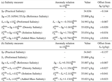
Pawlowicz et al. (2010) use the above approach in a model study; they represent the major contributions to composition anomalies relative to SSW by specifying the anomalies in four components: TA, DIC, NO−3 and Si(OH)4, with anoma-lies in Ca2+estimated from the requirements of charge bal-ance. The largest anomalies occur in the North Pacific. To motivate the following discussion we refer to Table 1a and b where numerical values for the different salinity variables that we are about to discuss are provided for a North Pacific scenario. A full description of this table will be provided be-low, but it is useful to note at this stage that the numerical differences between the different salinity variables are of or-der 0.01 g kg−1, significantly larger than the precision with which Practical Salinity is measured (0.002 g kg−1).
Table 1. Salinity corrections for water from the deep North Pacific, withδρR=0.015kg m−3, normalized to (a) SR=35g kg−1, and
(b)S∗=35 g kg−1.δρR=ρ−ρRis the estimated difference between the true density and the density evaluated from the Reference Salinity
using the TEOS-10 Gibbs function. The corresponding Density Salinity anomalyδSRdens(often denotedδSAin other papers) is given by
δSRdens=δρR/(ρRβR). The relations given in the second column are derived from formulae given in Pawlowicz et al. (2010) (see also IOC
et al., 2010).
(a) Salinity measure Anomaly relation Value Offset from toδSRdens SR/(g/kg)
SP(Practical Salinity) – 34.836 −0.164
SR=(35.16504/35)SP(Reference Salinity) – 35.000 g/kg –
S∗=SR+δSR∗(Preformed Salinity) S∗−SR≈−0.35δSRdens 34.993 g/kg −0.007
SAdens=SR+δSdensR (Density Salinity) SdensA −SR≈1.0δSRdens 35.020 g/kg +0.020
SAsoln=SR+δSRsoln(Solution Salinity) SAsoln−SR≈1.75δSdensR 35.034 g/kg +0.034
SAadd=SR+δSRadd(Added-Mass Salinity) SAadd−SR≈0.78δSRdens 35.016 g/kg +0.016
(b) Salinity measure Anomaly relation Value Offset from toδSRdens S∗/(g/kg)
SP(Practical Salinity) – 34.843 −0.157
S∗(Preformed Salinity) – 35.000 g/kg –
SR=S∗+δS∗R(Reference Salinity) SR−S∗≈0.35δSRdens 35.007 g/kg +0.007
SAdens=S∗+δS∗dens(Density Salinity) SAdens−S∗≈1.35δSRdens 35.027 g/kg +0.027
SAsoln=S∗+δS∗soln(Solution Salinity) SAsoln−S∗≈2.1δSRdens 35.041 g/kg +0.041
SAadd=S∗+δSadd∗ (Added-Mass Salinity) SAadd−S∗≈1.13δSdensR 35.023 g/kg +0.023
The considerations leading to the definition of SSW76 are discussed in detail by Pawlowicz (2010) and Pawlowicz et al. (2010). Briefly, both the RC and SSW76 are based pri-marily on analyses of SSW done in the 1970s. However, the borate and carbonate components represent significant contributions to the composition of SSW that were not sys-tematically investigated and MFWM and Pawlowicz (2010) adopt different choices for these components. MFWM es-timate these components under the assumption of equilib-rium with atmospheric conditions at 25◦C whereas Pawlow-icz (2010) sets the DIC content of SSW76 to force the den-sity to match that of in situ North Atlantic surface water, and (scanty) information about the true DIC content of SSW. The result is that the DIC specified by Pawlowicz (2010) is 2080 µmol kg−1, significantly higher than the RC value of 1963 µmol kg−1. Correspondingly, the estimated mass fraction of dissolved material in KCl-normalized seawater is increased from 35.16504 g kg−1 to 35.17124 g kg−1. In this context, it is noteworthy that Brewer and Bradshaw (1975) determined the DIC content of SSW batch P61 to be 2238 µmol kg−1and Millero et al. (1976b, 1978) report a value of 2226 µmol kg−1 in SSW used to determine the equation of state. Although there is significant uncertainty associated with the carbonate components of SSW, it is very
likely that the value of DIC corresponding to SSW76 is more representative of the analysed batches of SSW than the value corresponding to the RC; this choice also simplifies the equa-tions used to model interrelaequa-tionships between the different salinity variables by avoiding the need to introduce offsets in the relations presented in Table 1a and b.
argument of the Gibbs function must be expressed on the RCSS which was determined using the RC. In practice, salin-ity will be determined from Reference Salinsalin-ity plus anoma-lies in observational studies. Reference Salinity is defined using Eq. (8) so it is automatically expressed on the RCSS. Strictly speaking, the salinity anomalies determined by the formulae of Pawlowicz et al. (2010) should be multiplied by the factor 35.16504/35.17124 to express them on the RCSS, but this adjustment is entirely negligible for the small anoma-lies that occur in the open ocean.
To proceed further, we must carefully define what is meant by terms like “Absolute Salinity” when composition anoma-lies are present. This has not been done rigorously in previ-ous publications.
The approach of Millero and co-workers has been to ar-gue that changes in the mass fraction of dissolved material in seawater relative to SR are adequately approximated by δSA=(ρ–ρR)/(βRρR) whereβRandρRare the haline con-traction coefficient and density atS=SRdetermined from EOS-80 or TEOS-10 (the differences are negligible in this context). This approximation for the mass fraction of dis-solved material is now referred to as Density Salinity and denoted bySAdenswith the incrementδSAdenoted byδSRdens. The approach is supported by previous work (Millero, 1975; Chen and Millero, 1986) indicating that density changes of natural waters are affected primarily by the mass of added material, with the relative composition providing only a sec-ondary effect. This definition naturally reverts to the exist-ing definition of Reference Salinity as anomalies from SSW tend to zero since the density varies smoothly as composition anomalies tend to zero.
However, the limitations and biases of this approach are not well understood for seawater that includes anomalies from SSW. Previous verification has not systematically con-sidered the range of composition variations that occur in the ocean and since the physical/chemical characteristics of different solutes can vary greatly, it is not really clear how Density Salinity is related to the mass fraction of dis-solved material in seawater with arbitrary composition. Nor were changes in conductivity considered, which would affect Practical and Reference Salinity. In fact, we will see below that the difference between Density Salinity and Reference Salinity does not necessarily provide a good approximation for the anomalies in the mass fraction of dissolved material in seawater. Thus, although it will be argued that Density Salinity is well-suited to most physical oceanographic ap-plications, an alternative measure of salinity is required to provide a precise measure of the mass fraction of material dissolved in seawater.
To develop a more rigorous definition of mass frac-tion salinity that will apply in the presence of composi-tion anomalies and agree with the definicomposi-tion established in MFWM when no anomalies are present, we first re-examine the procedure followed by MFWM for SSW. The basic prin-ciples used to determine the Absolute Salinity of SSW are:
1. Addition or removal of pure water (i.e. dilution or evaporation) until SP=35.000 (or equivalently Cl=19.374 g kg−1),
2. Adjustment of the sample to chemical equilibrium at the reference conditions,t=25◦C and P=101 325 Pa, without exchange of mass, under which conditions the Absolute Salinity of the sample can be determined from Eqs. (2) and (3), and
3. Determination of the Absolute Salinity of the original sample as the mass of dissolved material in the adjusted sample divided by the total mass of the original sample. The obvious first steps in any definition of Absolute Salinity for anomalous compositions are then to standard-ize the concentration and adjust to equilibrium conditions att=25◦C andP=101 325 Pa. Unfortunately a precise
ad-justment to the conditions used for SSW is not possible be-cause the chemical equilibria in the solution will inevitably be affected to some degree by the anomalous solute. How-ever, operationally effective definitions are possible. Below, we discuss a conceptual approach followed by operationally practical approaches.
A crude standardization could be achieved simply by ad-justing the Chlorinity of the solution to 19.374 g kg−1. In this caseSPwould not in general be equal to 35.000 as it would for SSW because of the influence of composition anomalies on conductivity. Also, the total mass of solution, and hence the Chlorinity, is influenced by the presence of anomalous material so this approach to standardization is imprecise and will be inaccurate for large anomalies. A normalization ap-proach that is less affected by composition anomalies can be achieved (at least conceptually or in numerical calculations) by adjusting the chloride molality, the total number of moles of chloride per kg of solvent, instead of Chlorinity. Unlike Chlorinity, the chloride molality is not influenced by the ad-dition of anomalous solute that does not react with water; there is a weak influence if the added solutes react with wa-ter since they reduce the amount of wawa-ter by a small amount. It should be noted here that the separation between what is pure water and what is dissolved material is not totally clear, but this is not a serious issue at the level of accu-racy that we currently require (∼1 ppm in density and salin-ity). In particular, one might question whether H3O+ (the form that H+ actually takes in water) and OH− are solute or solvent but it makes little difference at this level of accu-racy. We have already noted that OH− is included as
that pOH (=14−pH) is near 6. Thus, the concentration of H3O+is roughly two orders of magnitude less than that of OH−. Hence although H
3O+ is considered as solute, it is not explicitly included in the RC because its contributions to density and salinity are far below the level of current concern. For consistency with the normalization used in the def-inition of Reference Salinity, we normalize to the chlo-ride molality of SSW76 that has a Chlorinity of 19.374. This choice gives a chloride molality of 0.556642 mol kg−1 (=19.734631 g chloride per kg H2O). Thus for consistency with the definition of Absolute Salinity in the absence of composition anomalies, we add or subtract massm2of pure water to adjust the original seawater sample of massm1 to a chloride molality of 0.556642 mol kg−1. We refer to this adjustment as chloride-normalization. We now divide the dissolved material (all material not in the pure water nent of the solution) into two components. The first compo-nent includes the chloride compocompo-nent plus each of the other components of SSW76 in the same mole ratios as defined for SSW76. The mass of solute in a chloride-normalized solution of SSW76 is 36.45335 g/(kg H2O) ((35.17124 g so-lute)/(1000 g solution−35.17124 g solute)). The second component includes all remaining dissolved material. Note that negative contributions from the chemical species in SSW are permitted in this second part although the total concentra-tion of any species is non-negative. We now assume that the total mass of solute in this normalized solution can be deter-mined and ismsolute. The mass of solvent in the normalized solution is thenmsolvent=m1+ m2–msolute. The total mass of the first component of solute ism3= 0.03645335×msolvent= 0.03645335×(m1+m2–msolute) and that of the second com-ponent ism4 = msolute–0.03645335 msolvent = 1.03645335 msolute–0.03645335 (m1+m2). In principlem4may be neg-ative (e.g., when some of a species in SSW is removed from solution).
Given the above information, the mass fraction definition of Absolute Salinity used by Millero et al. (2008a) can be extended to include composition anomalies in a (concep-tually) very straightforward manner. The absolute salinity of the chlorinormalized solution can then be simply de-fined as the mass of material dissolved in the solution di-vided by the total mass of the solutionmsolute/(m1+m2). The mass fraction of dissolved material in the original solution is then determined as before under the assumption of salt conservation during the addition or removal of pure water and is given by (1+m2/m1)×msolute/(m1+m2)=msolute/m1 or (m3+m4)/m1. We refer to this as the Solution Salinity, and denote it as SAsoln, where “soln” refers to the fact that the mass of dissolved material is determined after it reaches equilibrium in solution. This definition is consistent with the definition of Absolute Salinity given by MFWM (see Sect. 3 above) for SSW and uses the same basic approach to extend the definition to allow for composition anomalies.
The separation of solute into the two components intro-duced above is of interest in its own right. Since chloride
does not take part in biogeochemical cycling and so is es-sentially a conservative variable, the component associated with the Reference Composition will be quasi-conservative following the ocean general circulation, analogous to other similarly constructed quasi-conservative tracers like N∗and NO∗(Sarmiento and Gruber, 2006). It has mass fraction ab-solute salinityS∗=m3/m1and will be referred to as the Pre-formed Salinity.S∗is modified by exchanges of water at the
ocean surface and by mixing in the ocean interior, but the effects of biogeochemical processes on it are deliberately ex-cluded. It is thus an ideal baseline to which material is added by biogeochemical processes. The remainder of the solute is referred to as the anomalous part. Again, we note that it is possible for the “remainder” to be negative as in the case when some of a SSW species is removed from solution.
We emphasize thatSAsolndeals with a solution in equilib-rium and treats all non-water components of seawater as dis-solved material. Consequently, when new material is added to solution, the change in mass of the dissolved material may deviate from the added mass. Perhaps the most obvious ex-ample occurs when CO2 is dissolved in water to produce a mixture of CO2, H2CO3, HCO−3, CO23−, H+, OH− and H2O, with the relative proportions depending on dissociation constants that depend on temperature, pressure and pH. Thus, the dissolution of a given mass of CO2in pure water essen-tially transforms some of the water into dissolved material. Similar situations occur for other dissolved materials; some may also release water upon dissolution, such as certain cal-cium minerals.
In contrast to the case for Solution Salinity, it is some-times useful to deal with the anomalous mass added to SSW directly. This is particularly true in laboratory experiments. If a mass madd of anomalous solute is added to a sam-ple of KCl-normalized (or equivalently chloride-normalized) SSW of mass mssw then a mass fraction absolute salinity may be defined as (0.03517124mssw+madd)/(mssw+madd), where 0.03517124mssw is the mass of dissolved material in the original sample of SSW, madd is the added mass of anomalous material andmssw+maddis the total mass of the final solution. We refer to this as Added-Mass Salinity, and denote it asSAadd. For Standard SeawaterSAaddis also consis-tent with the definition of Absolute Salinity for SSW given by MFWM since no mass is added in that case, but for seawa-ter of anomalous composition the mass of anomalous solute is determined before it is added to the solution rather than af-ter equilibrium conditions have been established for the new solution, as would be required for the Solution Salinity. Any chemical reactions of the added solute with the SSW solu-tion are therefore not considered for Added-Mass Salinity. That is, neither precipitation of species nor redistributions between solvent and solute have any effect on Added-Mass Salinity. It is therefore conceptually very different from So-lution Salinity and we will see below that it is also substan-tially different in practice.
laboratory, it is not straightforward to estimate for seawater with anomalous composition that is sampled from the ocean. Even if we assume that the composition of the final equi-librium state is known, one must still estimate the mass of anomalous solute prior to any chemical reactions with SSW. Since equilibrium states are independent of their history, any combination of chemical species that irreversibly evolve to the given sample composition is a potential candidate for the computation of Added-Mass Salinity, which therefore is highly ambiguous for a given final solution. Additional infor-mation must therefore be provided to resolve this ambiguity if Added-Mass Salinity is to be determined for ocean seawa-ter. Pawlowicz et al. (2010) provide an algorithm to achieve this estimate, at least approximately, once some assumptions about ocean biogeochemical processes are made. The de-tails are substantially more complicated than those required for Solution Salinity and will not be reproduced here. The main point that we wish to emphasize is that the difference between Solution Salinity and Added-Mass Salinity lies in the treatment of the anomalous contributions and that (as il-lustrated in Table 1a and b) these differences are important at the level of precision being considered here. In either case, the Preformed SalinityS∗can be uniquely determined from
the chloride molality. However, the numerical values of the salinity anomaliesδS∗solnandδS∗add which are added to Pre-formed Salinity S∗ to determine SAsoln andSAadd may differ
significantly.
To illustrate the magnitude and range of the numerical variations between different measures of salinity, we con-sider an extreme example. Deepwater composition anoma-lies from SSW in the open ocean are largest at depth in the North Pacific. For KCl-normalized seawater, TA is in-creased relative to SSW values by about 150 µmol kg−1, and DIC by 300 µmol kg−1. NO−
3 concentrations are as high as 40 µmol kg−1, and Si(OH)4 concentrations are as large as 170 µmol kg−1. The corresponding increase in Ca2+ is in-ferred to be 95 µmol kg−1to balance charge. Maximum den-sity anomalies relative to densities calculated usingSR and the TEOS-10 equation of state in this region are estimated to be about 0.015 kg m−3, both from direct measurements and using the model calculations of Pawlowicz et al. (2010). The approximate magnitude of the corrections to determine salin-ities of the different types defined above can be derived from this density anomaly using equations proposed by Pawlow-icz et al. (2010). The corrections and the numerical values of the different salinities are shown in Table 1a and b. Ta-ble 1a shows the changes to the various salinity variaTa-bles with respect to a Reference Salinity, while Table 1b shows the same salinity perturbations with respect to a Preformed Salinity. The salinity perturbations in Table 1a are appropri-ate for the estimation of various measures of absolute salin-ity when the Practical Salinsalin-ity (and hence Reference Salin-ity) is available as a measured quantity (using, for example the lookup table of McDougall et al. (2009) to determine the
corrections) while Table 1b is relevant to the consideration of biogeochemical effects.
Importantly, the model study of Pawlowicz et al. (2010) shows that, for the anomalies arising from ocean biogeo-chemical processes, correlations between the anomalies of different constituents are strong enough in all ocean basins that the linear relations given in column 2 of Table 1 ap-ply for all deep-ocean sites within an uncertainty of about 0.003 g kg−1, even though the exact nature of the composi-tion anomalies that produce the density anomalies can vary with geographic location. If the details of the composi-tion anomalies in TA, DIC, NO−3 and Si(OH)4 are known, then more accurate interrelationships can be derived using relatively simple formulas (Pawlowicz et al., 2010; IOC et al., 2010), two of which are reproduced below as Eqs. (9) and (10). In practice, measurements of conductivity and density, or of conductivity and concentrations of major non-conservative parameters (carbonate system and nutrients), along with a few assumptions about the nature of ocean bio-geochemical processes, are enough to specify the full seawa-ter system to a useful accuracy, including Density Salinity, Solution Salinity, Added-Mass Salinity and Preformed Salin-ity.
The largest deviations from Reference Salinity in Table 1a are for Practical Salinity, and it is largely this discrepancy that justifies the introduction of the Reference Salinity as a more accurate measure of absolute salinity. The next largest numerical offset from the Reference Salinity appears in So-lution Salinity which is roughly one quarter as large as the offset for Practical Salinity. The final salinity increase for Solution Salinity is significantly larger than for Added-Mass Salinity due to the incorporation of H+ and OH− into the
anomalous non-conservative contributions to the dissolved material. The values for the Density Salinity SAdens and Added-Mass SalinitySAadd are closest, and would generally lie (just) within typical measurement error of each other, a determination that is shown to also hold for a variety of lab-oratory results in Pawlowicz et al. (2010). The smallest de-viation from Reference Salinity occurs for Preformed Salin-ity. However, even this change is about double the precision to which Reference Salinity can be determined through con-ductivity measurements. Tables 1a and b emphasize the fact that the single largest factor limiting our knowledge of the spatial variations of thermodynamic properties (like density) is a correct estimation of the effects of compositional varia-tions.
4.2 The “Density Salinity” of seawater
In Sect. 2 we noted that the Density Salinity equals the Ref-erence Salinity by construction for the special case of SSW and therefore reproduces the MFWM estimate of the mass fraction of dissolved material in seawater in this case. It is also intended to be a useful measure of salinity effects in the general case when composition anomalies are present but this depends on whether its use with the Gibbs function for SSW returns sufficiently accurate results for density and other ther-modynamic quantities over the range of oceanographic con-ditions. Here we more rigorously define the Density Salin-ity as a numerical measure that returns the correct value of density when used as an argument of the Gibbs function at a selectedT−P reference point, and show that the density values returned at other temperatures and pressures are suffi-ciently accurate for practical usage. We then discuss alterna-tive methods by which it can be estimated that will be useful in practice.
First, note that for SSW, the TEOS-10 density is given by ρ=1
ν= 1 gP(SR,T ,P )
, (4)
wherev is the specific volume, gis the Gibbs function for SSW (Feistel, 2008; IAPWS, 2008) and the subscriptP in-dicates partial differentiation with respect to pressure at con-stant salinity and temperature. For SSW, evaluating Eq. (4) at fixedSRfor different values ofT andP will determine the correct values ofρ for a fixed seawater sample. Thus, mea-surement ofρat any specified values ofT,P and subsequent inversion of Eq. (4) to determineSRwill return the unique value ofSRappropriate to the sample. This unique value of SRis referred to as the Density Salinity of the SSW sample and is represented by the symbolSAdens. We wish to extend this definition to apply to seawater samples of arbitrary com-position, but in this case the values ofSRdetermined by mea-surements of the same sample at different values ofT and P are not guaranteed to be the same since thermal expan-sion and compressibility may be influenced by the presence of composition anomalies in ways that are not accounted for by Eq. (4). Consequently, to use this procedure to define a unique representation of salinity for a seawater sample of arbitrary composition, we must specify reference conditions at whichSdensA is to be determined. For reference conditions, we chooset=25◦C and P=101 325 Pa. Thus, for a sam-ple of general composition, with densityρ att=25◦C and P=101 325 Pa, the Density SalinitySAdens is defined by the implicit equation
ρ= 1
gP SAdens,298.15K,101325Pa
. (5)
In general, Eq. (5) must be solved numerically, as discussed in Feistel et al. (2010a). This is straightforward because it in-volves the zero of a monotonic function; a routine to perform the inversion is provided in the Sea-Ice-Air library (Wright
et al., 2010). SAdensis thus guaranteed to provide the correct value of density when used as an input to the Gibbs function representation, for any seawater composition at the reference values of temperature and pressure. Below, we show that if Density Salinity is defined by Eq. (5), then it can also be used as the salinity argument in Eq. (4) to determine reliable estimates of the density at other values of temperature and pressure. The demonstration of this point also shows that the value determined for Density Salinity is not sensitive to the choice of reference conditions so although a choice must be specified for strict consistency, this choice is not important in practice.
To be more specific regarding the need to specify refer-ence conditions for a seawater sample of arbitrary composi-tion, we note that if the density is correctly determined at any reference pointTR,PR, then we can determine the density at any other temperature and pressure from the equation
ρtrue SAdens,T ,P=ρ SdensA ,TR,PR
+
T Z
TR ∂ρ ∂T S
dens A ,t,PR
dt (6)
+ P Z
PR
∂ρ ∂P S
dens A ,T ,p
dp,
where the partial derivatives with respect to temperature and pressure are the true values for the water sample. When the Gibbs function is used to evaluate the density, away from the reference conditions, these derivatives are effectively re-placed by the corresponding derivatives for Standard Seawa-ter. The error associated with using the Gibbs function to determine density for an arbitrary seawater sample can there-fore be expressed as
1ρ SAdens,T ,P= T Z
TR
∂(ρ−ρSSW)
∂T S
dens
A ,t,PRdt (7)
+ P Z
PR
∂(ρ−ρSSW)
∂P S
dens A ,T ,p
dp
whereρSSWis the density determined by the Gibbs function formulation for SSW.
However, the basic results discussed below have also been confirmed using the LIMBETA model (Pawlowicz et al., 2010) with different parameterizations of compressibility ef-fects. Thus, although details are uncertain, the model cal-culations provide a useful indication of the magnitude of the effects of composition anomalies on the evaluation of density using the Gibbs function for SSW.
To provide a relevant example, we consider the effect of anomalies similar to those observed at depth in the North Pacific where the largest known deep ocean anomalies are found. Two (numerical) samples of seawater are created, the first representing Standard Seawater as discussed by Feis-tel and Marion (2007) and the second including composition anomalies corresponding to North Pacific Intermediate Water (Sect. 4.1 and Pawlowicz et al., 2010). The concentration of solute in the SSW sample is specified to giveSR=35 g kg−1. NPIW anomalies are then added to a duplicate sample to give a density anomaly of approximately 0.015 g m−3, similar to the maximum anomalies observed in the open ocean. Pure water is then added to this NPIW sample to adjust its den-sity to match that of the original SSW sample att=25◦C, P=101 325 Pa, so that the samples of SSW and slightly di-luted NPIW have identical Density Salinities.
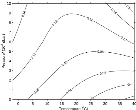
Using the algorithms included in the FREZCHEM model, modified to represent a closed system with respect to CO2 exchange, the density changes predicted for both the SSW sample and the diluted NPIW sample are now determined fort between−2◦C and 40◦C andP between 105Pa and 108Pa (roughly between the surface and 10 000 m below the ocean’s surface), and the density differences between the two samples are determined. If the temperature is below the freezing point of one or both samples then results are de-termined for metastable liquid states. The results are shown in Fig. 1 and indicate that the density difference between the two samples varies smoothly and is less than 0.2 g m−3over the full range of temperature and pressure conditions consid-ered. This difference is at least a factor of ten smaller than the smallest density differences that can be routinely detected using a densimeter and is certainly negligible for the present purpose. Uncertainties associated with the formulation of FREZCHEM (see, e.g., Marion et al., 2005) may signifi-cantly alter the details of Fig. 1, but they would not alter the main result that the errors associated with using the TEOS-10 Gibbs function, withSAdensas the salinity argument, to esti-mate density changes over the Neptunian range of temper-ature and pressure changes are negligible. Experimentation with the LIMBETA model (Pawlowicz et al., 2010) confirms that even with different choices for uncertain parameteriza-tions, the errors always remain less than 1 g m−3, which is still negligible for the present purpose.
FREZCHEM has also been used to estimate the corre-sponding anomalies in the specific heat capacity at atmo-spheric pressure and in the activity potential for the full Nep-tunian ranges of temperature and pressure. The differences between the specific heat capacity results for NPIW and
0
0
0.04
0.04
0.08
0.08
0.08 0.12
0.12
0.12
0.12 0.16
0.16 0.2
Temperature (oC)
Pressure/ (10
3 dbar)
0 5 10 15 20 25 30 35 40
0 1 2 3 4 5 6 7 8 9 10
Fig. 1. The estimated density difference (g m−3, ppm) between two water samples used to represent NPIW and SSW that have been adjusted to give identical densities att=25◦C andP=101 325 Pa. These estimates are obtained using the FREZCHEM model and should be treated as rough estimates. However, even given the asso-ciated uncertainties, the differences are negligible compared to the total density changes associated with composition anomalies in the open ocean.
SSW with the same Density Salinity are between 0.023 and 0.029 J kg−1K−1and are entirely negligible compared to the experimental uncertainty of 0.5 J kg−1K−1 for the specific heat capacity of pure water. In fact, even the total changes in heat capacity for an Absolute Salinity change of 0.025 g kg−1 is only about 0.12 J kg−1K−1, which is itself negligible com-pared to the measurement uncertainty, so we conclude that the influence of composition anomalies on specific heat ca-pacity is safely neglected. For the activity potential, total dif-ferences are between 3.5×10⁻⁵and 6×10⁻⁵with the largest values occurring at the highest temperatures and only a rela-tively weak dependence on pressure. These values are again negligible compared to the variations for each water sam-ple that are of order 3×10⁻²(values are in the range−0.40 to−0.43 for the range of oceanographic conditions consid-ered).