www.ocean-sci.net/6/431/2010/
© Author(s) 2010. This work is distributed under the Creative Commons Attribution 3.0 License.
Ocean Science
First images and orientation of fine structure from a 3-D seismic
oceanography data set
T. M. Blacic and W. S. Holbrook
University of Wyoming, Geology and Geophysics Department, 1000 E. University Ave., Laramie, WY 82071, USA Received: 11 September 2009 – Published in Ocean Sci. Discuss.: 20 October 2009
Revised: 11 February 2010 – Accepted: 29 March 2010 – Published: 20 April 2010
Abstract. We present 3-D images of ocean fine structure from a unique industry-collected 3-D multichannel seismic dataset from the Gulf of Mexico that includes expendable bathythermograph casts for both swaths. 2-D processing re-veals strong laterally continuous reflections throughout the upper∼800 m as well as a few weaker but still distinct re-flections as deep as∼1100 m. We interpret the reflections to be caused by reversible fine structure from internal wave strains. Two bright reflections are traced across the 225-m-wide swath to produce reflection surface images that illus-trate the 3-D nature of ocean fine structure. We show that the orientation of linear features in a reflection can be ob-tained by calculating the orientations of contours of reflec-tion relief, or more robustly, by fitting a sinusoidal surface to the reflection. Preliminary 3-D processing further illustrates the potential of 3-D seismic data in interpreting images of oceanic features such as internal wave strains. This work demonstrates the viability of imaging oceanic fine structure in 3-D and shows that, beyond simply providing a way vi-sualize oceanic fine structure, quantitative information such as the spatial orientation of features like fronts and solitons can be obtained from 3-D seismic images. We expect com-plete, optimized 3-D processing to improve both the signal to noise ratio and spatial resolution of our images resulting in increased options for analysis and interpretation.
Correspondence to: T. M. Blacic
1 Introduction
Ocean mixing processes are fundamentally 3-D in nature and vary in time on a wide range of scales. Features that af-fect thermohaline fine structure, such as internal waves, tidal beams, solitons, eddies, fronts, warm core rings, and turbu-lent patches, are expected to vary in both space and time. To study these kinds of features, oceanographers typically use a combination of surface measurements (e.g., satellite sea sur-face elevation and sursur-face temperature; Egbert et al., 1994; Ikeda and Emery, 1984), vertical profiles (by expendable in-struments, non-expendable lowered inin-struments, or moored instrument arrays; e.g., Cooper et al., 1990; Rudnick et al., 2003), and towed instruments that can take measurements either along one horizontal line or in a “tow-yo” sawtooth pattern (e.g., Rudnick and Ferrari, 1999; Klymak and Moum, 2007). These methods can capture large-scale patterns over a wide area or fine-scale patterns at a discrete location or depth. High frequency (100 kHz to 1 MHz) sonar methods can pro-vide 2-D images of backscattering in the upper ocean, which are interpreted to result from zooplankton, suspended sed-iment or sound-speed microstructure, and are used to map internal waves at shallow depths (e.g., Wiebe et al., 1997; Farmer and Armi, 1999). This array of measurement tech-niques leaves a large portion of the ocean (i.e., depths below a few hundred meters) under-sampled both laterally and ver-tically and opens the door to new ways of mapping oceanic fine structure.
(Holbrook et al., 2003). The reflections in the water column have been shown by Nandi et al. (2004) to primarily arise from water temperature fluctuations as small as 0.03◦C.
Al-though the images obtained can be intrinsically revealing of ocean structure, concurrent hydrographic measures (temper-ature/salinity profiles) are needed to ground truth the tem-perature variations highlighted by the reflections. Thus far, only 2-D seismic profiles have been processed for seismic oceanography (e.g., Holbrook et al., 2003; Tsuji et al., 2005; Nakamura et al., 2006; Biescas et al., 2008), although it is now standard in the oil industry to collect 3-D seismic data using ships that tow up to seventeen parallel hydrophone streamers. Here we present the first 3-D images of ocean fine structure obtained from a data set collected by a large oil company that includes concurrent expendable bathyther-mograph (XBT) profiles. This industry data set may be the first of its kind with coincident seismic and water tempera-ture measurements and represents an important step towards increasing cooperation and data sharing with the oil industry.
2 Methods
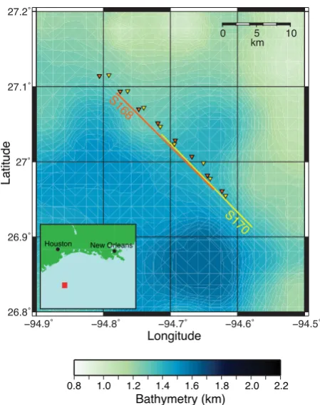
The data set consists of two 8-cable, 2-source 3-D swaths in the Gulf of Mexico off the coast of Texas that overlap in space and are separated in time by approximately two days. Swath S168, 20.3 km in length, was collected on 2 Febru-ary 2006, and swath S170, 19.0 km in length, was collected on 4 February 2006. Both were collected from NW to SE (Fig. 1). The seismic ship towed an array of 8 streamers spaced 60 m apart, each 4.65 km in length. Channel spacing along the streamers was 12.5 m; source spacing was 25 m for both sources with a flip-flop pattern (50 m when a sin-gle source is considered). This geometry results in common midpoint traces (CMPs) spaced every 6.25 m, representing the horizontal sample spacing of the resulting image in the along-swath direction. Across-swath sample spacing is de-termined by the source and receiver configuration. When each source is considered separately the sampled swath is 225 m wide, with an across-swath sample spacing of 15 m.
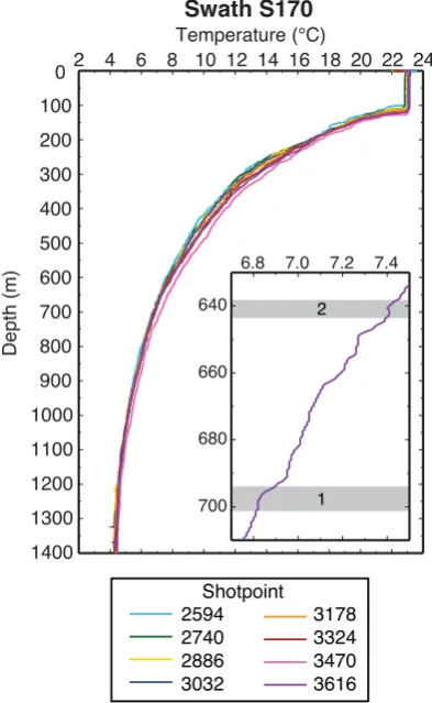
Eight expendable bathythermographs (XBTs) were de-ployed for each swath (Fig. 1). Casts were made from a second ship following the tail buoys at the end of the hy-drophone streamers towed by the seismic vessel. The XBTs were launched to coincide with certain shot points in the seis-mic data in order to achieve a uniform spacing. Temperature profiles for the XBTs coinciding with swath S170 are shown in Fig. 2.
For a first look at our 3-D data set we focus on swath S170, processing each of the eight cables as individual 2-D lines for each of the two sources, thus yielding 16 par-allel seismic sections (images). To mitigate the effect of streamer feathering we only used the near 32 traces for each shot-cable pair. This results in a stacking fold of 4 and im-ages that are noisier compared to full-fold imim-ages. However,
−94.9˚ −94.8˚ −94.7˚ −94.6˚ −94.5˚
26.8˚ 26.9˚ 27˚ 27.1˚ 27.2˚
0 5 10
km
Longitude
Latitude
Bathymetry (km)
0.8 1.0 1.2 1.4 1.6 1.8 2.0 2.2 S168
S170
New Orleans Houston
Fig. 1. Location map. Bathymetry has been interpolated from a
10grid (Smith and Sandwell, 1997) to 0.50grid spacing. Orange and yellow lines show locations of the CMP swaths; triangles show locations of the XBT casts.
0
100
200
300
400
500
600
700
800
900
1000
1100
1200
1300
1400
Depth (m)
2 4 6 8 10 12 14 16 18 20 22 24 Temperature (°C)
Swath S170
3178 3324 3470 3616
640
660
680
700
6.8 7.0 7.2 7.4
Shotpoint 1 2
2594 2740 2886 3032
Fig. 2. Temperature profiles from XBT casts for swath S170. Inset
shows blow-up of a portion of the profile for the XBT deployed nearest to the features shown in Fig. 6 (shotpoint 3616,∼0.7 km from features in Fig. 6). Grey bars highlight a temperature stair step (feature 1) and a small inversion (feature 2) which correspond with the reflection surfaces shown in Fig. 6.
sound speed of 1500 m/s corresponding to the average sound speed in the upper half of the water column.
We can estimate the resolution of our 2-D migrated im-ages in the along-swath direction by considering the horizon-tal sample spacing. Sampling theory states that the smallest wavelength we can expect to distinguish, λn, (without
tak-ing noise into account) is two times the trace spactak-ing (Sher-iff and Geldart, 1995), which for our survey geometry re-sults in λn=12.5 m. In the across-swath direction we must
consider the Fresnel zone to limit our resolution since mi-gration was only carried out in the along-swath direction. For water depths between 200 and 1200 m, airgun sources with a dominant frequency of 50 Hz, and assuming a sound speed of 1500 m/s in the water, the first Fresnel zone, R1, ranges from 55 to 134 m. However, because the outer por-tion of the Fresnel zone contributes relatively little energy to the reflection signal at a detector, we can consider the effective Fresnel zone,R1/
√
2 (Sheriff and Geldart, 1995), to limit the horizontal resolution in the across-swath
direc-tion to 39–95 m over the same depth range. Thus, we can discern features with wavelengths less than half the swath width, depending on the depth of the reflector. 3-D process-ing can improve the signal to noise ratio of the entire im-age volume, and with trace interpolation in the cross-swath direction and trace padding to reduce edge effects, 3-D mi-gration can improve the resolution limit in both along-swath and cross-swath directions to be on the order of twice the receiver spacing. Vertical resolution can be estimated as a quarter of the wavelength of the dominant frequency of the data (Widess, 1973). For our data, reflections have a fre-quency range of 30–100 Hz with the dominant frefre-quency at approximately 50 Hz. Assuming a sound speed of 1500 m/s results in a vertical resolution of∼8 m.
Using XBT temperature profiles and the robust parabola model of Thacker (2007) for estimating salinity at depth in the Gulf of Mexico, we can produce density profiles at each XBT cast location. We assumed hydrostatic conditions for converting depth to pressure, accounting for the change in density at each depth increment, and, as the temperature pro-files are relatively simple, we used a linear equation of state (Knauss, 1997) to calculate the density at depth. Isopyc-nals are plotted on top of that portion of the seismic image that overlaps with the XBT coverage in Fig. 3. The isopy-cnals are nearly horizontal across most of the image with a small downward dip beneath the XBT at shotpoint 3470. The density was also used, along with sound speed, to calcu-late impedance and reflection coefficient (e.g., Ruddick et al., 2009), which was then convolved with an estimated source wavelet to produce a synthetic section (Fig. 4).
We have also performed a rudimentary stack of the en-tire 3-D data volume for swath S170. This initial processing consisted only of 3-D grid application, reduction of coher-ent and random noise, flex binning, normal moveout (using the same sound speed profile as in our 2-D processing), band pass frequency filtering and median stacking. Because 3-D migration has not yet been performed, the Fresnel zone lim-its the horizontal resolution of the resulting image volume to∼55–135 m in all directions (for depths in the range of ∼200–1200 m); however, we can still gain some insight into the potential of 3-D seismic data sets for interpretation of oceanic processes from this first pass through a basic 3-D data processing flow.
3 Results and discussion
200
300
400
500
600
700
800
900
Depth (m)
0 1 2 3 4 5 6 7 8 9 10 11
Distance (km)
S170 Cable 4 - Density Contours (kg/m3)
1027.2
1027.4
1027.6
1027.8
3178 3324 3470 3616
Fig. 3. The portion of the migrated image of swath S170, cable 4, source 1, that overlaps with XBT coverage is shown with isopycnals
(kg/m3)plotted on top of the image. Yellow diamonds at the top indicate locations of XBT casts; numbers correspond to nearest shot point.
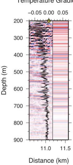
at depths of∼600–650 m, between∼3–4.5 km along swath at depths of∼500–550 m, and between∼9.2–10 km along the swath at a depth of∼550 m. A comparison between the temperature gradient (∇T) and the migrated image (Fig. 4) shows that the brighter reflections in the seismic image can be associated with peaks in∇T, although the alignment of reflections with peaks in∇T is not always perfect. The mi-grated image can also be compared to a synthetic section de-rived from the XBT data, shown on the right side of Fig. 4. The synthetic section shows the same first order trend of de-creasing reflection amplitudes with inde-creasing depth as seen in the data. In addition, many of the bright reflections in the synthetic section are aligned with bright reflections in the seismic data, although this is not always the case. This could be due to the fact that the boat from which the XBTs were cast was following the tail of the seismic streamer and so there was a time gap on the order of five minutes between when the shot was fired and when the XBT was cast at the approximate location of the shot. In that space of time the water continued to move, likely resulting in shifts in the lo-cation of reflectors. As can be seen in Fig. 1 there is also a spatial separation between the XBT casts and the seismic swath.
To investigate the source of the reflections we observe in our data, we must rely only on the XBT temperature pro-files and the slope of the reflections relative to our estimated isopycnals as we lack coincident salinity profiles. Although the reflections generally appear to follow isopycnals (Fig. 3), the temperature profiles (Fig. 2) show only a few small in-versions; they mostly consist of small stair steps with steep temperature gradients between thin layers of near-uniform
200
300
400
500
600
700
800
900
Depth (m)
11.0 11.5
Distance (km)
−0.05 0.00 0.05
Temperature Gradient
Fig. 4. Temperature gradient plotted on top of a portion of the
300
400
500
600
700
800
900
1000
1100
1200
Depth (m)
0 1 2 3 4 5 6 7 8 9 10 11 12 13 14 15 16 17
Distance along swath (km)
(a)
3616 3470
3324 3178
9 10 11 12 13
615
635
655
675
695
715
735
Distance along swath (km)
Depth (m)
(b)
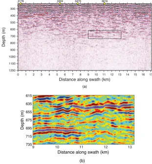
Fig. 5. (a) Migrated image of swath S170, cable 4, source 1. The images have been strongly smoothed but no relative gain control has been
applied. Black box outlines region shown in (b). Yellow diamonds at top indicate locations of XBT casts; numbers correspond to nearest shot point. (b) Selected portion of the migrated image shown in (a). Two strong continuous reflections (highlighted by pink lines) were tracked across the swath to make the reflection surfaces shown in Fig. 6.
temperature. We therefore suggest that the reflections are not caused by fine structure from thermohaline intrusions but instead result from reversible fine structure caused by inter-nal wave strain. Note that here we define “strain” follow-ing Thorpe (2005) as the vertical distance between two given isopycnal surfaces divided by their mean separation, and not in the formal sense of the strain tensor in an incompressible fluid. In this sense, a propagating internal wave causes zones of intensified or weakened “strain” (Thorpe, 2005, p. 60). The fine structure causing reflections in our data could also be a result of previous mixing with the boundaries between layers of well-mixed water perturbed by small-scale internal waves to produce the undulations we see in the reflections. This is not to say that any given reflection or reflection seg-ment in our images could or should be associated with a sin-gle internal wave with a specific source. The wavefield at any one time is a superposition of many waves with peaks and troughs corresponding to locations of constructive interfer-ence of those waves. Therefore, some additional information on currents or other sources of internal waves is needed when
interpreting the source of any particular reflection. For our data set, there is no additional oceanographic data available that could help us interpret a source for a reflection. How-ever, for illustrative purposes, we examined and calculated the orientation of one wave peak in order to demonstrate the feasibility of obtaining such information from 3-D seismic reflection data.
9.5 10.0
10.5 11.0
11.5 12.0
12.5 13.0
640
650
670 660
680
690
700
0 0.2 Across-swath distance (km)
Along-swath distance (km)
Depth (m)
−6 −4 −2 0 2 4 6
Depth variation (m)
0 0.2
9.5 10.0 10.5 11.0 11.5 12.0 12.5 13.0
0 0.2
Across-swath distance (km)
Along-swath distance (km)
1 2
1 2
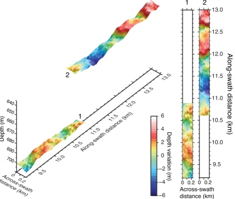
Fig. 6. Reflections 1 and 2, tracked in Fig. 5, are shown in 3-D
perspective view (left) and 2-D map view (right).
Reflection 1 was tracked across the swath from along-swath distanceX=9.2 to 10.9 km; reflection 2 was tracked from
X=10.6 to 13.0 km. The “flying carpet” surface images that result from combining the 16 2-D reflection tracks are shown in Fig. 6. Reflection 2 shows a greater degree of depth vari-ability compared to reflection 1, but the 3-D nature of both reflections can be easily discerned. In general, the reflec-tions display an egg carton-like surface of peaks and troughs, though some features have a more linear appearance.
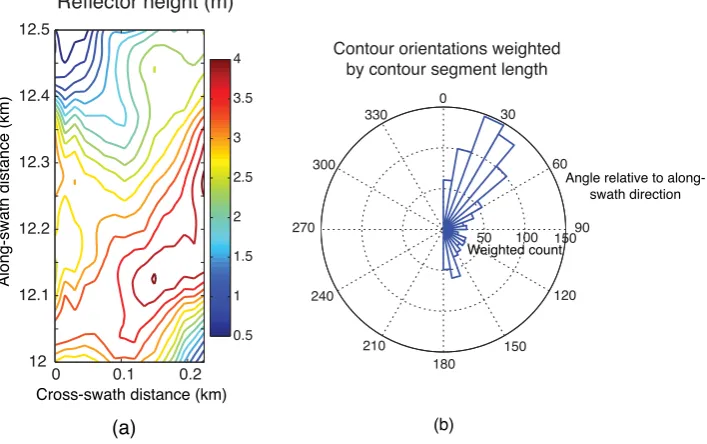
Orientation of fine structure that is more linear in appear-ance can be determined by several means. As an example, we can fit a line by eye to the single wave crest in reflection 2 between 12 and 12.5 km in the along-swath direction. It should be noted that in this example we are not attempting to say anything about wave properties in the region but are investigating how we might fit a local feature. Knowing that the azimuth of the seismic swath is∼134◦ gives us an az-imuth of∼169±5◦for this wave crest. More rigorously, we can draw contours of wave relief and determine the orienta-tion of each contour line segment, as shown in Fig. 7. Here we again focus on the portion of reflection 2 between 12 and 12.5 km along the swath. Before contouring, the data is first smoothed in the across-swath direction by applying a three point moving average filter. Orientations for the contour line segments are then weighted by line segment length and plot-ted in a rose diagram in Fig. 7b, which shows that the dom-inant direction of the feature is∼30◦from the along-swath direction, or∼164◦azimuth.
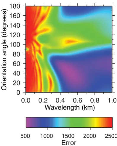
Another method for estimating reflection peak/trough ori-entation that does not depend on the chosen contouring algo-rithm is to fit a sinusoidal surface of the form
G=Asin(Kx+Ly+φ) (1)
to the reflection of interest, where A is the amplitude,φis the phase shift required to align the peaks (expressed as a frac-tion of the phase length),K= |1/λ|cosθ,L= |1/λ|sinθ,λ
is the wavelength, andθis the orientation angle of the peaks. We began by fitting a surface by eye to the same portion of re-flection 2 from 12 to 12.5 km along the swath, then adjusted
A,φ,λandθuntil a reasonably good fit was obtained (Fig. 8, center). We then setAto 1.55 km, corresponding to the best-fitting value chosen by eye, and calculated model surfaces for a range ofλandθ, allowing the best-fitting phase shiftφ
to be chosen for each (λ,θ )pair. The model with the mini-mum error, calculated as the sum of the squared differences between the model surface and the reflection surface, is then our “best” model (Fig. 8, right). The error surface, plotted in Fig. 9 as a function ofλandθ, is relatively simple with a clear global minimum, indicating that this is a robust way to estimate the orientation of linear peaks or troughs in a reflec-tion. Reflection peak/trough orientations for both the by eye fit and our best fit (azimuths of 171◦and 181◦, respectively) compare reasonably well to the values obtained by adding up contour segment orientations or simply fitting a line by hand. We note that lack of migration in the across-swath direc-tion does not affect the determinadirec-tion of wave orientadirec-tion by contour segments or sinusoidal surface fitting. Although the across-swath resolution of the image would be improved to ∼60 m with migration, this would have only a small effect on the location of the peaks and troughs and thus only a small effect on the orientation of the contour lines drawn or the rel-ative error of different surface models. Therefore, measuring wave orientations is an important application of 3-D seismic oceanography images even when migration of the data is not performed. However, due to the increase in noise in the rose diagram and in the error surface for surface fitting when mul-tiple features are included in the contouring, this method of determining wave orientation is best suited to easily discern-able targets such as solitary waves and fronts.
Reflector height (m)
0 0.1 0.2
12 12.1 12.2 12.3 12.4 12.5
Cross-swath distance (km)
Along-swath distance (km)
0.5 1 1.5 2 2.5 3 3.5 4
(a)
50 100 150
30
210
60
240
90 270
120 300
150 330
180 0
Contour orientations weighted by contour segment length
Angle relative to along-swath direction
Weighted count
(b)
Fig. 7. Reflection peak/trough orientation relative to the swath can be obtained from a topographic contour plot of tracked reflections such
as those shown in Fig. 6. (a) Contour plot of reflection relief for a portion of reflection 2 (see Fig. 6). (b) Rose diagram showing orientations of contour line segments relative to the along-swath direction. Histogram count has been weighted by contour line segment length.
Future work will include full 3-D processing of the data from both swaths including migration. This will place all CMP traces into grid boxes based on location, which will mitigate the streamer feathering problem and allow for greater and more uniform stacking fold. In general, once the stacking procedure has been optimized and 3-D migration has been performed, we expect to see an increase in the sig-nal to noise ratio as well as an increase in our options for imaging and interpreting the structure of internal waves in this region. As an example of the type of diagram that can be made from the full 3-D stack volume to aid in interpreta-tion, Fig. 10 shows a plot of vertical and horizontal (two way time) slices through part of the initial 3-D stack volume. In a given horizontal slice, reflection crossings appear as black bar-like features with wider bars that extend farther in the direction of the cross-line ordinals (equivalent to the along-swath direction) corresponding to flatter reflections (see in-set in Fig. 10). In addition to making slices through the data volume, it should also be possible pick and plot horizons to make surfaces similar to those in Fig. 3, which were obtained from parallel 2-D images.
The complex 3-D internal wavefield we image here is not the ideal target for the feature orientation calculation we have presented; attempting to interpret a source for any particular bump in a reflection without additional oceanographic infor-mation is difficult at best. In addition, due to the time re-quired for the seismic vessel to turn and perform side-by-side swaths and the dynamic nature of ocean fine structure, the width of the 3-D image volume is limited to a single swath (225 m in this case). For these reasons we suggest that the
12.0 12.1 12.2 12.3 12.4 12.5
0.0 0.1 0.2
−2.0 −1.0 0.0 1.0 2.0
0.0 0.1 0.2
12.0 12.1 12.2 12.3 12.4 12.5
0.0 0.1 0.2
Along-swath distance (km)
Cross-swath distance (km)
Depth variation (m)
Data Initial fit Best fit
Fig. 8. A second way of determining reflection peak/trough
0.0
0.2
0.4
0.6
0.8
1.0
500 1000 1500 2000 2500
Error
Orientation angle (degrees)
Wavelength (km)
0
20
40
60
80
100
120
140
160
180
Fig. 9. Error (sum of squared differences) surface as a function
of wavelength and orientation angle (defined as in Fig. 7) for sinu-soidal surface fitting of the reflection portion shown in Fig. 8.
best targets for this method are well-defined features such as solitary waves, fronts, eddies, lee waves, or internal waves from a known or postulated specific source. When focusing on these kinds of features, time-lapse imaging could also be valuable. The seismic ship could pass over the same area hours or days later and changes in the reflection fabric over that time could then be examined. Our data set from the Gulf of Mexico, though not ideal, illustrates the potential of 3-D seismic imaging of ocean fine structure when applied to a suitable target.
4 Conclusions
We have performed 2-D and basic, preliminary 3-D process-ing of an industry 3-D multichannel seismic data set provided by an oil company for oceanographic analysis. The data set includes 8 XBT casts for each of two 3-D seismic swaths, allowing us to use a local sound speed profile in our seis-mic data processing. The 2-D processing of one swath re-sulted in 16 parallel seismic images. Subhorizontal reflec-tions are common in the images down to about 900 m depth. The larger peaks in the XBT temperature gradient and syn-thetic seismic section derived from the temperature profile and an empirical salinity profile correspond well with the lo-cations of stronger reflections in the seismic image. In some places, reflections can be seen to cross the roughly horizon-tal isopycnals while in other areas they appear to follow the isopycnals. Temperature profiles show no evidence for
ther-0.4
0.5
0.6
0.7 T w o way time (s) 48000 47000 46000 45000 43000
44000Cross-line ordinal
Fig. 10. 3-D view of vertical (color) and horizontal (black and
white) slices through the 3-D stack volume. Data is un-migrated and a uniform gain has been applied. Cross-line ordinals denote the grid boxes in the along-swath direction. Green box outlines zoomed-in region shown in the inset.
mohaline intrusions, so we therefore interpret the reflections we see in our data to be caused by reversible fine structure from internal wave strains (with “strain” defined as the ver-tical distance between two given isopycnal surfaces divided by their mean separation).
To illustrate the utility of 3-D seismic data in studying the ocean, we selected two relatively strong and laterally contin-uous reflections that could be tracked in each of the 16 2-D images. Combining the tracks produced 3-D reflection sur-face images that reveal the 3-D nature of the fine structure captured by the seismic data. Reflection surfaces display a complex egg carton-like distribution of peaks and troughs. The orientation of the more linear wave crests and troughs can be determined relative to the known azimuth of the seis-mic swath by plotting a histogram of wave height contour line orientations or, more robustly, by fitting a sinusoidal sur-face to the reflection. Results of a first pass through a ba-sic 3-D processing flow provide additional insight into the potential of 3-D data to aid in the interpretation of seismic images of ocean features such as internal wave strains. We expect full, optimized 3-D processing of the data to result in improved signal to noise ratio in the images and increased options for imaging and interpreting 3-D structures in the ocean.
such as solitary waves, eddies, fronts, and lee waves. Indeed, such focused targets that can be characterized by∼ 225-m-wide image slices are the best targets for this method as mul-tiple swaths cannot be combined into a single image volume due to the time gap between swaths (on the order of hours) and the dynamic nature of oceanic features. However, mul-tiple swaths over the same area could be compared to obtain time-lapse images of the target for studying the evolution of a feature over hours or days.
Acknowledgements. We would like to thank all the commenters for their thoughtful and helpful insights. 2-D and 3-D seismic processing was carried out using the Omega2 program package from Western Geco. Figures shown in this paper were created using the Generic Mapping Tools software (Wessel and Smith, 1991), Matlab, and The Kingdom Suite.
Edited by: M. Hecht
References
Biescas, B., Sallar`es, V., Pelegr´ı, J. L., Mach´ın, F., Carbonell, R., Buffett, G., Da˜nobeitia, J. J., and Calahorrano, A.: Imaging meddy finestructure using multichannel seismic reflection data, Geophys. Res. Lett., 35, L11609, doi:10.1029/2008GL033971, 2008.
Cooper, C., Forristall, G. Z., and Joyce, T. M.: Velocity and hy-drographic structure of two Gulf of Mexico warm-core rings, J. Geophys. Res., 95(C2), 1663–1679, 1990.
Egbert, G. D., Bennett, A. F., and Foreman, M. G. G.: TOPEX/POSEIDON tides estimated using a global inverse model, J. Geophys. Res., 99(C12), 24821–24852, 1994. Farmer, D. and Armi, L.: The generation and trapping of solitary
waves over topography, Science, 283(5399), 188–190, 1999. Fortin, W. F. J. and Holbrook, W. S.: Sound speed requirements for
optimal imaging of seismic oceanography data, Geophys. Res. Lett., 36, L00D01, doi:10.1029/2009GL038991, 2009.
Holbrook, W. S., Paramo, P., Pearse, S., and Schmitt, R. W.: Ther-mohaline fine structure in an oceanographic front from seismic reflection profiling, Science, 301, 821–824, 2003.
Ikeda, M. and Emery, W. J.: Satellite observations and modeling of meanders in the California Current system off Oregon and north-ern California, J. Phys. Oceanogr., 14(9), 1434–1450, 1984. Klymak, J. M. and Moum, J. N.: Oceanic Isopycnal Slope Spectra:
Part I – Internal Waves, J. Phys. Oceanogr., 37(5), 1215–1231, 2007.
Knauss, J. A.: Introduction to Physical Oceanography, Second Edi-tion, Waveland Press, Inc., Long Grove, Illinois, USA, 1997. Nakamura, Y., Noguchi, T., Tsuji, T., Itoh, S., Niino, H., and
Matsuoka, T.: Simultaneous seismic reflection and physical oceanographic observations of oceanic fine structure in the Kuroshio extension front, Geophys. Res. Lett., 33, L23605, doi:10.01029/2006GL027437, 2006.
Nandi, P., Holbrook, W. S., Pearse, S., Paramo, P., and Schmitt, R. W.: Seismic reflection imaging of water mass bound-aries in the Norwegian Sea, Geophys. Res. Lett., 31, L23311, doi:10.1029/2204GL021325, 2004.
Ruddick, B., Song, H., Dong, C., and Pinheiro, L.: Water Column Seismic Images as Maps of Temperature Gradient, Oceanogra-phy, 22(1), 192–205, 2009.
Rudnick, D. L. and Ferrari, R.: Compensation of horizontal tem-perature and salinity gradients in the ocean mixed layer, Science, 283, 526–529, 1999.
Rudnick, D. L., Boyd, T. J., Brainard, R. E., Carter, G. S., Egbert, G. D., Gregg, M. C., Holloway, P. E., Klymak, J. M., Kunze, E., Lee, C. M., Levine, M. D., Luther, D. S., Martin, J. P., Merrifield, M. A., Moum, J. N., Nash, J. D., Pinkel, R., Rainville, L., and Sanford, T. B.: From tides to mixing along the Hawaiian Ridge, Science, 301, 355–357, 2003.
Sheriff, R. E. and Geldart, L. P.: Exploration Seismology, Cam-bridge University Press, CamCam-bridge, United Kingdom, 1994. Smith, W. H. F. and Sandwell, D. T.: Global seafloor topography
from satellite altimetry and ship depth soundings, Science, 277, 1957–1962, 1997.
Thacker, W. C.: Estimating salinity to complement observed tem-perature: 1. Gulf of Mexico, J. Marine Syst., 65, 224–248, 2007. Thorpe, S. A.: The Turbulent Ocean, Cambridge University Press,
Cambridge, United Kingdom, 2005.
Tsuji, T., Noguchi, T., Niino, H., Matsuoka, T., Nakamura, Y., Tokuyama, H., Kuramoto, S., and Bangs, N.: Two-dimensional mapping of fine structures in the Kuroshio Current using seismic reflection data, Geophys. Res. Lett., 32, L14609, doi:10.1029/2005GL023095, 2005.
Wessel, P. and Smith, W.: Free software helps maps and display data, EOS, 72(41), 441–446, 1991.
Widess, M.: How thin is a thin bed?, Geophysics, 38, 1176–1180, 1973.