A New Five-Parameter Fréchet Model for Extreme Values
Muhammad Ahsan ul Haq
College of Statistical and Actuarial Sciences University of the Punjab, Lahore, Pakistan
Haitham M. Yousof
Department of Statistics, Mathematics and Insurance Benha University, Benha, Egypt
Sharqa Hashmi
Lahore College of Women University (LCWU) Lahore, Pakistan
Abstract
A new five parameter Fréchet model for Extreme Values was proposed and studied. Various mathematical properties including moments, quantiles, and moment generating function were derived. Incomplete moments and probability weighted moments were also obtained. The maximum likelihood method was used to estimate the model parameters. The flexibility of the derived model was accessed using two real data set applications.
Keywords: Fréchet, Weibull-G, Moments, Hazard rate, Hazard rate, Maximum Likelihood.
1. Introduction
The extreme value theory is a very important theory in statistics it was devoted to stochastically series of independent and identical distributed variables. In other words, one can say it was devoted to the study of the behavior of extreme values, even though these values have a very low chance to appear, they can turn out to have a very high impact to the observed system. Finance and insurance are the best fields of research to observe the importance of extreme events. The extreme value theory can be considered as a developing area of research. It has been started in the last century as an equivalent theory to the central limit theory, which is dedicated to studying the asymptotic distribution of the average of a sequence. The central limit theorem states that the sum and the mean of an arbitrary finite distribution are normally distributed under the condition that the sample size is sufficiently large. However, in some practical studies, we are looking for the limiting distribution of maximum or minimum values rather than the average of the data. Assume thatX X1, 2,,Xn is a sequence of iid random variables distributed with cumulative distribution function (cdf) denote F(x). One of the most interesting statistics in research is the sample maximum.
𝑀𝑛 = max{𝑋1, 𝑋2, … , 𝑋𝑛}. (1)
This theory studied the behavior of (1) as the sample size n increases to infinity.
Suppose there are sequences of constants {𝑎𝑛 > 0} and {𝑏𝑛} such that
𝑝𝑟{(𝑀𝑛− 𝑏𝑛)
𝑎𝑛 ≤ 𝑥} → 𝐺(𝑥) 𝑎𝑠 𝑛 → ∞. (2)
Then if G(x) is a non-degenerate distribution function then it will belong to one of the three following fundamental types of classic extreme value family
1. Type-I (Gumbel distribution). 2. Type-II (Fréchet distribution). 3. Type-III (Weibull distribution).
The extreme value theory focuses on the behavior of block maxima or minima. The extreme value theory was introduced first by Fréchet (1927) and Fisher and Tippett (1928) then followed by Von Mises (1936) and completed by Gnedenko (1943), Von Mises (1964), Kotz and Johnson (1992), among others. The Fréchet (`Fr' for short) distribution is one of the important distributions in extreme value theory, and it has applications ranging from accelerated life testing through to earthquakes, floods, horse racing, rainfall, queues in supermarkets, wind speeds and sea waves. For more details about the Fr distribution and its applications, see Kotz and Nadarajah (2000). Moreover, applications of this distribution in various fields are given in Harlow (2002). Recently, some extensions of the Fréchet distribution are considered. The exponentiated Fréchet by Nadarajah and Kotz (2003), beta Fréchet by Nadarajah and Gupta (2004), Nadarajah and Kotz (2008) and Zaharim et al. (2009), beta Fréchet by Barreto-Souza et al. (2011) and Mubarak (2013), transmuted Fréchet by Mahmoud and Mandouh (2013), Marshall-Olkin Fréchet by Krishna et.al. (2013), gamma extended Fréchet by da Silva et al. (2013), transmuted exponentiated Fréchet by Elbatal et al. (2014), transmuted Marshall-Olkin Fréchet by Afify et al. (2015), transmuted exponentiated generalized Fréchet by Yousof et al. (2015), beta exponential Fréchet by Mead et al. (2016), Kumaraswamy Marshall-Olkin Frѐchet by Afify et al. (2016b), Weibull Fréchet by Afify et al. (2016b), Kumaraswamy transmuted Marshall-Olkin Fréchet by Yousof et al. (2016) and beta transmuted Fréchet by Afify et al. (2016c). The probability density function (pdf) and cdf of the Fréchet (Fr) distribution are given by (for X>0)
𝑔(𝑥; 𝛾, 𝛽) = 𝛽𝛾𝛽𝑥−(𝛽+1)exp [− (𝛾
𝑥)
𝛽
] , (3)
and
𝐺(𝑥; 𝛾, 𝛽) = exp [− (𝛾
𝑥)
𝛽
] , (4)
respectively, where 0 is a scale parameter and 0 is a shape parameter, the pdf of the WFr distribution is given (for x>0) by
𝑔(𝑥) = 𝑎𝑏𝛽𝛾𝛽𝑥−(𝛽+1)exp [−𝑏 (𝛾
𝑥)
𝛽
] (1 − exp [− (𝛾
𝑥)
𝛽
])
−(𝑏+1)
exp [−𝑎 (exp (𝛾
𝑥)
𝛽
− 1)
−𝑏
], (5)
where γ and a are scale parameters, b, and β are the shape parameters representing various shapes of WFr distribution. Its cdf under the condition of non-negativity of the parameters can be expressed as
𝐺𝑊𝐹(𝑥; 𝑎, 𝑏 𝛾, 𝛽) = 1 − exp [−𝑎 (exp ( 𝛾 𝑥)
𝛽 − 1)
−𝑏
In this article, we introduce an extension of Fr model using the WFr model and the transmuted-G (TG) family of distributions proposed by Shaw and Buckley (2007).
2. The TWFr Distribution
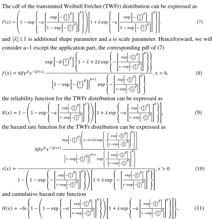
The cdf of the transmuted Weibull Fréchet (TWFr) distribution can be expressed as
𝐹(𝑥) =
( 1 − exp
{ −𝑎 [
exp [− (𝛾
𝑥) 𝛽
]
1 − exp [− (𝛾
𝑥) 𝛽 ] ] 𝑏 })[
1 + 𝜆 exp
{ −𝑎 [
exp [− (𝛾
𝑥) 𝛽
]
1 − exp [− (𝛾
𝑥) 𝛽 ] ] 𝑏 }]
, (7)
and 1 is additional shape parameter and a is scale parameter. Henceforward, we will
consider a=1 except the application part, the corresponding pdf of (7)
𝑓(𝑥) = 𝑏𝛽𝛾𝛽𝑥−(𝛽+1)
exp [−𝑏 (𝛾
𝑥) 𝛽
] {1 − 𝜆 + 2𝜆 exp {− [
exp[−(𝛾 𝑥)
𝛽 ]
1−exp[−(𝛾𝑥)𝛽]
]
𝑏
}}
{1 − exp [− (𝛾
𝑥) 𝛽
]}
𝑏+1
exp {− [
exp[−(𝛾𝑥)𝛽]
1−exp[−(𝛾𝑥)𝛽]
]
𝑏
}
, 𝑥 > 0, (8)
the reliability function for the TWFr distribution can be expressed as
𝑅(𝑥) = 1 − (1 − exp {−𝑎 [
exp[−(𝛾 𝑥)
𝛽 ]
1−exp[−(𝛾𝑥)𝛽]
]
𝑏
}) [1 + 𝜆 exp {−𝑎 [
exp[−(𝛾 𝑥)
𝛽 ]
1−exp[−(𝛾𝑥)𝛽]
]
𝑏
}], (9)
the hazard rate function for the TWFr distribution can be expressed as
𝜏(𝑥) =
𝑏𝛽𝛾𝛽𝑥−(𝛽+1)
exp[−(𝛾𝑥)𝛽]
{
1−𝜆+2𝜆 exp
{ −[
exp[−(𝛾𝑥)𝛽]
1−exp[−(𝛾𝑥)𝛽] ]
𝑏
}}
{1−exp[−(𝛾𝑥)𝛽]} 𝑏+1
exp
{ −[
exp[−(𝛾𝑥)𝛽]
1−exp[−(𝛾𝑥)𝛽] ]
𝑏
}
1 − (1 − exp {− [
exp[−(𝛾𝑥)𝛽]
1−exp[−(𝛾 𝑥) 𝛽 ] ] 𝑏
}) [1 + 𝜆 exp {− [
exp[−(𝛾𝑥)𝛽]
1−exp[−(𝛾 𝑥) 𝛽 ] ] 𝑏 }]
, 𝑥 > 0. (10)
and cumulative hazard rate function
𝐻(𝑥) = −ln {1 − (1 − exp {−𝑎 [
exp[−(𝛾𝑥)𝛽]
1−exp[−(𝛾𝑥)𝛽]
]
𝑏
}) [1 + 𝜆 exp {−𝑎 [
exp[−(𝛾𝑥)𝛽]
1−exp[−(𝛾𝑥)𝛽]
]
𝑏
}]}, (11)
Below is a simple motivation for the development of TWFr distribution. Suppose "𝑇1 and 𝑇2" be two independent random variables from cdf in (7). Define
𝑋 = {𝑇1:2 with probability 1
2(1 + 𝜆); 𝑇2:2 with probability 1
2(1 − 𝜆);
Where 𝑇1:2 = min{𝑇1, 𝑇2} and 𝑇2:2 = max{𝑇1, 𝑇2}, then the cdf of X is given by (7).
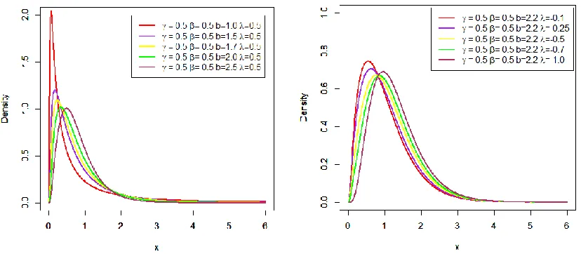
Figure 1: Plots of the TWFr pdf for some parameter values
Figure 2: Plots of the TWFr pdf for some parameter values
3. Mixture Representation
The TWFr density function given in Eq. (8) can be expressed as
𝐹(𝑥; 𝜆, 𝑏, 𝛾, 𝛽) = 1 + (𝜆 − 1) exp
{ − [
exp [− (𝛾
𝑥) 𝛽
]
1 − exp [− (𝛾
𝑥) 𝛽
] ]
𝑏
}
− 𝜆 exp
{ −2 [
exp [− (𝛾
𝑥) 𝛽
]
1 − exp [− (𝛾
𝑥) 𝛽
] ]
𝑏
} , (12)
and after some algebra, we have
𝐹(𝑥) = 1 + ∑ 𝑣𝑖,𝑗
∞
𝑖,𝑗=0
where 𝐻𝑏𝑖+𝑗(𝑥) is the Fr cdf with scale parameter 𝛾[𝑏𝑖 + 𝑗]1 𝛽⁄ and shape parameter β.
𝑣𝑖,𝑗=
(−1)𝑖+𝑗
𝑖! (
−𝛼𝑖
𝑗 ) (𝜆 − 1 − 𝜆 2𝑖),
the corresponding TWFr density function is obtained by differentiating (15)
𝑓(𝑥) = ∑ 𝑣𝑖,𝑗
∞
𝑖,𝑗=0
𝑏𝑏𝑖+𝑗(𝑥), (14)
where ℎ𝑏𝑖+𝑗(𝑥) is the Fr cdf with scale parameter 𝛾[𝑏𝑖 + 𝑗]1 𝛽⁄ and shape parameter β.
Let 𝑐 = inf {𝑥| {exp [− (𝛾 𝑥)
𝛽
]} > 0} . Then the asymptotics of cdf, pdf and hrf as 𝑥 → 𝑐
are given by
𝐹(𝑥)~(1 + 𝜆) exp [− (𝛾
𝑥) 𝛽
] as 𝑥 → 𝑐,
𝑓(𝑥)~𝑏(1 + 𝜆)𝛽𝛾𝛽𝑥−(𝛽+1)exp [− (𝛾 𝑥)
𝛽
] as 𝑥 → 𝑐,
and
ℎ(𝑥)~𝑏(1 + 𝜆)𝛽𝛾𝛽𝑥−(𝛽+1)exp [− (𝛾 𝑥)
𝛽
] as 𝑥 → 𝑐.
The asymptotic of cdf, pdf and hrf when 𝑥 → ∞ are given by
1 − 𝐹(𝑥)~ exp (− {1 − exp [− (𝛾
𝑥) 𝛽
] } −𝑏
) as 𝑥 → ∞,
𝑓(𝑥)~
𝑏𝛽𝛾𝛽𝑥−(𝛽+1)exp [− (𝛾 𝑥)
𝛽 ]
{1 − exp [− (𝛾 𝑥)
𝛽 ] }
𝑏+1 exp (− {1 − exp [− (
𝛾 𝑥)
𝛽 ] }
−𝑏
) as 𝑥 → ∞,
and
ℎ(𝑥)~𝑏𝛽𝛾𝛽𝑥−(𝛽+1)exp [− (𝛾 𝑥)
𝛽
] {1 − exp [− (𝛾 𝑥)
𝛽 ] }
−𝑏−1
as 𝑥 → ∞.
4. Mathematical properties
4.1 Probability weighted moments
The PWMs are expectations of certain functions of a random variable and they can be defined for any random variable whose ordinary moments exist. The PWMs method can generally be used for estimating parameters of a distribution whose inverse form cannot be expressed explicitly. The (𝑠, 𝑟)𝑡ℎ PWMs of X following the TWFr model, say 𝜌𝑠,𝑟 is
formally defined by
𝜌𝑠,𝑟 = 𝐸{𝑋𝑠𝐹(𝑋)𝑟} = ∫ 𝑥∞ 𝑠𝐹(𝑥)𝑟𝑓(𝑥)𝑑𝑥. −∞
Using equations (pdf) and (cdf), we can write
where ℎ𝑏(𝑖+1)+𝑗(𝑥) is the Fr density with scale parameter 𝛾[𝑏(𝑖 + 1) + 𝑗]1 𝛽⁄ and shape
parameter β. and
𝑝𝑖,𝑗= ∑
(−1)𝑘+ℎ+𝑖+𝑗(ℎ + 1)𝑖[(1 + 𝜆) (𝑟 + 𝑘
ℎ ) − 2𝜆 (
𝑟 + 𝑘 + 1 ℎ )] 𝑖! 𝑏−1𝜆−𝑘(1 + 𝜆)𝑘−𝑟[𝑏(𝑖 + 1) + 𝑗]
∞
𝑘,ℎ=0
(𝑘𝑟) (−[𝑏(𝑖 + 1) + 1]𝑗 ).
Then, the (𝑠, 𝑟)𝑡ℎ PWMs of X can be expressed as
𝜌𝑠,𝑟 = ∑
𝑝𝑖,𝑗 𝛾−𝑟 ∞
𝑖,𝑗=0
[𝑏(𝑖 + 1) + 𝑗] 𝑟
𝛽 Г (1 −𝑟 𝛽).
4.2 Moments, incomplete moments and generating function
The rth ordinary moment of X is given by 𝜇𝑟′ = 𝐸(𝑋𝑟) = ∫∞ 𝑥𝑟𝑓(𝑥)𝑑𝑥.
−∞ Then we obtain
𝜇𝑟′ = ∑ 𝑣𝑖,𝑗 𝛾−𝑟 ∞
𝑖,𝑗=0
[𝑎𝑖 + 𝑗] 𝑟
𝛽 Г (1 −𝑟
𝛽). (15)
Setting 𝑟 = 1, we have the mean of X. The last integration can be computed numerically for most parent distributions. The skewness and kurtosis measures can be calculated from the ordinary moments using well-known relationships. Then nth central moments of X,
say 𝑀𝑛, follows as 𝑀𝑛 = 𝐸(𝑋 − 𝜇)𝑛 = ∑ (−1)ℎ(𝑛
ℎ) (𝜇1′)𝑛𝜇𝑛−ℎ′ 𝑛
ℎ=0 . The cumulants (𝑘𝑛)
of X follow recursively from 𝑘𝑛 = 𝜇𝑛′ − ∑ (−1)ℎ(𝑛 − 1
𝑟 − 1) 𝑘𝑟𝜇𝑛−ℎ ′ , 𝑛−1
𝑟=0 where 𝑘1 =
𝜇1′, 𝑘
2 = 𝜇2′ − 𝜇1′ 2, 𝑘3 = 𝜇3′ − 3𝜇2′𝜇1′ + 𝜇1′ 3, etc. The skewness and kurtosis measures
also can be calculated from the ordinary moments using well-known relationships. The main applications of the first incomplete moments refer to the mean deviations and Bonferroni and Lorenz curves. These curves are very useful in economics, reliability, demography, insurance and medicine. The rth incomplete moment, say 𝜑𝑟(𝑡), of X can
be expressed from (10) as
𝜑𝑟(𝑡) = ∫ 𝑥𝑡 𝑟𝑓(𝑥)𝑑𝑥 −∞
= ∑ 𝑣𝑖,𝑗
𝛾−𝑟 ∞
𝑖,𝑗=0
[𝑎𝑖 + 𝑗] 𝑟
𝛽 Г (1 − 𝑟
𝛽, [𝑎𝑖 + 𝑗]− ( 𝛾 𝑡)
𝛽
). (16)
The mean deviations about the mean [𝛿1 = 𝐸(|𝑋 − 𝜇1′|)] and about the median [𝛿2 =
𝐸(|𝑋 − 𝑀|)] of X are given by 𝛿1 = 2𝜇1′𝐹(𝜇
1′) − 2𝜑1(𝜇1′) and 𝛿2 = 𝜇1′ − 2𝜑1(𝑀),respectively, where 𝜇1′ = 𝐸(𝑋), 𝑀 = 𝑚𝑒𝑑𝑖𝑎𝑛(𝑋) = 𝑄(0.5) is the median, 𝐹(𝜇1′) is easily calculated from (5) and 𝜑
1(𝑡) is the first incomplete moment given by
(12) with r=1. Here, we provide two formulae for the moment generating function (mgf)
𝑀𝑥(𝑡) = 𝐸(𝑒𝑡𝑋) of X. Clearly, the first one can be derived from equation (9), for 𝑟 < 𝑏,
as
𝑀𝑥(𝑡) = ∑∞𝑘=0𝛶𝑘𝑀[(𝛼+𝑘)𝜃](𝑡) = ∑∞𝑘=0𝛶𝑘∑ 𝑡𝑟 𝑟! ∞
𝑟=0 𝜇𝑟′ = ∑
𝛶𝑘 𝑡𝑟 𝑎−𝑟𝑟! ∞
𝑘,𝑟=0 [(𝛼 + 𝑘)𝜃] 𝑟
A second formula for 𝑀𝑥(𝑡). Setting 𝑦 = 𝑥−1 in (3), we can write this mgf 𝑀(𝑡; 𝑎, 𝑏) = 𝑏𝑎𝑏∫ exp (𝑡
𝑦) ∞
0 𝑦
(𝑏−1)exp{−(𝑎𝑦)𝑏}. By expanding the first exponential and calculating
the integral, we have
𝑀(𝑡; 𝛾, 𝛽) = 𝑏𝛾𝑏∫ ∑𝑡
𝑚
𝑚! ∞
𝑚=0 ∞
0
exp (𝑡 𝑦) 𝑦
𝛽−𝑚−1exp{−(𝛾𝑦)𝛽} = ∑ 𝛾𝑚 𝑡𝑚 𝑚! ∞
𝑚=0
Г (𝛽 − 𝑟
𝛽 ),
where the gamma function is well-defined for any non-integer b. Consider the Wright generalized hypergeometric function defined by
𝑝𝛹𝑞[
(𝛼1, 𝐴1), … , (𝛼1, 𝐴𝑝) (𝛽1, 𝐵1), … , (𝛽1, 𝐵𝑝)
; 𝑥] = ∑∏ Г(𝛼𝑗+ 𝐴𝑗𝑛)
𝑝 𝑗=1
∏𝑞𝑗=1Г(𝛽𝑗+ 𝐵𝑗𝑛) ∞
𝑛=0
𝑥𝑛 𝑛!
Then, we can write 𝑀(𝑡; 𝛾, 𝛽) as
𝑀(𝑡; 𝛾, 𝛽) = 1𝛹0[(1 − 𝛽 −1)
− ; 𝛾𝑡]. (17)
Combining expressions (17) and the above equation, we obtain the mgf of X, say 𝑀(𝑡), as
𝑀(𝑡; 𝛾, 𝛽) = ∑ 𝑣𝑖,𝑗 ∞
𝑖,𝑗=0
1𝛹0[((1 − 𝛽 −1)
− ; 𝛾[𝑏𝑖 + 𝑗]
1 𝛽𝑡].
4.3 Order statistics
Let 𝑋1, 𝑋2, … , 𝑋𝑛 be random sample from the TWFr model of distributions and let 𝑋1:𝑛, 𝑋2:𝑛, … , 𝑋𝑛:𝑛be the corresponding order statistics. The pdf of ith order statistics, say 𝑋𝑖:𝑛, can be written as
𝑓𝑖:𝑛(𝑥) = 𝑓(𝑥)
𝐵(𝑖,𝑛−𝑖+1)∑ (−1)
𝑗(𝑛 − 𝑖
𝑗 )
𝑛−𝑖
𝑗=0 𝐹𝑗+𝑖−1(𝑥),
where 𝐵(. , . ) is the beta function. Substituting (5) and (6) in equation (13) and using a power series expansion, we get
𝑡𝑚,𝑤= ∑
(−1)𝑘+ℎ+𝑚+𝑤[(1 + 𝜆) (𝑗 + 𝑖 + 𝑘 − 1
ℎ ) − 2𝜆 (
𝑗 + 𝑖 + 𝑘
ℎ )]
𝑖! 𝑏−1 𝜆−𝑘(ℎ + 1)−𝑚(1 + 𝜆)𝑘−(𝑗+𝑖−1)[𝑏(𝑚 + 1) + 𝑤]
∞
𝑘,ℎ=0
(𝑗 + 𝑖 − 1
𝑘 ) (
−[𝑏(𝑚 + 1) + 1]
𝑤 ).
The pdf of 𝑋𝑖: 𝑛 can be expressed as
𝑓𝑖:𝑛(𝑥) = ∑
(−1)𝑗(𝑛 − 𝑖
𝑗 )
𝐵(𝑖, 𝑛 − 𝑖 + 1) 𝑛−𝑖
𝑗=0
∑ 𝑡𝑚,𝑤ℎ𝑏(𝑚+1)+𝑤 𝑛−𝑖
𝑗=0
(𝑥).
Where ℎ𝑏(𝑚+1)+𝑤(𝑥) is the Fr density with scale parameter 𝛾[𝑏(𝑚 + 1) + 𝑤] 1
𝛽 and shape
parameter β. Based on the last equation, we note that the properties of 𝑋𝑖: 𝑛 follow from those properties of 𝑌𝑘+1. For example, the moments of 𝑋𝑖: 𝑛 can be expressed as
𝐸(𝑋𝑖:𝑛𝑞 ) = ∑ ∑
(−1)𝑗(𝑛 − 𝑖 𝑗 ) 𝑡𝑚,𝑤 𝐵(𝑖, 𝑛 − 𝑖 + 1)𝛾−𝑞 𝑛−𝑖
𝑗=0 ∞
𝑚,𝑤=0
[𝑏(𝑚 + 1) + 𝑤] 𝑞
𝛽Г (1 −𝑞
The L-moments are analogous to the ordinary moments but can be estimated by linear combinations of order statistics. They exist whenever the mean of the distribution exists, even though some higher moments may not exist, and are relatively robust to the effects of outliers. Based upon the moments in equation (18), we can derive explicit expressions for the L-moments of X as infinite weighted linear combinations of the means of suitable TWFr order statistics. They are linear functions of expected order statistics defined by
𝜆𝑟 = 1
𝑟∑(−1)
𝑑 𝑟−1
𝑑=0
(𝑟 − 1
𝑑 ) 𝐸(𝑋𝑟−𝑑:𝑟), 𝑟 ≥ 1.
4.4 Moments of the residual and reversed residual life
Let X be a random variable usually representing the life length for a certain unit at age t (where this unit can have multiple interpretations), then the random variable 𝑋𝑡= 𝑋 − 𝑡|𝑋 > 𝑡 represents the remaining lifetime beyond that age. Moreover, the nth moment of the residual life, denoted by
𝑚𝑛(𝑥) = 𝐸{(𝑋 − 𝑥)𝑛|𝑋 > 𝑥}, 𝑛 = 1, 2, … uniquely determines F(x), The nth moment of
the residual life of X is given by 𝑀𝑛(𝑡) = 1
1−𝐹(𝑡)∫ (𝑥 − 𝑡)
𝑛𝑑𝐹(𝑥). ∞
𝑡 Then, we ca write
(for 𝑟 < 𝛽 ) 𝑚𝑛(𝑡) =
1 1−𝐹(𝑡)∑
(−1)𝑛−𝑟𝑡𝑛−𝑟𝑛! 𝑟!Г(𝑛−𝑟+1) 𝑛
𝑟=0 ∑
𝑣𝑖,𝑗 𝛾−𝑟 ∞
𝑖,𝑗=0 (𝑏𝑖 + 𝑗) 𝑟
𝛽Г (1 −𝑟
𝛽, (𝑏𝑖 + 𝑗) ( 𝛾 𝑡)
𝛽 ).
The nth moment of the reversed residual life, say 𝑀𝑛(𝑡) = 𝐸{(𝑡 − 𝑋)𝑛|𝑋 ≤ 𝑡} for 𝑡 > 0
and 𝑛 = 1, 2, … uniquely determines F(x) (Navarro et al. 1998). We obtain 𝑀𝑛(𝑡) = 1
𝐹(𝑡)∫ (𝑡 − 𝑥)
𝑛𝑑𝐹(𝑥). 𝑡
0 Therefore, the nth moment of the reversed residual life of X given
that 𝑟 < 𝛽 becomes
𝑀𝑛(𝑡) = 1
𝐹(𝑡)∑
(−1)𝑗𝑛! 𝑟! (𝑛 − 𝑟)! 𝑛
𝑟=0
∑ 𝑣𝑖,𝑗
𝛾−𝑟 ∞
𝑖,𝑗=0
(𝑏𝑖 + 𝑗) 𝑟
𝛽Г (1 −𝑟
𝛽, (𝑏𝑖 + 𝑗) ( 𝛾 𝑡)
𝛽 ).
The mean inactivity time (MIT) or mean waiting time (MWT) also called the mean reversed residual life function is defined by 𝑀1(𝑡) = 𝐸{(𝑡 − 𝑋)|𝑋 ≤ 𝑡}, and it represents the waiting time elapsed since the failure of an item on condition that this failure had occurred in (0; x). The MRRL of X can be obtained by setting n = 1 in the above equation.
4.5 Stress-strength model
random variables with 𝑇𝑊𝐹𝑟(𝜆1, 𝑏1, 𝛾, 𝛽) and 𝑇𝑊𝐹𝑟(𝜆2, 𝑏2, 𝛾, 𝛽) distributions. The reliability is defined by 𝑅 = ∫ 𝑓1(𝑥, 𝜆1, 𝑏1, 𝛾, 𝛽)𝐹2(𝑥, 𝜆2, 𝑏2, 𝛾, 𝛽)
∞
0 𝑑𝑥. Then, we can
write
𝑹 = ∑ 𝑎𝑖,𝑗
∞
𝑖,𝑗=0
∫ ℎ𝑏1𝑖+𝑗(𝑥)𝑑𝑥
∞
0 +
∑ 𝑏𝑖,𝑗,𝑘,ℎ ∞
𝑖,𝑗,ℎ,𝑘=0
∫ ℎ𝑏1𝑖+𝑗+𝑏1ℎ+𝑘(𝑥)𝑑𝑥 ∞
0
Where
𝑎𝑖,𝑗 =
(−1)𝑖+𝑗
𝑖! (
−𝑏1𝑖
𝑗 ) (𝜆1− 1 − 𝜆1 2𝑖)
And
𝑏𝑖,𝑗,𝑘,ℎ =
(−1)𝑖+𝑗+ℎ+𝑘(𝜆
1− 1 − 𝜆1 2𝑖) ( −𝑏1𝑖
𝑗 ) (
−𝑏2𝑖
𝑘 )
𝑖! (𝑏1𝑖 + 𝑗)[𝑏1𝑖 + 𝑗 + 𝑏2ℎ + 𝑘](𝜆1− 1 − 𝜆1 2ℎ)−1
Thus, the reliability, R, can be expressed as
𝑅 = ∑ 𝑎𝑖,𝑗
∞
𝑖,𝑗=0
+ ∑ 𝑏𝑖,𝑗,𝑘,ℎ ∞
𝑖,𝑗,ℎ,𝑘=0
.
4.6 Quantile Function
The quantile function (qf) of X, where 𝑋 − 𝑇𝑊𝐹𝑟(𝛾, 𝛽, 𝑎, 𝑏, 𝜆) is obtained by inverting
𝑋𝑈 = 𝐹−1(𝑈) as
𝑋𝑈 = 𝛾 (− log [1 − log {1 −(1 + 𝜆) − √(1 + 𝜆
2) − 4𝜆𝑈
2𝜆 }
−1 𝑏
]) −1
𝛽
.
Simulating the TWFr random sample is straightforward. If U is a uniform variate on the unit interval (0, 1) then the random variable X follows Eq. (8).
Particularly, the distribution median is
𝑋0.5 = 𝛾 (− log [1 −1
𝑎log {1 −
(1+𝜆)−√(1+𝜆2)−4𝜆0.5
2𝜆 }
−1 𝑏
]) −𝛽1
,
then
𝑋0.5 = 𝛾 (− log [1 −1 𝑎log {
(𝜆 − 1) + √(1 + 𝜆2)
2𝜆 }
−1𝑏
]) −1𝛽
.
5. Maximum Likelihood Estimation
𝐿 = n ln(𝑎𝑏𝛽𝛼𝛽) − (𝛽 + 1) ∑ ln(𝑥𝑖) 𝑛
𝑖=1
+ ∑ ln
{
1 − 𝜆 + 2𝜆 exp
{ − [
exp [− (𝛾
𝑥𝑖) 𝛽
]
1 − exp [− (𝛾
𝑥𝑖) 𝛽 ] ] 𝑏 }} 𝑛 𝑖=1
− (𝑏 + 1) ∑ ln {1 − exp [− (𝛾
𝑥𝑖 ) 𝛽 ]} 𝑛 𝑖=1
+ ∑ ln
{ exp
{ − [
exp [− (𝛾
𝑥𝑖) 𝛽
]
1 − exp [− (𝛾
𝑥𝑖) 𝛽 ] ] 𝑏 }} 𝑛 𝑖=1
Differentiate log-likelihood function with respect to parameters.
𝜕𝐿 𝜕𝑏=
𝑛
𝑏+ 𝛽 log 𝛾 − ∑
2𝜆 exp {− [
exp[−(𝛾 𝑥𝑖) 𝛽 ] 1−exp[−(𝛾 𝑥𝑖) 𝛽 ] ] 𝑏 } [ exp[−(𝛾 𝑥𝑖) 𝛽 ] 1−exp[−(𝛾 𝑥𝑖) 𝛽 ] ] 𝑏 log 𝑏
{1 − 𝜆 + 2𝜆 exp {− [
exp[−(𝛾 𝑥𝑖) 𝛽 ] 1−exp[−(𝛾 𝑥𝑖) 𝛽 ] ] 𝑏 }} 𝑛 𝑖=1
− ∑ log {1 − exp [− (𝛾 𝑥𝑖 )
𝛽
]} + ∑ [
exp [− (𝛾 𝑥𝑖)
𝛽 ]
1 − exp [− (𝑥𝛾 𝑖) 𝛽 ] ] 𝑏 log 𝑏 𝑛 𝑖=1 𝜕𝐿 𝜕𝛽= 𝑛
𝛽+ 𝑏 log 𝛾 − ∑ log 𝑥𝑖
𝑛 𝑖=1 − ∑ (𝛾 𝑥𝑖 ) 𝛽 log 𝛽 𝑛 𝑖=1 + ∑
2𝑏𝜆 exp {− [
exp[−(𝛾 𝑥𝑖) 𝛽 ] 1−exp[−(𝛾 𝑥𝑖) 𝛽 ] ] 𝑏 } [ exp[−(𝛾 𝑥𝑖) 𝛽 ] 1−exp[−(𝛾 𝑥𝑖) 𝛽 ] ] 𝑏−1
exp [− (𝛾
𝑥𝑖) 𝛽 ] (𝛾 𝑥𝑖) 𝛽 log 𝛽
{1 − 𝜆 + 2𝜆 exp {− [
exp[−(𝛾 𝑥𝑖) 𝛽 ] 1−exp[−(𝛾 𝑥𝑖) 𝛽 ] ] 𝑏
}} [1 − exp [− (𝛾
𝑥𝑖) 𝛽 ]] 2 𝑛 𝑖=1 − ∑
(𝑏 + 1) exp [− (𝛾
𝑥𝑖) 𝛽 ] (𝛾 𝑥𝑖) 𝛽 log 𝛽
{1 − exp [− (𝛾
𝑥𝑖) 𝛽 ]} 𝑛 𝑖=1 − 𝑏 ∑
exp [− (𝛾
𝑥𝑖) 𝛽 ] (𝛾 𝑥𝑖) 𝛽 log 𝛽
[1 − exp [− (𝛾
𝑥𝑖) 𝛽 ]] 2 𝑛 𝑖=1 𝜕𝐿 𝜕𝛾= 𝑛𝑏𝛽 𝛾 − 𝛽 ∑ ( 𝛾 𝑥𝑖) 𝛽−1 1 𝑥𝑖 𝑛 𝑖=1 + ∑
2𝑏𝜆 exp {− [
exp[−(𝛾 𝑥𝑖) 𝛽 ] 1−exp[−(𝛾 𝑥𝑖) 𝛽 ] ] 𝑏 } [ exp[−(𝛾 𝑥𝑖) 𝛽 ] 1−exp[−(𝛾 𝑥𝑖) 𝛽 ] ] 𝑏−1
𝛽 exp[−(𝛾 𝑥𝑖) 𝛽 ](𝛾 𝑥𝑖) 𝛽−11 𝑥𝑖 [1−exp[−(𝛾 𝑥𝑖) 𝛽 ]] 2
{1 − 𝜆 + 2𝜆 exp {− [
exp[−(𝛾 𝑥𝑖) 𝛽 ] 1−exp[−(𝛾 𝑥𝑖) 𝛽 ] ] 𝑏 }} 𝑛 𝑖=1
− (𝑏 + 1) ∑
𝛽 exp [− (𝑥𝛾
𝑖) 𝛽 ] (𝑥𝛾 𝑖) 𝛽−1 1 𝑥𝑖
{1 − exp [− (𝛾
𝑥𝑖) 𝛽 ]} 𝑛 𝑖=1 + 𝑏 ∑ [
exp [− (𝑥𝛾
𝑖) 𝛽
]
1 − exp [− (𝑥𝛾
𝑖) 𝛽
] ]
𝑏−1
𝛽 exp [− (𝑥𝛾
𝑖) 𝛽 ] (𝑥𝛾 𝑖) 𝛽−1 1 𝑥𝑖
[1 − exp [− (𝑥𝛾
𝜕𝐿
𝜕𝜆= ∑
2 exp {− [
exp[−(𝛾 𝑥𝑖)
𝛽 ]
1−exp[−(𝛾 𝑥𝑖)
𝛽 ]
]
𝑏
} − 1
{1 − 𝜆 + 2𝜆 exp {− [
exp[−(𝛾 𝑥𝑖)
𝛽 ]
1−exp[−(𝛾 𝑥𝑖)
𝛽 ]
]
𝑏
}}
𝑛
𝑖=1
6. Applications
In this section, we provide two real dataset applications to illustrate the importance of the TWFr distribution. The MLEs of the parameters for these models are calculated and four goodness-of-fit statistics are used to compare the new family with its sub-models. The first data set represents the carbon fibers of 66 observations. The data are: 0.39, 0.85, 1.08, 1.25, 1.47, 1.57, 1.61, 1.61, 1.69, 1.8, 1.84, 1.87, 1.89, 2.03, 2.03, 2.05, 2.12, 2.35, 2.41, 2.43, 2.48, 2.5, 2.53, 2.55, 2.55, 2.56, 2.59, 2.67, 2.73, 2.74, 2.79, 2.81, 2.82, 2.85, 2.87, 2.88, 2.93, 2.95, 2.96, 2.97, 3.09, 3.11, 3.11, 3.15, 3.15, 3.19, 3.22, 3.22, 3.27, 3.28, 3.31, 3.31, 3.33, 3.39, 3.39, 3.56, 3.6, 3.65, 3.68, 3.7, 3.75, 4.2, 4.38, 4.42, 4.7, 4.9.
The second data set consists of 63 observations of the strengths of 1.5 cm glass fibers, originally obtained by workers at the UK National Physical Laboratory. The data are: 0.55, 0.93, 1.25, 1.36, 1.49, 1.52, 1.58, 1.61, 1.64, 1.68, 1.73, 1.81, 2, 0.74, 1.04, 1.27, 1.39, 1.49, 1.53, 1.59, 1.61, 1.66, 1.68, 1.76, 1.82, 2.01, 0.77, 1.11, 1.28, 1.42, 1.5, 1.54, 1.6, 1.62, 1.66, 1.69, 1.76, 1.84, 2.24, 0.81, 1.13, 1.29, 1.48, 1.5, 1.55, 1.61, 1.62, 1.66, 1.7, 1.77, 1.84, 0.84, 1.24, 1.3, 1.48, 1.51, 1.55, 1.61, 1.63, 1.67, 1.7, 1.78, 1.89. These data have also been analyzed by Smith and Naylor (1987).
The MLEs are computed using Mathematica. The goodness of fit measures, including the Akaike information criterion (AIC), Bayesian information criterion (BIC), Anderson-Darling (A∗), Cramér–von Mises (W∗) statistics are computed to compare the fitted
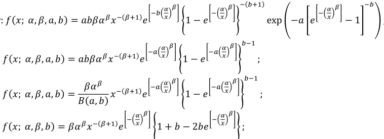
models. Generally the small values of these measures indicate the better the fit to the data. These goodness of fit measures are also computed using Mathematica. We compare the proposed model TWFr, with Kumaraswamy Fréchet (KFr) (Mead, 2014), beta Fréchet (BFr) (Nadarajah & Gupta, 2004), transmuted Fréchet (Mahmoud & Mandouh, 2013), Weibull Fréchet (WFr) (Afify et al. 2016). Their density functions (for x>0) are given by:
WFr: 𝑓(𝑥; 𝛼, 𝛽, 𝑎, 𝑏) = 𝑎𝑏𝛽𝛼𝛽𝑥−(𝛽+1)𝑒[−𝑏(
𝛼 𝑥)
𝛽 ]
{1 − 𝑒[−(
𝛼 𝑥)
𝛽 ]
}
−(𝑏+1)
exp (−𝑎 [𝑒[−(
𝛼 𝑥)
𝛽 ]
− 1]
−𝑏
) ;
KFr: 𝑓(𝑥; 𝛼, 𝛽, 𝑎, 𝑏) = 𝑎𝑏𝛽𝛼𝛽𝑥−(𝛽+1)𝑒[−𝑎(
𝛼 𝑥)
𝛽 ]
{1 − 𝑒[−𝑎(
𝛼 𝑥)
𝛽 ]
}
𝑏−1
;
BFr: 𝑓(𝑥; 𝛼, 𝛽, 𝑎, 𝑏) = 𝛽𝛼
𝛽
𝐵(𝑎, 𝑏)𝑥
−(𝛽+1)𝑒[−𝑎( 𝛼 𝑥)
𝛽 ]
{1 − 𝑒[−𝑎(
𝛼 𝑥)
𝛽 ]
}
𝑏−1
;
TFr: 𝑓(𝑥; 𝛼, 𝛽, 𝑏) = 𝛽𝛼𝛽𝑥−(𝛽+1)𝑒[−(
𝛼 𝑥)
𝛽 ]
{1 + 𝑏 − 2𝑏𝑒[−(
𝛼 𝑥)
𝛽 ]
} ;
Table-1: MLEs and goodness of fit measures for data set 1
Parameters Probability Distributions
KFr BFr TFr WFr TWFr
α 9.4E+09 522.623 3.53178 0.04630291 1.5069E-05
β 0.12847 0.45492 1.23875 0.674984 0.160797
λ - - - - -0.646467
a 1.57844 0.52752 - 1.8525E-06 3.0372E-14
b 2.3E+11 14732.9 2.45 4.72167 16.6086
Log( likelihood) -86.6727 -87.6214 -90.7381396 -86.2841 -85.35918
A∗ 0.57577 0.78347 10.0076 0.623812 0.422544
W∗ 0.1028 0.14884 2.54272 0.118206 0.0704867
AIC 181.543 183.243 187.476 180.68 180.284
BIC 190.104 192.1 194.045 189.327 191.132
Table-2: MLEs and goodness of fit measures for data set 2
Parameters
Probability distributions
KFr BFr EFr TFr WFr TWFr
α 2.605E-07 185850000 8.44175 1.0937 0.3865 0.000112174
β 0.481855 0.164219 0.954717 3.22166 0.2436 0.034959799
λ - - - -0.77447 - -0.502657301
a 20998 1.93339 132.827 - 1.4762 130.0266213
b 73124.2 2976000000 - 16.8561 105.0252683
Log( likelihood) -17.6651 -18.6831 -21.999 -43.1516 -15.5005 -14.3672112
A∗ 1.81873 2.17081 2.79072 6.0437 1.34103 1.05787
W∗ 0.313038 0.403759 0.510634 1.10797 0.232647 0.17196
AIC 43.3301 45.3661 49.9972 92.3031 39.0011 38.7344
(a) (b)
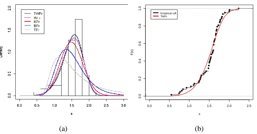
Fig. 1: Plots of the estimated (a) pdfs and (b) cdf for the TWFr and their sub-models for first dataset-1.
(a) (b)
Fig. 2: Plots of the estimated (a) pdfs and (b) cdf for the TWFr and their sub-models for first dataset-2.
Conclusion
There has been a growing interest among statisticians and applied researchers in developing flexible lifetime models for the betterment of modeling survival data. In this paper, we introduce a new four-parameter extreme value model called the Transmuted Weibull Fréchet (TWFr) distribution, which extends the Fréchet (Fr) distribution. An obvious reason for generalizing Fr distribution is the fact that the generalization provides
0.0 0.5 1.0 1.5 2.0 2.5
0
.0
0
.2
0
.4
0
.6
0
.8
1
.0
Empirical Cumulative Distribution Plot
x
F
(x)
more flexibility to analyze real life data. We study some of its statistical and mathematical properties. The TWFr density function can be expressed as a linear mixture of Fr densities. We derive explicit expressions for the ordinary and incomplete moments mean deviations, generating function, moments of the residual and reversed residual life. We also obtain the density function of the order statistics and their moments. We estimate the model parameters by maximum likelihood method. The new distribution applied to two real data sets provide better fits than some other related non-nested models. We hope that the proposed model will attract wider applications in areas such as engineering, survival and lifetime data, meteorology, hydrology, economics (income inequality) and others.
References
1. Afify, A. Z., Hamedani, G. G. Ghosh, I. and Mead, M. E. (2015). The transmuted Marshall–OlkinFréchetdistribution: properties and applications. Int. J. Statist. Probab., 4, 132–184.
2. Afify, A. Z., Yousof, H. M., Cordeiro, G.M. and Ahmad, M. (2016a). The Kumaraswamy Marshall-Olkin Fréchet distribution with applications. Journal of ISOSS, 2, 1-18.
3. Afify, A. Z., Yousof, H. M., Cordeiro, G. M., Ortega, E. M. M. and Nofal, Z. M. (2016b). The Weibull Fréchet distribution and its applications. Journal of Applied Statistics, 43, 2608–2626.
4. Afify, A. Z., Yousof, H. M. and Nadarajah, S. (2016c). The beta transmuted-H family of distributions: properties and applications. Stasistics and its Inference, forthcoming.
5. Batchelor, J. R. and Hackett, M. (1970). HL-A matching in treatment of burned patients with skin allografts. The Lancet, 296, 581-583.
6. Battjes, J. A. (1978). Probabilistic aspects of ocean waves. Technical Report 77-2, Laboratory of fluid mechanics, Department of civil engineering, Delft University of Technology.
7. Barreto-Souza, W. M., Cordeiro, G. M. and Simas, A. B. (2011). Some results for beta Fréchet distribution. Commun. Statist. Theory-Meth., 40, 798-811.
8. Borgman, L. E. (1063). Risk criteria. Journal of the Waterways and Harbors Division, ASCE, 89, 1–35.
9. Borgman, L. E. (1970). Maximum wave height probabilities for a random number of random intensity storms. Technical report, University of California. Hydraulic Engineering Laboratory.
10. Borgman, L. E. (1973). Probabilities for highest wave in hurricane. Journal of the Waterways, Harbors and Coastal Engineering Division, 99, 85–207.
11. Bryant, P. J. (1983). Cyclic gravity waves in deep water. The Journal of the Australian Mathematical Society. Series B. Applied Mathematics, 25, 2–15. 12. Castillo, E. and Sarabia, J. M. (1992). Engineering analysis of extreme value data:
13. Castillo, E. and Sarabia, J. M. (1994). Extreme value analysis of wave heights. Journal of Research of the National Institute of Standards and Technology, 99, 445–454.
14. Cavanie, A. Arhan, X. and Ezraty. X. (1976). A statistical relationship between individual heights and periods of storm waves. Behaviour of off-shore structures. 15. Chakrabarti, S. K. and Cooley, R. P. (1977). Ocean wave statistics for 1961 north
atlantic storm. Journal of the Waterway Port Coastal and Ocean Division, 103, 433–448.
16. Cordeiro, G. M., Nadarajah, S., Ortega. E. M. M. and Ramires, T. G. (2016). An alternative two-parameter gamma generated family of distributions: properties and applications. Hacettepe Journal of Mathematics and Statistics, forthcoming. 17. Cordeiro, G. M., Ortega, E. M. M. and Ramires, T. G. (2015). A new generalized
Weibull family of distributions: mathematical properties and applications. Journal of Statistical Distributions and Applications, 2, 1–25.
18. Court, A. (1953). Wind extremes as design factors. Journal of the Franklin Institute, 256, 39 – 56.
19. Draper, L. (1963). Derivation of a design wave from instrumental records of sea waves. In ICE Proceedings, pages 291–304. Ice Virtual Library.
20. Earle, M. D., Ebbesmeyer, C. C. and Evans, D.J. (1974). Height-period joint probabilities in hurricane camille. Journal of the Waterways, Harbors and Coastal Engineering Division, 100, 257–264.
21. Elbatal, I. Asha, G. and Raja, V. (2014). Transmuted exponentiated Fréchet distribution: properties and applications. J. Stat. Appl. Pro., 3, 379-394.
22. Fisher, R. A. and Tippett, L. H. C. (1928). Limiting forms of the frequency distribution of the largest or smallest member of a sample. In Mathematical Proceedings. of the Cambridge Philosophical Society, pages 180–190. Cambridge Univ Press.
23. Ferro, C. A. T. and Segers, J. (2003). Inference for clusters of extreme values. Journal of the Royal Statistical Society: Series B (Statistical Methodology), 65, 545–556.
24. Fr´echet, M. (1927). Sur la loi de probabilit´e de l´ecart maximum. Ann. de la Soc. polonaisede Math, 6, 93–116.
25. Gnedenko, B. (1943). Sur la distribution limite du terme maximum d’une serie aleatoire. Annals of Mathematics, Volume 44.
26. Goodknight, R. C. and Russell, T. L. (1963) Investigation of the statistics of wave heights. ASCE Journal of the Waterways and Harbors Division, 89, 29–52.
27. Hamedani, G. G. (2013). On certain generalized gamma convolution distributions II, Technical Report, No. 484, MSCS, Marquette University.
28. Harlow, D. G. (2002). Applications of the Fréchet distribution function, Int. J. Mater. Prod. Technol, 17, 482–495.
29. Kotz, S. and Johnson, N. L. (1992). Breakthroughs in Statistics: Foundations and basic theory. Springer, Volume 1.
31. Krishna, E., Jose, K. K., Alice, T. and Risti, M. M. (2013). The Marshall Olkin Fréchetdistribution. Communications in Statistics-Theory and Methods, 42, 4091- 4107.
32. Leadbetter, M. R., Lindgren, G. and Rootz´en, H. (1983). Extremes and related properties of random sequences and processes. Springer Verlag, Volume 11. 33. Mahmoud, M. R. and Mandouh, R. M. (2013). On the transmuted Fréchet
distribution. Journal of Applied Sciences Research, 9, 5553-5561.
34. Nadarajah, S. and Gupta, A. K. (2004). The beta Fréchet distribution. Far East Journal of Theoretical Statistics, 14, 15-24.
35. Nadarajah, S. and Kotz, S. (2003). Moments of some J-shaped distributions. Journal of Applied Statistics, 30, 311-317.
36. Nadarajah, S. and Kotz, S. (2003). The exponentiated exponential distribution.
Available online at http://interstat.stat
journals.net/YEAR/2003/abstracts/0312001.php/
37. Nadarajah, S. and Kotz, S. (2008). Sociological models based onFréchetrandom variables, Qual Quant, 42, 89–95.
38. Ramires, T. G., Ortega, E. M. M., Cordeiro, G. M. and Hamedani, G. G. (2013). The beta generalized half-normal geometric distribution. Studia Scientiarum Mathematicarum Hungarica, 50, 523–554.
39. Von Mises, R. (1964). Selected papers of Richard von Mises, American mathematical society, Volume 1.
40. Yousof, H. M., Afify, A. Z., Alizadeh, M., Butt, N. S., Hamedani, G. G. and Ali, M. M. (2015). The transmuted exponentiated generalized-G family of distributions. Pak. J. Stat. Oper. Res., 11, 441-464.
41. Yousof, H. M., Afify, A. Z., Ebraheim, A. N., Hamedani, G. G. and Butt, N. S. (2016). On six-parameterFréchetdistribution: properties and applications, Pak. J. Stat. Oper. Res., 12, 281-299.
42. Zaharim, A., Najid, S.K., Razali, A.M. and Sopian, K. (2009). Analyzing Malaysian wind speed data using statistical distribution, Proceedings of the 4th IASME/WSEAS International Conference on Energy and Environment, Cambridge.
43. Zghoul, A. A. (2011). Record values from a family of J-shaped distributions. Statistics, 71, 355-365.