Ali H. Abuzaid
Department of Mathematics, Faculty of Science, Al Azhar University – Gaza, Palestine [email protected]
Walaa A. Abu El-laban
Department of Applied Statistics, Faculty of Economic and Administrative Sciences Al Azhar University – Gaza, Palestine
Abdul Ghapor Hussin
Department of Defence Science, Faculty of Defence Science and Technology National Defence University of Malaysia, Malaysia
Abstract
This paper extends the simple linear regression model with wrapped Cauchy error to the functional case when both variables are subjected to wrapped Cauchy errors. Assuming the ratio between the two error variances is known and the slope parameter equals one the maximum likelihood estimates are obtained. The closed-form expression for the maximum likelihood estimators are not available and the estimates are obtained iteratively by choosing a suitable initial values. The quality of estimates and the accuracy of the model are illustrated via simulations and the results revealed an acceptable performance of the estimators where they are unbiased, consistent and robust. The sampling variances of the model parameters are obtained via bootstrapping methods and consequently the confidence intervals were constructed. The proposed model is illustrated with an application on the analysis of wind directions data at two cities in the Gaza strip, Palestine.
Keywords: Bootstrap, EIVM, robustness, Wind direction.
1. Introduction
The functional relationship model is a part of the general class of Error-In-Variables Models (EIVM) which also known as the measurement error or random regression models. The study of EIVM had been firstly explored by (Adcock 1877, 1878) and then (Kendall 1951, 1952) formally made a distinction between functional and structural relationship between the two variables. In the ordinary regression we supposed that the explanatory variables measured without error and all the errors are in the response variable, but the EIVM assumed that the errors are in both response and explanatory variables. Hence, there is no distinction between the response and explanatory variables.
The extension of EIVM to the case when both variables are circular has not received much attention. The un-replicated linear functional relationship for two circular variables was first introduced by (Hussin 1997) assuming that errors of both variables are independently distributed with von Mises distribution with equal variances.
(Hussin 2005) extended the model for replicated observations and considered the Fisher information matrix of model parameters.
(Caires and Wyatt 2003) proposed the simple linear circular functional relationship model in which the value of the slope parameter is fixed to be one, and the errors are assumed to follow von Mises distribution for any ratio . (Hussin et al 2010) derived the variances of model parameters by deriving the asymptotic covariance matrix and developed an outlier detection procedure. (Satari, et al 2014) developed a new functional relationship model for circular variables by extending the (Downs and Mardia 2002) circular-circular regression model.
The heavily tailed property of the wrapped Cauchy distribution motivated (Abuzaid and Allahham 2015) to propose the simple linear regression for circular variables in the following form:
(
mod2)
,
i i
i x
y = + +
where i circular random error having a wrapped Cauchy distribution with circular mean 0 an concentration parameter . The estimates of the parameters were obtained based on maximizing the log-likelihood function via iterative procedure. The Results show that their model is more robust to the deviation of assumptions compare to (Hussin et al 2004).
The rest of this paper is organized as follows, Section 2 formulates the proposed model and derives parameter estimators. Section 3 performs an extensive simulation studies to investigate the properties of estimators. Section 4 applies the proposed model on wind directions data from Palestine.
2. Circular Functional Relationship Model with Wrapped Cauchy Errors
The robustness of circular regression model proposed by (Abuzaid and Allahham 2015) motivates to extend it to the functional case, where the relationship is linear. Such situation can be found in the calibration between two instruments for measuring circular variables
Suppose xi and yi for i=1,2,...,n where 0x yi, i 2 are observed values of the true values of circular variables X and Y respectively. Assuming that there is a linear relationship between these two variables with known slope parameter equals one. For any fixed values Xi and Yi, we assume that the observations xi and yi are measured with
errors i and i , respectively and thus the full model can be written as
, and ,
i i i i i i
x =X + y =Y +
, ,..., 1 ),
2
(mod i n
X
Yi =+ i = (1)
we also assume that i and i are independently distributed with wrapped Cauchy distributions with mean zero and concentration parameters and
, respectively, thatis, i ~WC(0,) and i ~WC(0,). We also defined
of error concentration parameters to be known for the proposed circular functional relationship model.
In the context of functional relationship models there are strong reasons for fixing
=1, the first reason is related to the desired symmetry of the functional relationship model, where the conclusions should be independent of which quantity is chosen to be X or Y. Furthermore, the function X →
X+
(mod 2 )
does not vary continuously when going from 2 to 0 , for further discussion see (Caires and Wyatt 2003).2.1 Parameter estimation:
The probability density function of error in (1) is given by:
( )
2 2
2 2 2
1 1 1
( , , , ; , )
1 2 cos( ) 1 2 cos( )
2
i i i
i I i i
f x y
x X y X
− − = + − − + − − − . 1 ) cos( cos 2 1 1 1 1 sin sin 2 1 cos cos 2 1 1 1 ) 2 ( 1 1 2 2 2 1 2 2 2 2 2 2 2 2 2 − − + − − + − + − + − + − =
i i i i i i
X y X x X x (2)
By introducing the following re-parameterization
, 1 cos 2 2 1 + = , 1 sin 2 2 2 + = , 1 cos 2 2 2
1
+
= Xi
and .
1 sin 2
2 2
2
+
= Xi
The probability density function in (2) can be written in the form
( )
21 2 1 2
1 1 1
( , , , ; , ) ,
(1 cos sin ) (1 cos( ) sin( )) 2
i i i
i i i i i i
f x y
d x x c y X y X
=
− − − − − − (3)
where 2 2 2 1 1 1 − − =
c and .
1 1 2 2 2 1 − − = d
Letting 1 =c 1, 2 =c 2, 1 =d1, and 2 =d2, then errors in model (1) can be
formulated as follows:
( )
21 2 1 2
1 1 1
( , , , ; , ) ,
cos sin cos( ) sin( )
2 i i i
i i i i i i
f x y
d x x c y X y X
=
− − − − − − (4)
where 2
2 2 1
1+ + =
d and 2
2 2 1
1+ + =
c .
Then the log-likelihood function for model (1) is given by:
( )
1 2 1 2 1 1 1 1
1 2 1 2
1
log log ( , , , , ,..., ; ,..., , ,..., )
2 log 2 log cos sin log( cos( ) sin( )).
n
n n n
i
n
i i i i i i
i
L f X X x x y y
n d x x c y X y X
= = = = − − − − − − − − −
(5)function in (5) with respect to 1 and 2, respectively and equating them with zero as follows:
where
) sin(
) cos(
1
1
2
1 i i i i
i
X y X
y w
− −
− −
=
, similarly for 2, we have
. 0 ) ) (sin(
1 log
2 2
= − − =
wi yi Xi
c L
(7)
a) Estimation of :
From Equations (6) and (7) we have
1 1
1
ˆ
cos( )
ˆ
n
i i i
i n
i i
w y X
w
=
=
−
=
and1 2
1
ˆ
sin( )
ˆ .
n
i i i
i
n
i i
w y X
w
=
=
−
=
(8)From the definition of 1 and 2 we get , ˆ ˆ ˆ tan
1 2
= then, the estimate of is obtained
as follows:
1
2 1 1 2
1
2 1 1
1
2 1 1 2
1 2
tan , 0, 0
tan , 0
ˆ
tan 2 , 0, 0
, 0, 0 undefined
−
−
−
+
=
+
= =
(9)
b) Estimation of :
The estimate of can be obtained after easy mathematical formulation as given below,
2 2
1 2
2 2
1 2
ˆ ˆ
1 1
ˆ
ˆ ˆ
− − −
=
+ (10)
c) Estimation of Xi:
The maximum likelihood estimates of 1 and 2 are obtained by differentiating the
log-likelihood function in (5) with respect to 1 and 2, respectively and equating them with zero as follows:
1 1
log 1
(cos( ) ) 0
i i i
L
w y X
c
= − − =
1 1
log 1
(cos ) 0
i i
L
m x
d
= − =
(11)where
i i
i
x x
m
sin cos
1
1
2
1
−
−
= , similarly for 2, we have
. 0 ) (sin
1 log
2 2
= − =
mi xi
d L
(12)
From Equations (11) and (12) we have
1
1 1
cos
n n
i i i
i i
m x m
= =
=
and 21 1
sin .
n n
i i i
i i
m x m
= =
=
(13)The first derivative of the log-likelihood function in (5) with respect to Xi is given by:
(
)
2 2
1 2
1 2 1 2
1 2
2
2 sin cos 2 cos sin
sin( ) cos( )
log 1 1
cos sin cos( ) sin( )
2 1 1
sin( ) sin( ) cos( ) ,
1
i i i i
i i i i
i i i i i i i
i i i i i i i i
X x X x
y X y X
L
X d x x c y X y X
m X x w y X y X
d c
− − − + −
= − − − −
− − − − − −
= − − − − − + −
−
where .
sin cos
1
1
2
1 i i
i
x x
m
−
− =
(
1 2)
2
log 2 1
sin( ) sin( ) cos( ) 0.
1 i i i i i i i i
i L
m X x w y X y X
X c
= − − + − − − =
+
(14)The previous equation can be solved iteratively given some initial guesses for Xi.
SupposeXˆi0 is an initial estimate for Xˆ . i
,
0
0 i i io i i
i i i
i x X X X x X x
X − = − + − = − +
where, i =Xi − Xi0. Also we have yi −Xi =yi −Xi0+Xi0 −Xi =yi −Xio −i.
Since,
0 0
sin(Xi −xi)=sin(Xi −xi) cos +i cos(Xi −xi)sini, (15)
0 0
sin(yi−Xi)=sin(yi−Xi ) cos −i cos(yi−Xi )sini. (16)
and cos(yi−Xi)=cos(yi−Xi0) cos +i sin(yi−Xi0) sini, (17)
For small i, we have cos i 1 and sin i i.
So, Equations (15, 16 and 17) become
0 0
0 0
sin(yi −Xi)=sin(yi −Xi ) cos(− yi −Xi )i, (19)
and cos(yi −Xi)=cos(yi −Xi0) sin(+ yi −Xi0)i. (20) Hence, (14) is simplified to:
0 0
2 2
1 0 2 0 1 0 2 0
log 2 2
sin( ) cos( )
1 1
1 1
[ cos( ) sin( )] [ sin( ) cos( )] 0
i i i i i i i
i
i i i i i i i i i i i
L
m X x m X x
X
w y X y X w y X y X
c c
= − − − −
+ +
− − + − + − − − =
Then,
0 1 0 2 0
2
0
0 1 0 2 0
2
2 1
sin( ) [ sin( ) cos( )]
1
2 1
cos( ) [ cos( ) sin( )]
1
i i i
i i i i i
i i
i i i
i i i i i
m X x w y X y X
c
X X
m X x w y X y X
c
− − − − −
+ = +
−
− − − + −
+
(21)Possible initial guesses for iteration are Xi =xi
0 in (21) for i=1, 2,...,n. The iterative
re-weighting algorithm for maximum likelihood estimation obtained step by step as follows:
Step 1: Initialize1[0], 2[0] and Xi =xi
0 with 1[0] +2[0]1 and calculate w[0] using
) sin(
) cos(
1
1
2
1 i i i i
i
X y X
y w
− −
− −
=
Step 2: Given 1[k],2[k],X[k] and [k]
w at iteration k, calculate 1[k+1],[2k+1] and X[k+1] using Equations (8) and (21), respectively.
Step 3: Repeat step 2 until algorithm converges.
Step 4: Obtain the values of ˆ and ˆ by solving the Equations (9) and (10) respectively.
2.2 Asymptotic variance of circular functional relationship model parameters:
It is difficult to derive the sampling variance based on the expectation of the second partial derivative of the log-likelihood function of the proposed model in (1). Therefore, we used bootstrapping method (Chernick 1999) as explained below:
For any n pairs of circular observations ( ,x y1 1),..., (xn,yn) of two circular variables X and Y with linear relationship.
Step 1: Select m pairs of the observations such that (m n).
Step 2: For the selected m observations, obtain the estimates of and and label them
(1)
ˆ
and ˆ(1)
Step 3: Repeat Step 1 and Step 2, B times.
Step 4: Obtain the variance for the parameters ˆ and ˆ as follows:
2
1
1
ˆ ˆ
var( ) ( )
1
B
j j
B
=
= −
−
and2
1
1
ˆ ˆ
var( ) ( ) ,
1
B
j j
B
=
= −
where and are the sample mean of ˆ( )j and ˆ( )j , respectively for
1,..., .
j = B
2.3 Confidence intervals of model parameters:
The percentile or bootstrap-p method is used to construct the 100(1 − a)% confidence intervals for parameters' estimates, since it is the most widely used method due to its simplicity and natural appeal, using the first three steps mentioned in Subsection 2.2 and then continued by the following step:
Step 4: Arrange the bootstrap estimates in an increasing order ˆ(1),...,ˆ(B) and
(1) ( )
ˆ ,..., ˆB
, then the (1 − )% confidence intervals of and are given by
( ) (1 )
2 2
ˆ ˆ
( a , a )
− and ( ) (1 )
2 2
ˆ ˆ
(a , a )
− , respectively.
3. Simulation Study
The main objective of this section is to assess the accuracy and biasness of the parameters of the proposed model (1) via simulation. The simulation results are obtained based on 1000 generated samples for each set of parameters values are shown in Table 1 and Table 2. The values of X follows the vM(0.5, 2) and the intercept parameter is fixed at =0. Ten different choices of concentration parameter = 0.1, 0.2, 0.3, 0.4, 0.5, 0.6, 0.7, 0.8, 0.9 and 0.99 for random error generated from wrapped Cauchy with mean 0 and concentration parameters = . Six choices of sample size n = 10, 30, 50, 70, 100 and 150 have been considered. The simulation study is conducted as follows:
1. Two random samples i and i of size n are generated from the wrapped Cauchy
with mean 0 and concentration for the errors.
2. A random sample of size n is generated from the von Mises with mean 0.5 and concentration parameter 2 for the independent variable X.
3. Obtain xi based on formulaxi = Xi +i (mod 2 ) .
4. Obtain Y variable as given in (1), then obtain yi based on the formula
i i i y =Y + .
5. Estimate the models parameter using the iterative procedure as derived in Section 2.
6. For each combination of sample size n and concentration parameter , the process is repeated s=1000 times.
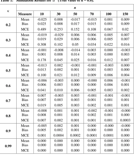
3.1 Biasness of estimators
as the mean of ˆ close to the true value of with the increase of sample size n or the concentration parameters of circular random errors.
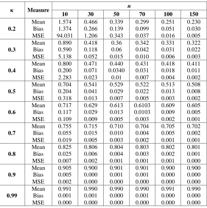
Also, we note from Table 1 and Table 2 that there is an inverse relationship between the
sample size n and the values of the
1
1 ˆ
(1 cos( ))
s
i i
MCE
s =
=
− − and2 1 1 ˆ ( ) s j j MSE
s =
=
− of the estimators ˆ and ˆ, respectively, these findings indicate the consistency of the estimators.Table 1: Simulation Results for ˆ (True value of α = 0.0).
3.2 Coverage probability of confidence intervals
The coverage probability of a confidence interval is the proportion of the time that the interval contains the true value of interest, see (Dodge; 2003). In this simulation study we construct intervals at 0.95 confidence level. Hence, the good indicator must give the coverage probability close to 0.95. The estimation of the parameters were repeated for different sample sizes (n = 30, 50, 100, and 150) and concentration parameter = 0.2, 0.4, 0.6, 0.8 and 0.99. The results of the simulations are given in Table 3 based on 1000 repetition times.
Results in Table 3 show that the observed coverage appears to be approximately equivalent to the confidence level, which reveals an excellent coverage of the confidence intervals.
Table 2: Simulation Results for ˆ
Table 3: Results for coverage percentage of confidence interval for and
n
κ 30 50 70 100 150
κ α
κ α
κ α
κ α
κ α
93.1 94.8
93.6 95.1
99.6 94.2
99.7 93.3
98.9 95.5
0.2
94.5 95.1
94.0 93.6
92.1 96.4
92.5 95.6
99.6 93.0
0.4
94.7 94.8
94.8 94.1
93.5 95.0
92.3 95.2
95.2 93.9
0.6
94.5 95.3
94.5 95.0
90.7 95.8
95.4 95.5
95.5 94.7
0.8
96.5 95.0
96.5 95.1
97.8 94.7
95.9 95.2
96.6 95.9
0.99
3.3 Robustness of the estimates
Robustness of an estimator is a useful property which gives a fair assurance that the existence of any possible outlier or violation of model assumptions will not have much effect on the parameters estimates. To assess the robustness, based on simulation study, where 5% of the generated data are contaminated start from observation d as follows:
*
[ ] [ ] (mod 2 ),
y d = y d +
where y d*[ ] and y d[ ] are the contaminated and original values of the dependent variable Yrespectively, and is the contamination level, where 0 1.
The results of simulation study show that, for data with highly concentrated error 0.6, the bias of ˆ is less than 0.3 for small samples (n=10) and less than 0.15 for moderate and large samples (n30). Regardless the concentration of error and the sample size, the optimum values of bias of are obtained for moderate levels of contamination 0.6 . It may be referred to the nature of the circular data, where the shift of 5% of the generated data by more than / 2 of its original values may lead to get closer to the majority of the data. Almost similar conclusion can be drawn for the concentration parameter.
4. Real Data Analysis
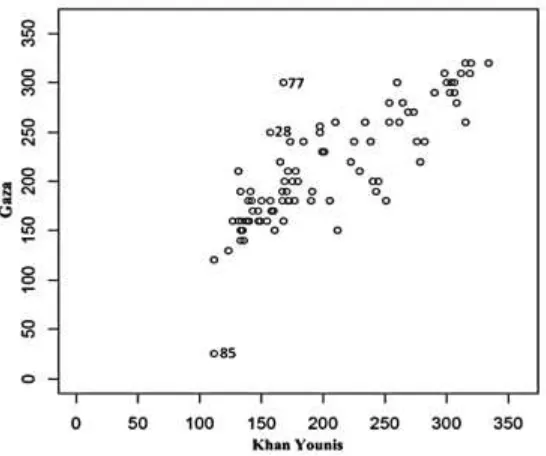
As an illustration of the proposed model, this section considers the measurements of wind directions that have been collected from two meteorological stations in two main cities in the Gaza Strip, namely Gaza and Khan Younis in Palestine. The data were provided by the Palestinian Metrological Authority, in 2007. It represent the monthly average wind directions every three hours a day viz, 0:00 mid night, 3:00 am, 6:00 am, 9:00 am, 12:00 noon, 15:00 pm, 18:00 pm and 21:00 pm. (Badawi 2013) analyzed the Palestinian wind data in order to establish a wind farm to reach the optimum electricity energy. Recently, (Abuzaid and Allahham 2015) modelled the data by using the simple circular regression model assuming the wrapped Cauchy error. The linear circular regression model between dependent and independent variables is given by
0.747 0.842 (mod 2 ),
Y = + X
4.1 Fitting the functional circular regression model with wrapped Cauchy error
Since the relationship between the wind directions of Gaza and Khan Younis is reasonably linear as shown in Figure 1; the simple functional circular regression model (1) is suggested to fit the data. The parameters estimates are obtained by applying the iterative procedure and after converting the data into radians. The initial values of 1 and
2
are taking to be 0.3.
Table 4 presents the estimates of parameters, their standard error and the 95% confidence intervals, where the convergence is occurred after 16 iterations. Hence, the estimate relationship for wind directions of Gaza and Khan Younis data set is given by
0.237 (mod 2 ),
Y = +X
where variable Y is the wind directions data for Gaza and the wind directions data for Khan Younis is the variable X .
Figure 1: Scatter plot of wind directions in Gaza versus KhanYounis
Table 4: Parameter estimation of circular functional model with wrapped Cauchy Errors
Parameter Estimate Standard Error Confidence Interval
ˆ
0.237 0.0024 (0.140, 0.333)
ˆ
0.843 0.0018 (0.759, 0.927)
(Abuzaid 2010) suggested a statistic to test the goodness-of-fit of circular models, A*( )
to be analogues the coefficient of determination in the linear regression models as given below:
* 1 2 ˆ
( ) cos ( i i),
A y y
n
where 0A*( ) 1. Therefore, the closer A*( ) to 1 indicates a better fitting the model. Thus, the goodness-of-fit for the model is A*( ) =0.799.
The obtained residuals were tested to follow the wrapped Cauchy distribution via Kolomogrov-Simrnov test, where the values of test for the errors of and are 0.0401 and 0.0321 with P-values 0.835 and 0.895, respectively.
5. Conclusions
A new linear functional relationship model for circular variables with a wrapped Cauchy errors has been proposed due to the attractive properties of wrapped Cauchy distribution. The maximum likelihood estimates of parameter has been obtained assuming equality of concentration parameters of errors. Estimation has been obtained iteratively since the closed-form expression for estimates are not available, by choosing a suitable initial values, the standard error of estimates as well as their confidence intervals are obtained by bootstrapping methods. Moreover, the proposed angular regression model has been applied on a real data set of wind directions at two cities in the Gaza strip.
References
1. Abuzaid, A. H. (2010). Some Problems for Outliers Circular Data. PhD Thesis, University of Malaya, Kuala Lumpur.
2. Abuzaid, A. and Allahham, N. (2015). Simple circular model assuming wrapped Cauchy error. Pakistan Journal of Statistics, 31 (4), 385-398.
3. Adcock, R. J. (1877). Note on the method of least squares, Analyst, 4, 183-184.
4. Adcock, R. J. (1878). A problem in least squares, Analyst, 5, 53-54.
5. Badawi, A. S. (2013). An Analytical Study for Establishment of Wind Farms in Palestine to Reach the Optimum Electrical Energy. Master thesis. The Islamic University of Gaza, Palestine.
6. Caires, S. and Wyatt, L. R. (2003). A linear functional relationship model for circular data with an application to the assessment of ocean wave measurements, J. Agric. Biol. Environ. Stat., 8 (2), 153-169.
7. Chernick, M. R. (1999). Bootstrap Method: A practitioner‘s Guide. Canada: John Wiley & Sons.
8. Dodge, Y. (2003). The Oxford Dictionary of Statistical Terms, OUP.
9. Downs, T. D. and Mardia, K. V. (2002). Circular regression. Biometrika, 89 (3), 683-697.
10. Hussin, A. G. (1997). Psuedo-replication in functional relationship with environmental application. Ph.D. Thesis. University of Sheffield, England.
12. Hussin, A. G. (2005). Approximating Fisher’s information for the replicated linear circular functional relationship model. Bull. Malays. Math. Sci. Soc., 28,(2), 1-9
13. Hussin, A. G., Abuzaid, A. H., Zulkifli, F. and Mohamed, I. B. (2010). Asymptotic covariance and detection of influential observations in a linear relationship model for circular data with application to the measurements of wind directions. ScienceAsia, 36, 249-253.
14. Hussin, A. G., Fieller, N. R. J. and Stillman, E. C. (2004). Linear regression for circular variables with application to directional data. Journal of Applied Science & Technology, 9, (1 & 2), 1-6.
15. Kendall, M. G. (1951). Regression, structural and functional relationship I, Biometrika, 38, 11-25.
16. Kendall, M. G. (1952). Regression, structural and functional relationship II, Biometrika, 39, 96-108.