The evaluation of binary classification tasks in economical prediction

(1)

369

Volume LVIII 36 Number 6, 2010

THE EVALUATION OF BINARY CLASSIFICATION

TASKS IN ECONOMICAL PREDICTION

M. Pokorný

Received: September 6, 2010

Abstract

POKORNÝ, M.: The evaluation of binary classiﬁ cation tasks in economical prediction. Acta univ. agric. et silvic. Mendel. Brun., 2010, LVIII, No. 6, pp. 369–378

In the area of economical classifi cation tasks, the accuracy maximization is o en used to evaluate classifi er performance. Accuracy maximization (or error rate minimization) suff ers from the assump-tion of equal false positive and false negative error costs. Furthermore, accuracy is not able to express true classifi er performance under skewed class distribution. Due to these limitations, the use of accu-racy on real tasks is questionable. In a real binary classifi cation task, the diff erence between the costs of false positive and false negative error is usually critical. To overcome this issue, the Receiver Ope-rating Characteristic (ROC) method in relation to decision-analytic principles can be used. One es-sential advantage of this method is the possibility of classifi er performance visualization by means of a ROC graph. This paper presents concrete examples of binary classifi cation, where the inade-quacy of accuracy as the evaluation metric is shown, and on the same examples the ROC method is applied. From the set of possible classifi cation models, the probabilistic classifi er with continuous output is under consideration. Mainly two questions are solved. Firstly, the selection of the best classi-fi er from a set of possible classiclassi-fi ers. For example, accuracy metric rates two classiclassi-fi ers almost equiva-lently (87.7 % and 89.3 %), whereas decision analysis (via costs minimization) or ROC analysis reveal diff ere nt performance according to target conditions of unequal error costs of false positives and false negatives. Secondly, the setting of an optimal decision threshold at classifi er’s output. For example, accuracy maximization fi nds the optimal threshold at classifi er’s output in value of 0.597, but the op-timal threshold respecting higher costs of false negatives is discovered by costs minimization or ROC analysis in a value substantially lower (0.477).

binary classiﬁ cation, bankruptcy prediction, classiﬁ er performance evaluation, accuracy maximiza-tion, receiver operating characteristic (ROC)

In the area of economical research, much atten-tion has been paid to development and improve-ment of many prediction methods and models so far. One of the typical tasks being solved is the bank-ruptcy and fi nancial distress prediction and related binary classifi cation task. Surprisingly, not so many studies pay attention to a more sophisticated clas-sifi er performance evaluation. Despite the fact the evaluation methodology critically aff ects the opti-mal classifi er selection and its use, not so suffi cient accuracy maximization (or error rate minimization) has been o en used. Other non-fi nancial literature criticizes accuracy maximization procedure as well. Detailed fi ndings can be found in Pokorny (2009)

within the present state analysis of this problem, where other authors are quoted.

In the area of medical research, the Receiver Ope-rating Characteristic (ROC) method has been widely used, which has the potential to solve the lack of a sophisticated evaluation methodology, includ-ing consideration of diff erent type I/II error costs. Moreover, it has the ability to visualize classifi er’s performance. Although the ROC is not completely unknown to the fi nancial research, its application is rare.

(2)

classi-ﬁ cation task, and to show the use of ROC analysis as an alternative evaluation method. This paper is based on results of F. Provost’s and T. Fawcett’s re-search and tries to popularize this topic. Results of this study can be used as a guide for the economical research mentioned above.

MATERIAL AND METHODS

Binary classiﬁ cation

The binary classifi cation task is confi ned to two class separation. The classifi er’s outcome can be treated as positive (P) or negative (N), and according to the true status of an instance being classifi ed, the clas-sifi cation result can be true positive (TP), true nega-tive (TN), false posinega-tive (FP, Type I Error) or false negative (FN, Type II Error). In case of bankruptcy prediction, a company could be rated as healthy (negative) or failing (positive). Many classifi cation models applicable on this task exist, solid theoreti-cal background can be found e.g. in Bishop (2006). This study focuses primarily on a so called proba-bilistic classifi er with continuous output. The clas-sifi er’s output is in the form of a probability or score – numeric value that represents the degree to which an instance is a member of a class. (Fawcett, 2004) The same author then follows: “These values can be strict probabilities, in which case they adhere to standard theorems of probability; or they can be general, uncalibrated scores, in which case the only property that holds is that a higher score indicates a higher probability.”.

Having a test set1_{of negative and positive samples}

(with true status of class membership), and a set of potential classiﬁ ers, the goal is to choose the best classiﬁ er according to target conditions of

applica-tion. Each of the classifi ers is populated with the test set, and at its output produces the outcome usua-lly in the form of a Gaussian distribution for either of the classes. Varying the decision threshold at the classifi er output to a suitable position, the fi nal form of the classifi er is obtained – a discrete

classi-fi er (Fawcett, 2004), and so the second goal is to set the optimal decision threshold. Samples rated above this threshold are classifi ed as positive, samples be-low are classifi ed as negative. One example of a typi-cal classifi er of this type is the neural network having sigmoidal activation function on its output neuron. The fi xed threshold of 0.5 would be an misleading approach because of relative score separation objec-tive, as describes Fawcett’s example (2004, p. 8).

The accuracy as an evaluation metric

Accuracy (error rate) is given by the ratio of correctly (incorrectly) classifi ed instances to all instances in the test set, i.e. (TP + TN)/(P + N). This type of met-ric is criticized by authors for its inability to diff er-entiate between type I and II error costs (both are assumed to be equal), but they do diff er in most practical tasks. Furthermore, accuracy doesn’t re-fl ect true classifi er’s performance under skewed class distribution. In reality, classifi ers o en face to a grater number of negative instances compared to positive instances. (Obuchowski, 2003; Faw-cett, 2004; Provost and FawFaw-cett, 2001, 1997; Provost, Fawcett and Kohavi, 1998) Accuracy evaluates classi-fi er’s performance with one number for both of the classes and for one setting of target conditions.

Another shortcoming of the accuracy metric is the indistinguishable performance evaluation of two diff erent scenarios, as depicted on Fig. 1 – example similar to Erkel and Pattynama (1998). The accuracy is the same for both of the situations, but for exam-ple, classifying almost all positives in the fi rst one encompasses wrong classifi cation of almost all nega-tives. On the other hand, classifying almost all posi-tives within the second scenario encompasses ap-proximately only half of false positives.

ROC analysis

ROC analysis is a method frequently used in medical research. Essential ROC metrics are the sensitivi ty and speciﬁ city. Sensitivity (or true positive rate, TPR) is the proportion of correctly classiﬁ ed positives (TP) among all positives (P), i.e. TPR = TP/P.

1 Not only one single test set should be used, for the purpose of variance measurement, several test sets should be used. (Fawcett, 2004). The same author then presents the so called ROC curves averaging.

(3)

Specifi city (or true negative rate, TNR) is the pro-portion of correctly classifi ed negatives (TN) among all negatives (N), i.e. TNR = TN/N. The opposite of specifi city is the false positive rate (FPR = FP/N), where FP is the number of negatives incorrectly classifi ed as positive. Similarly, false nega tive rate FNR = FN/P, where FN is the number of positives in-correctly classifi ed as negative.

Varying the decision threshold at classifi er’s con-tinuous output, the number of TP, FN, TN and FP changes, so does the sensitivity and specifi city, but both in opposite direction. Higher sensitivity results in lower specifi city and vice versa. Diff erent thresh-olds constitute set of points [FPR, TPR] resulting in a ROC Curve and so called ROC graph. ROC curve generation algorithm can be found for example in Fawcett (2004). The X-axis in a ROC graph repre-sents false positive rate, the Y-axis reprerepre-sents sensi-tivity. Discrete classifi er (i.e. with the output of P or N only) is represented by one point in the graph. The more north-west the point lies, the better solution has been found. Ideal point is [0, 1], which means zero false positive rate and 100% sensitivity. The dia-gonal line represents the so called line of chance, in other words, no information is carried by the classi-fi er, and real classiclassi-fi er should always be above this line. Classifi ers laying under the line can easily be reversed to the upper le space by reverting their decisions. (Fawcett, 2004; Obuchowski, 2003; Pro-vost and Fawcett, 2001, 1997; ProPro-vost, Fawcett and Kohavi, 1998; Erkel and Pattynama, 1998)

“ROC graphs illustrate the behavior of a clas-sifi er without regard to class distribution or er-ror costs, and so they decouple classifi cation performance from these factors”. (Provost and Faw-cett, 2001, 1997) Similarly, Obuchowski (2003) men-tions ROC key characteristics. By treating both of the errors (FP, FN) separately, this method makes it possible to prioritize one type of error over another. Moreover, the ability to visualize the classifi er’s per-formance facilitates inherent analysis.

For the purpose of classifi er performance com-parison, it is usually easier to compare a single num-ber then two values of sensitivity and specifi city. The Area Under the ROC Curve (AUC) is an example of such metric and measures classifi er discrimina-tive power across all possible thresholds (or target conditions). Thereby AUC eliminates the infl uence of the decision threshold value on sensitivity and speci fi city. (Erkel and Pattynama, 1998). Perfect clas-sifi er has the AUC 1.0 (100 %), the area under the line of chance equals to 0.5 (50 %). For other interpreta-tions of the AUC, see Obuchowski (2003, p. 5).

One major drawback associated with the classi-ﬁ er comparison based on the AUC is that usually only part of the curve is practically relevant. (Obu-chowski, 2003; Erkel and Pattynama, 1998) For exa-mple, if we assume target conditions of high FN costs and relatively high occurrence of positive in-stances, the upper right part of the ROC graph is relevant. The target conditions can be visualized as a line in a ROC graph – according to Provost and

Fawcett (2001, 1997), this line is called iso-perfor-mance line with a slope s given by the formula below, and all classiﬁ ers corresponding to points on the line have the same expected costs. Using the exa-mple above, the iso-performance line would have a small slope and as a tangent to a ROC curve would be located in the upper right part.

TP₂−TP₁ p(n)C(FP) s =     FP2−FP1 p(p)C(FN)

where p(p) is the prior probability of a positive exam-ple, p(n) = 1 −p(p) is the prior probability of a nega-tive example, C(FP) and C(FN) are the costs of false positive and false negative errors.

Obuchowski (2003) states that “whenever the ROC curves of two tests cross (regardless of whether or not their areas are equal), it means that the test with superior accuracy (ie, higher sensitivity) de-pends on the FPR range; a global measure of ac-curacy, such as the ROC curve area, is not helpful here.” Only if one model dominates in the whole ROC space (all other curves are below the curve of this test), this model can be said as the best one. (Pro-vost and Fawcett, 2001, 1997; Pro(Pro-vost, Fawcett, Ko-havi, 1998) Obuchowski (2003) then suggests seve-ral alternatives for the situation of crossing ROC curves: use of the ROC curve to estimate sensitivity at a fi xed false positive rate (or false positive rate at a fi xed sensitivity), or use of the partial area under the ROC curve (the area between two false positive rates, or the area between two false negative rates). Similar recommendations can be found in Erkel and Pattynama (1998). Obuchowski (2003, p. 7, Fig. 4) or Erkel and Pattynama (1998, p. 92, Fig. 4) depict this situation, similarly Fig. 2 below shows two ROC curves corresponding to two classifi ers from Fig. 1 of this paper. Obviously, the second classifi er would be more appropriate in case of high FN costs and

(4)

high prevalence of positives, its ROC curve lies more north-west in the relevant part of the ROC graph.

To sum up, the ROC curve represents classiﬁ er’s behavior in every possible situation, the iso-perfor-mance line represents speciﬁ c target conditions, by combining them, the optimal decision threshold can be found.

By the way, Provost and Fawcett invented a com-plex method called ROC Convex Hull, which em-ploys principles of the ROC analysis, decision analy-sis and computation geometry, and which is able to identify set of methods that are potentially optimal under any cost and class distribution. (See Provost and Fawcett, 2001, 1997; Fawcett, 2004 for details.)

Data

To demonstrate the use of ROC analysis for the cost-sensitive classiﬁ er evaluation, six data sets were generated. Each data set represents classiﬁ er’s out-put score (as explained in the Material and Meth-ods chapter) in a form of Gaussian distribution from interval 0-1 separately for negative and posi-tive instances on a test set. Such output can be ob-tained for example from a neural network having the sigmoidal activation function at the output unit.

Test 1 data set (i.e. the output score of classiﬁ er 1 for a given test set of samples) contains 100 nega-tive and 100 posinega-tive instances (mean ± std.

devia-tion negatives/positives: 0.2 ± 0.1/0.8 ± 0.1) and rep-resents an ideal classifi er with no overlap between both of the classes. Test 2 data set consists of 200 in-stances for each class (mean ± std. deviation nega-tives/positives: 0.35 ± 0.1/0.65 ± 0.1), having slight overlap. More realistic are the test 3 (mean ± std. de-viation negatives/positives: 0.4 ± 0.12/0.6 ± 0.12) and test 4 (mean ± std. deviation negatives/posi-tives: 0.45 ± 0.12/0.55 ± 0.12) data sets, where nega-tive samples (3200) outnumber posinega-tive samples (800). Test 4 has considerable overlap compared to test 3. Last two tests, test 5 (mean ± std. devia-tion negatives/positives: 0.5 ± 0.15/0.75 ± 0.07) and test 6 (mean ± std. deviation negatives/positives: 0.25 ± 0.07/0.5 ± 0.15) with balanced classes of 1000 samples per class demonstrate the eff ect of reversed distribution of positive and negative samples on bi-nary classifi cation.

Statistical characteristics are shown in Tab. I–III, histograms (number of positive and negative sam-ples from the test set being classiﬁ ed with the classi-ﬁ er’s output score in one of 20 groups from interval 0–1) are depicted in Fig. 3–5.

RESULTS AND DISCUSSION

Two questions have to be solved before applying a new classiﬁ er. Firstly, all available classiﬁ ers have

I: Classiﬁ er 1 and 2 statistical characteristics of the class output score

Classiﬁ er 1 Classiﬁ er 2

Negatives n = 100 Positives n = 100 Negatives n = 200 Positives n = 200

Mean 0.192 0.802 0.351 0.647

Std. deviation 0.096 0.092 0.107 0.1

Median 0.189 0.8 0.36 0.652

Min 0.005 0.517 0.057 0.379

Max 0.431 0.970 0.656 0.978

II: Classiﬁ er 3 and 4 statistical characteristics of the class output score

Negatives n = 3 200 Positives n = 800 Negatives n = 3 200 Positives n = 800

Mean 0.399 0.594 0.449 0.55

Std. deviation 0.119 0.119 0.12 0.121

Median 0.401 0.594 0.448 0.55

Min 0.009 0.224 0.019 0.191

Max 0.773 0.943 0.874 0.895

III: Classiﬁ er 5 and 6 statistical characteristics of the class output score

Negatives n = 1 000 Positives n = 1 000 Negatives n = 1 000 Positives n = 1 000

Mean 0.508 0.752 0.253 0.509

Std. deviation 0.153 0.069 0.07 0.149

Median 0.511 0.752 0.253 0.508

Min 0.098 0.506 0.044 0.09

(5)

to be compared according to their classifi cation per-formance and the best one has to be chosen. Se-condly, an optimal decision threshold (cut-off ) must be set. Both tasks depend on target conditions, i.e. target error costs of FP and FN and target distribu-tion of negatives and positives. Choosing the right metric for classifi er performance evaluation is criti-cal for both of the tasks.

Classiﬁ er 1 shows a classiﬁ er which is able to dis-tinguish negatives from positives samples without any errors. In this situation, the setting of a decision

threshold is straightforward and lies in the lowest positive instance 0.51735, or due to the classifi er generalization, it could be more convenient to set the decision threshold to the middle of the interval between the highest negative and lowest positive in-stance. Any value lying above this threshold is clas-sifi ed as a positive instance, any value lying below this threshold is classifi ed as a negative instance. No errors (FP, FN) are produced with this threshold. In this case, the accuracy (error minimization) is able to express true classifi er performance and set the op-3: Histogram of the output score of classifier 1 (neg./pos.: 100/100; mean ± std. dev. 0.2 ± 0.1/0.8 ± 0.1), and classifier 2 (neg./pos.: 200/200; mean ± std. dev. 0.35 ± 0.1/0.65 ± 0.1)

4: Histogram of the output score of classifier 3 (neg./pos.: 3200/800; mean ± std. dev. 0.4 ± 0.12/0.6 ± 0.12), and classifier 4 neg./ pos.: 3200/800; mean ± std. dev. 0.45 ± 0.12/0.55 ± 0.12)

(6)

timal threshold, even if the target misclassiﬁ cation costs C(FP) and C(FN) were not the same.

Accuracy used for setting a decision threshold Inappropriate use of accuracy for the purpose of setting an optimal decision threshold shows classi-fi er 2. Accuracy maximization (or error rate minimi-zation) sets the threshold in the intersection of the negative and positive class. In case of classifi er 2, maximal accuracy of 93.25 % (minimal error rate of 6.75 %) is reached by setting the threshold to the value of 0.51464 or 0.48917. If we assume a situa-tion of target costs e.g. C(FP) = 1 and C(FN) = 5, to-tal misclassifi cation costs would be 91 (for the fi rst threshold) or 79 (for the second threshold). On the contrary, the costs minimization method sets the threshold to a lower value 0.47019, which produces lower total costs of 57. This clearly shows, that accu-racy maximization (error rate minimization) doesn’t set the optimal threshold in case of unequal error costs. The threshold set by this metric would be op-timal in case of equal error costs.

Similar results can be shown on classifi ers 3 and 4. The threshold set by accuracy maximization is too high compared to the threshold set be costs minimi-zation. Costs minimization refl ects higher costs of FN, thereby prefers correct classifi cation of positives (higher true positive rate, TPR) at the expense of in-correct classifi cation of many negatives (higher false positive rate, FPR). Tab. IV describes this phenome-non for classifi ers 1–4.

One question may arise – why are there two opti-mal thresholds according to the accuracy maximiza-tion? Let’s demonstrate this phenomenon on classi-fi er 4 (similar eff ect can be found with classiclassi-fi ers 2, 3 and 6):

Instead of considering two optimal thresholds, it might be more correct to consider the average value of score lying between both of the minimums.

Accuracy used for classiﬁ er performance comparison

Inappropriate use of accuracy for the purpose of classifi er performance comparison is demonstrated on two examplwes. Firstly, consider an example of two classifi ers A and B whose output score distri-butions together with target conditions are shown on Fig. 6. Let’s assume that this case is characteristic with high disproportion between FP and FN costs, e.g. C(FP) = 1 and C(FN) = 150, and the distribution is balanced N/P = 100/100 for simplicity. According to accuracy maximization, classifi er A should be better than its counterpart because of its lower error rate. But then, if diff erent error costs are taken into con-sideration, classifi er B is obviously better than clas-sifi er A – see costs equal to FP in both situations. The reason why accuracy maximization doesn’t work well in this case is that accuracy tacitly assumes equal error costs, i.e. C(FP) = C(FN).

Similar behavior can be shown on classifi ers 5 and 6. For the purpose of classifi er comparison and se-lection, the accuracy is not usable here. According to the accuracy maximization, classifi er 5 has accu-racy of 87.7 % (in threshold 0.63527), classifi er 6 has accuracy of 89.3 % (in threshold 0.37448 or 0.37381), and so both classifi ers are rated almost equivalently. But if diff erent error costs are taken into conside-ration, the situation is completely diff erent. Having C(FP) = 1 and C(FN) = 5, classifi er 5 has minimal costs of 339 (in threshold 0.6016), classifi er 6 has minimal costs 641 (in threshold 0.31339) and is much worse classifi er for this situation. Similarly, having C(FP) = 5 and C(FN) = 1, classifi er 5 has mini-IV: Accuracy maximization vs. costs minimization, classifi ers 1–4

Classiﬁ er

Accuracy maximization

(Error rate minimization) Costs minimization Accuracy

(Error rate) threshold (s)Related [FPR, TPR]Related Related costs* Total costs* thresholdRelated [FPR, TPR]Related

Classiﬁ er 1 ₍₀₎1 0.51735 [0, 1] 0 0 0.51735 [0, 1]

Classiﬁ er 2 _(0.0675)0.9325 0.51464; _0.48917 [0.055, 0.920];_{[0.070, 0.935]} 91;₇₉ 57 0.47019 [0.110, 0.965]

Classiﬁ er 3 _(0.1435)0.8565 0.59754; _0.59679 [0.052, 0.489];_{[0.053, 0.493]} 2210;₂₁₉₈ 1412 0.47702 [0.251, 0.848]

Classiﬁ er 4 _(0.19025)0.80975 0.67699; _0.67682 [0.026, 0.153];_{[0.026, 0.154]} 3473;₃₄₆₉ 2329 0.47976 [0.390, 0.730]

* C(FP) = 1, C(FN) = 5

Score # N/P Score FP FN Errors

203 P 0.67791 83 680 763

204 P 0.67734 83 679 762

205 P 0.67699 83 678 761  min 1 (761/4000 = 0.19025)

206 N 0.67698 84 678 762

207 P 0.67682 84 677 761  min 2 (the same error rate)

208 N 0.67593 85 677 762

(7)

6: Inadequate use of accuracy for classifier performance comparison

V: Accuracy maximization vs. costs minimization, classiﬁ ers 5–6

Accuracy maximization (Error rate minimization)

Classiﬁ er _{(Error rate)}Accuracy Related threshold (s) Related [FPR, TPR]

Classiﬁ er 5 _(0.1235)0.8765 0.63527 [0.212, 0.965]

Classiﬁ er 6 _(0.1075)0.8925 0.37448;_0.37381 [0.043, 0.828];_{[0.044, 0.829]}

Costs minimization – C(FP) = 1, C(FN) = 5

Classiﬁ er Total costs Related threshold Related [FPR, TPR]

Classiﬁ er 5 339 0.60160 [0.274, 0.987]

Classiﬁ er 6 641 0.31339 [0.201, 0.912]

Costs minimization – C (FP) = 5, C(FN) = 1

Classiﬁ er Total costs Related threshold Related [FPR, TPR]

Classiﬁ er 5 720 0.72030 [0.081, 0.685]

Classiﬁ er 6 305 0.40996 [0.011, 0.750]

(8)

mal costs of 720 (in threshold 0.7203), classiﬁ er 6 has minimal costs of 305 (in threshold 0.40996) and is much better classiﬁ er for this situation. Tab. V con-tains further details (FPR, TPR).

ROC analysis in general

In addition to the methods discussed so far (accu-racy maximization, costs minimization), the ROC analysis delivers visualization of classiﬁ er perfor-mance through a so called ROC graph. The ROC graph consists of a ROC curve that shows classiﬁ er performance in a form of [FPR, TPR] pairs across all possible decision thresholds.

On Fig. 7a, there are ROC curves of classifi er 1 and classifi er2. Classifi er 1 curve is composed by three points [0, 0] – [0, 1] – [1, 1], and represents an ideal classifi er with the area under the ROC curve (AUC) equal to 1 (100 %). Classifi er 2 has lower curve with AUC 0.97837 (97.8 %). ROC graph for classifi er 3 and 4 is shown on Fig. 7b. Classifi er 3 curve is above classifi er 4 curve in the whole ROC space, so we can conclude, that classifi er 3 would be a better choice than classifi er 4 in all possible decision thresholds and target conditions. Superiority of classifi er 3 over classifi er 4 can be expressed also with the AUC, clas-sifi er 3 has AUC of 87.5 %, clasclas-sifi er 4 AUC is 72.4 %.

ROC analysis and setting an optimal decision threshold

ROC analysis itself is not able to set an optimal decision threshold. But if it is combined with the iso-performance line, same results can be achieved as with the costs minimization, but with the luxury of visualization. The procedure is demonstrated on classiﬁ er 3 (Fig. 7b).

ROC curve of classiﬁ er 3 shows its behavior across all possible thresholds. Iso-performance line a, or its slope respectively, is given by target conditions, i.e. probability of a negative instance p(N) = 4/5 (3200/4000), probability of a positive in-stance p(P) = 1/5 (800/4000), and costs C(FP) = 1, C(FN) = 5. According to the formula in the theoret-ical section, the resulting slope equals to 4/5. The tangent of the iso-performance line a to the ROC curve of classiﬁ er 3 gives us the optimal decision threshold (emphasized with a circle). This point cor-responds to the costs minimization result, i.e. the threshold 0.47702 with [FPR, TPR] = [0.251, 0.848] (see Tab. IV).

Besides the target situation of unequal error costs, also the situation of equal misclassiﬁ cation costs C(FP) = C(FN) is shown through the line b. Line slope is 4/1, the resulting point is at [FPR, TPR] cor-responding to the threshold set by error minimiza-tion (see Tab. IV).

Again, costs minimization itself seems to be suf-ﬁ cient method for this problem, but what if the tar-get conditions (e.g. misclassiﬁ cation costs) are not known, or are known only approximately? In this case, described visualization of the ROC curve and iso-performance line could be highly valuable.

ROC analysis and classiﬁ er performance comparison

In a ROC graph, the classiﬁ er performance can be compared visually, which is the ﬁ rst and quickest way. The more north-west the ROC curve is, the bet-ter (see Fig. 7 and 8).

The performance can be compared numerically according to the AUC. Higher AUC value means

(9)

ter performance. Tab. VI shows AUC of all classiﬁ ers discussed so far.

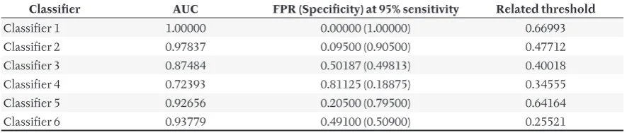
However, one considerable drawback about AUC must be emphasized – this metric is usually irrele-vant when ROC curves cross. This is the case of clas-sifi er 5 and clasclas-sifi er 6 (see Fig. 8). The AUC rates both of the classifi ers almost equivalently (92.7 % and 93.8 % for classifi er 5 and classifi er 6 respec-tively) because this type of metric measures the discriminative power across all possible thre sho-lds, i.e. without regard to target conditions. But as was already shown, both classifi ers are completely diff erent, either successful in diff erent target condi-tions (classifi er 5 in a situation of higher C(FN), clas-sifi er 6 in a situation of higher C(FP)).

In this case, several other metrics are suggested. One of them could be the comparison according to the FPR (or specifi city) at a fi xed sensitivity level. This metric is useful in a situation of higher C(FN). Tab. VI compares all classifi ers of this study not only with the AUC metric, but also with the FPR (specifi city) at fi xed sensitivity of 95 % (other valu es of sensitivity can be used as well, e.g. 92 %, 90 %). Here is obvious, that classifi er 5 outperforms clas-sifi er 6 – specifi city at fi xed 95% sensitivity of classi-fi er 5 (79.5 %) is higher than speciclassi-fi city of classiclassi-fi er 6 (50.9 %).

The same eff ect can be shown in a ROC graph. On Fig. 8, only the right-upper part of the ROC graph is practically relevant, and here the ROC curve of clas-sifi er 5 lies above the curve of clasclas-sifi er 6. Similarly, the case of higher C(FP) shi s the area of interest to the le -lower part of the ROC graph, where classi-fi er 6 outperforms classiclassi-fi er 5.

Optimal decision threshold is set by the iso-per-formance line c touching the ROC curve of classi-ﬁ er 5, or line d touching the ROC curve of classiﬁ er 6 for either of the target conditions. Line c represents target conditions p(P) = p(N) = 1/2, C(FP) = 1, C(FN) = 5, so the line slope equals to 1/5, and resulting point on the ROC curve corresponds to the threshold 0.60160 with [FPR, TPR] = [0.274, 0.987] calculated by costs minimization. Line d represents target con-ditions p(P) = p(N) = 1/2, C(FP) = 5, C(FN) = 1, so the line slope equals to 5/1, and resulting point on the ROC curve corresponds to the threshold 0.40966 with [FPR, TPR] = [0.011, 0.750] calculated by costs minimization.

So ware, platform and algorithms used

Receiver Operating Characteristic:

Own implementation based on Fawcett (2004, p. 13 – algorithm 2, p. 16 – algorithm 3), imple-mented in Borland Delphi 7 Professional.

Accuracy maximization/Error rate minimization, Costs minimization:

Own implementation based on ROC points – fi nd minimum of errors (costs) produced by every pos-sible classifi er’s threshold (classifi er’s output score), equally scored instances are treated as one instance (threshold considering errors/costs for all equally scored instances). Modifi ed so ware application for ROC above.

Platform:

MS Windows XP Professional, Linux Mandriva 2009.1

VI: Classiﬁ er performance numerical comparison

Classiﬁ er AUC FPR (Speciﬁ city) at 95% sensitivity Related threshold

Classiﬁ er 1 1.00000 0.00000 (1.00000) 0.66993

Classiﬁ er 2 0.97837 0.09500 (0.90500) 0.47712

Classiﬁ er 3 0.87484 0.50187 (0.49813) 0.40018

Classiﬁ er 4 0.72393 0.81125 (0.18875) 0.34555

Classiﬁ er 5 0.92656 0.20500 (0.79500) 0.64164

Classiﬁ er 6 0.93779 0.49100 (0.50900) 0.25521

SUMMARY

(10)

(87.7 % and 89.3 %), whereas decision analysis (via costs minimization) or ROC analysis reveal diff er-ent performance according to target conditions of unequal error costs of false positives and false nega-tives. Secondly, the setting of an optimal decision threshold at classifi er’s output. For example, accu-racy maximization fi nds the optimal threshold at classifi er’s output in value of 0.597, but the optimal threshold respecting higher costs of false negatives is discovered by costs minimization or ROC analy-sis in a value substantially lower (0.477).

SOUHRN

Evaluace binárních klasiﬁ kačních úloh v ekonomické predikci

V oblasti ekonomických klasifi kačních úloh je maximalizace přesnosti často používanou metrikou pro hodnocení klasifi kačního výkonu. Maximalizace přesnosti (resp. minimalizace chybovosti) trpí předpokladem rovných nákladů chyb typu falešná pozitivita a falešná negativita. Kromě toho není přesnost schopna vyjádřit pravý výkon klasifi kátoru v situaci nerovnoměrného rozložení tříd. Vzhledem k těmto omezením je použití přesnosti v reálných úlohách diskutabilní. V reálné binární klasifi -kační úloze je rozdíl mezi náklady falešné pozitivity a falešné negativity obvykle kritický. K překonání tohoto problému je použita metoda ROC ve spojení s principy rozhodovací analýzy. Jednou z pod-statných výhod této metody je možnost vizualizace klasifi kačního výkonu prostřednictvím ROC grafu. Tato studie prezentuje konkrétní příklady binární klasifi kace, kde je ukázána neadekvátnost přesnosti jako evaluační metriky, a na stejných příkladech je dále aplikována metoda ROC. Z mno-žiny dostupných klasifi kačních modelů je uvažován pravděpodobnostní klasifi kátor se spojitým vý-stupem. Zejména jsou řešeny dvě otázky. Za prvé výběr nejlepšího klasifi kátoru z množiny dostup-ných klasifi kátorů. Například metrika přesnosti hodnotí dva klasifi kátory téměř ekvivalentně (87,7 % a 89,3 %), zatímco rozhodovací analýza (prostřednictvím minimalizace nákladů) nebo ROC analýza odhalují rozdílný výkon podle cílových podmínek nerovných nákladů falešných pozitivit a falešných negativit. Za druhé nastavení optimální rozhodovací hraniční hodnoty na výstupu klasifi kátoru. Na-příklad maximalizace přesnosti nachází optimální hraniční hodnotu na výstupu klasifi kátoru v hod-notě 0,597, avšak optimální hraniční hodnota respektující vyšší náklady falešných negativit je nale-zena nákladovou minimalizací nebo ROC analýzou v hodnotě podstatně nižší (0,477).

binární klasiﬁ kace, predikce bankrotu, hodnocení výkonu klasiﬁ kátoru, maximalizace přesnosti, metoda ROC

REFERENCES

BISHOP, C. M., 2006: Pattern Recognition and Machine Learning. New York: Springer, 738 p. ISBN 0-387-31073-8.

ERKEL, A. R., PATTYNAMA, P. M. T., 1998: Receiver operating characteristic (ROC) analysis: Basis prin-ciples and applications in radiology. European Jour-nal of Radiology, 27: 88–94. ISSN 0720-048X. FAWCETT, T., 2004: ROC Graphs: Notes and Practical

Considerations for Researchers. HP Labs Tech Report HPL-2003-4. 2nd_{version. Kluwer Academic}

Pub-lishers. [online]. on the Internet: [quoted 2010-09-01]. Accessible.

<http://home.comcast.net/˜tom.fawcett/public html/papers/ROC101.pdf>.

OBUCHOWSKI, N. A., 2003: Receiver operating characteristic curves and their use in radiology. Ra-diology, 229: 3–8. ISSN 1527-1315.

POKORNÝ, M., 2009: The application of neural networks and ROC method in classiﬁcation tasks of economical

pre-diction. Dissertation theses. Brno, Mendel Univer-sity, Faculty of Business and Economics, Depart-ment of Informatics.

PROVOST, F., FAWCETT, T., 1997: Analysis and Vi-sualization of Classiﬁer Performance: Compari-son under Imprecise Class and Cost Distributions. In: HECKERMAN, D., PREGIBON, D., UTHUR-USAMI, R. (ed.) Proceedings of the Third International Conference on Knowledge Discovery and Data Mining. ISBN 978-1-57735-027-9.

PROVOST, F., FAWCETT, T., 2001: Robust Classiﬁcation for Imprecise Environments. Ma-chine Learning Journal, 42, 3: 203–231. ISSN 0885-6125.

PROVOST, F., FAWCETT, T., KOHAVI, R., 1998: The Case Against Accuracy Estimation for Compar-ing Induction Algorithms. In: SHAVLIK, W. J. (ed.) Proceedings of the Fi eenth International Conference on Machine Learning. Morgan Kaufmann Publishers. ISBN 1-55860-556-8.

Address