Formulation of the Equilibrium Equations
of Transversely Loaded Elements taking
Shear Deformation into Consideration
Onyeyili I. O.
Department of Civil Engineering Nnamdi Azikiwe University Awka
Anambra State
Okonkwo V. O.*
Department of Civil Engineering Nnamdi Azikiwe University Awka
Anambra State
[email protected], 08037755728 Abstract
In this work a mathematical model for the consideration of deformation due to shearing forces in structural analysis was formulated. The stiffness matrix for a prismatic element taking shear deformation into account was developed. The force/load vectors for various cases of transversely loaded elements taking shear deformation into consideration were also formulated and these were presented in tables synonymous to the tables of ‘end forces due to unit end displacements’ and ‘fixed end moments on transversely loaded elements’ found in many structural analysis textbooks. These tables will enable an easy implementation of the effects of deformation due to shear forces in structural analysis when using the stiffness method.
Keywords: Stiffness, shear deformation, degrees of freedom, prismatic members, modulus of elasticity in shear
Introduction
The analysis of indeterminate structures requires the writing of compatibility equations (equations for deformation) for selected points (nodes) in the structure (Nash, 1998; Gere, 2004). Known causes of deformation of the structure are the internal stresses: bending moment, shearing forces, axial forces and twisting moments (Ghali and Neville, 1996). Amongst these, deformation due to bending moment dominates (Hibbeler 2006) and the deformations due to other stresses are very often ignored. For short and deep beams shear deformation is considerable and its consideration is necessary (Narayanan, 2007). However most classical methods of analysing structural frames eg slope deflection, moment distribution and clapeyron’s theorem ignore the deformation due to shear hence the need for a model to facilitate its easy integration into the normal processes of structural analysis in our manual calculations.
Model
The analysis of structures by the stiffness method involves the writing of equilibrium equations for the degrees of freedom (coordinates) of the structure (Jenkins, 1990). The equilibrium equation for the analysis of an
element is given by . . . (1)
Where [k] is the element stiffness matrix, it is a 12 x 12 matrix for a space element (elements that can deform in all three coordinate axes) and a 6 x 6 for a plane element (elements that deform in only one plane). {q} is the vector of external forces applied at any of the nodes and which coincide with one of the degrees of freedom for which the equilibrium equations were written. {d} is the vector of displacements at the coordinates or degrees of freedom of the element.
When there is no external force on any of the degrees of freedom or coordinates equation (1) is rewritten as 0 . . . . . . (2)
where {qo} is the vector of reactive end forces on the transversely loaded element when displacements at its coordinates (degrees of freedom) are restrained.
End Forces on Transversely Loaded Elements
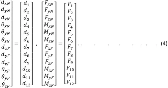
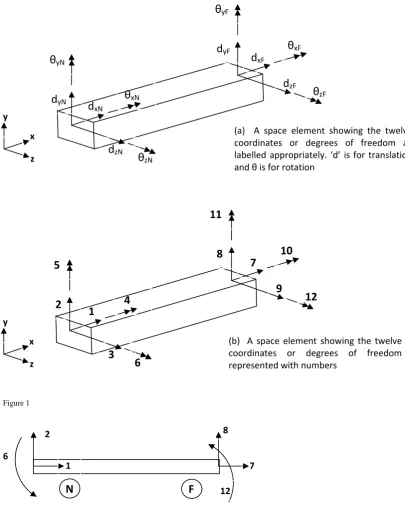
Here it will be illustrative to represent each coordinate (degree of freedom) with a number. This is shown in Figure 1(a) below. Figure 1(a) & (b) shows the 12 degrees of freedom of a space element and their representation with numbers. These numbers are used here for convenience. ‘1’ represents dxN ie the translation in the direction of the x axis at the near end ‘N’ and ‘2’ represents dyN ie the translation in the direction of the local y axis at the near end ‘N’. ‘11’ is θyF ie the rotation about the local y-axis at the far end and so on. Therefore
, . . . . . . . . . (4)
Numbers 1 – 6 is at the near end ‘N’ while 7 – 12 are at the Far end ‘F’.
MxN is the twisting moment at the near end ‘N’
MyN is the moment about the y axis at the near end
FyN is the axial force in the direction of the y axis acting at the near end
FxN is the axial force in the direction of the x axis acting at the near end etc
The sign convention for the translations is positive when it points in the direction shown in Figure 1 while the rotations are positive when anticlockwise.
For a space element
. . . . . . (5)
⋯ ⋯
⋮ ⋮ ⋮ ⋯⋱
⋯
Figure 4 For a plane element
If the plane element is lying in the xy plane (see Figure 2) and all the external loads on it act in the same plane then
0
If the deformation in these coordinates is zero then the forces (or moments for rotations) in these coordinates will also be zero.
0
. . . . . . . . (7)
. . . . (8)
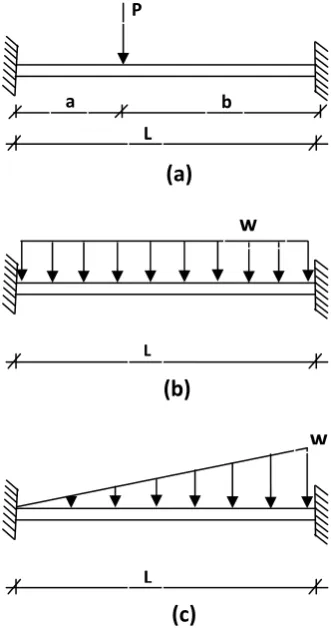
Consider the transversely loaded beam of Figure 3(a).
Reducing it to a basic system (A system that is statically determinate and geometrically stable)
X1 and X2 are the redundant forces and their directions of action are coordinates 1 and 2 respectively. The third redundant force (a horizontal force) was ignored because no axial force is expected.
From the principle of virtual work, deformations can be calculated (ignoring axial deformation) using
. . . . (9)
(Megson, 2005)
Where
κ is a shape factor which depends on the shape of the member’s cross-section.
Where , are the virtual internal stresses while M, V are the real/actual internal stresses. E is the modulus of elasticity of the structural material
A is the cross-sectional area of the element
G is the modulus of elasticity in shear, (Ugural and Fester,2003) where v is poisson’s ratio I is the moment of inertia of the section about the axis of bending.
Using equation (9), d11 (ie deformation in coordinate 1 due to a unit force in coordinate 1) can be evaluated by integration or graphically using a structural engineering table to obtain
3
3
In like manner other influence cooefficients are evaluated 6
6
3
3
The deformation at coordinate 1 due to the external load P is d10 while that in coordinate 2 is d20.
6 3 2
X1
X2
6 2 3
The compatibility or canonical equations for the structure (considering its two degrees of freedom 1 & 2) are given by
. . . . . (10)
X1 and X2 are evaluated from equation (10) to obtain
6 2
12
6 2
12
These are substituted into a superposition equation which is the sum of the forces in the basic system plus the contribution of the redundant forces. It is written as
. . . . . . . (11)
Where is the internal stress in the indeterminate system, is the values of the internal stresses when a unit value of the ith redundant acts on the basic system. is the internal stresses in the basic system due to the external loads. The values of X1 and X2 are substituted into equation (11) and solved to obtain
6 2
12
6 2
12
Consider the transversely loaded beam of Figure 3(b).
This is reduced to a basic system, a system that is statically determinate and geometrically stable (see figure 4). X1 and X2 are the redundant forces and their directions of action are coordinates 1 and 2 respectively. The flexibility matrix for this structure is the same as that for Figure 3(a). The deformation at coordinate 1 due to the external load w is d10 while that in coordinate 2 is d20 and are evaluated by integration or graphically using a structural engineering table to obtain
24
24
These are substituted into equation (10) to obtain
12
12 These are substituted into equation (11) to obtain
12
12
This shows that its end moments are not affected by shear deformation.
Consider the transversely loaded beam of Figure 3(c).
external load w is d10 while that in coordinate 2 is d20 and are evaluated by integration or graphically using a structural engineering table to obtain
7 360
45
These are substituted into equation (10) to obtain
45 15 12
20 10 12 X1 and X2 are substituted into equation (11) to obtain
45 15 12
20 10 12
The same processes were carried out on other transversely loaded beams to obtain their fixed end moments. From the equations of statics and by substituting the table of fixed end forces in beams of constant
flexural rigidity due to transverse loads was developed and presented below.
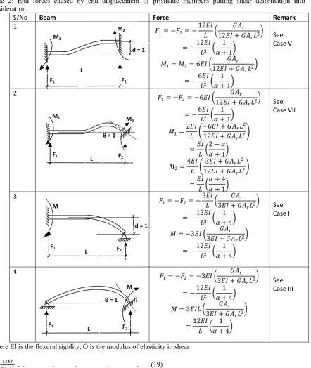
Table 1: End forces on transversely loaded prismatic members putting shear deformation into consideration.
S/No Beam Force
1
2
∝ 2
∝ 1
2
∝ 2
∝ 1
1
∝ 1
1
∝ 1
2
12
12
2
2
3
∝
∝
120
5 ∝ 6
∝ 1
6 1
1 10 ∝ 1
3 1
1 20 ∝ 1
M2
M1
F2
F1
P
L
a b
M2
M1
F1 L F2
w
L
w
F1 F2
M2
4
2 ∝
∝ 1
2 ∝
∝ 1
6 ∝ 1 6
∝ 1
5
2 2
∝ 4
1 2 2
∝ 4
1 2 2
∝ 4
6
2 1 ∝ 4
2 ∝ 5 ∝ 4
2 ∝ 3 ∝ 4
7
4 15
1 ∝ 4
3 1 2
4 5
1
∝ 4
3 1 4 5
1
∝ 4
8
2 3 2 ∝
4 ∝
2 3 2
4 ∝ 1
∝ 4
F1 L F2
a b
M M2
M1
M
F2
F1
w
L
F2
F1
M
L
w
MF2
F1 L
a b
P
M1
F2
F1 L
a b
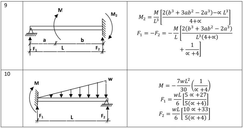
9
2 3 2 ∝
4 ∝
2 3 2
4 ∝ 1
∝ 4
10
7 30
1 ∝ 4
6
5 ∝ 27 5 ∝ 4
6
10 ∝ 33
5 ∝ 4
Note that in the table above clockwise moments were taken as positive while anticlockwise moments were negative. In the derivation of the end moments and forces, moments that keep the bottom fibres in tension were taken as positive while those that keep the top fibres in tension were negative. Likewise shearing forces that cause the system to move upwards were treated as positive in the table. In the derivation, shearing forces that cause the system to rotate clockwisely were positive while the opposite were negative.
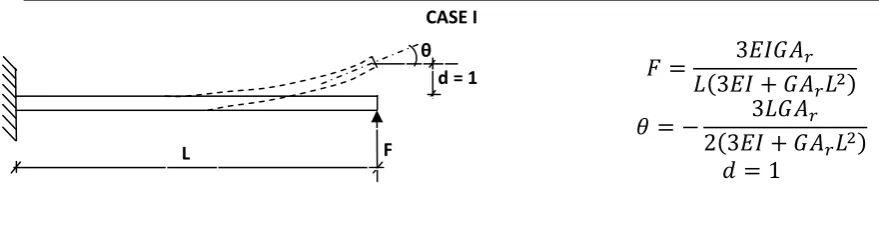
End Forces due to End Displacements of Elements Consider the loaded cantilever of Figure 5 shown below
Using equation (6), d can be evaluated by integration or graphically using a structural engineering table to obtain
3
Since 1
3
3 . .. . . . . . 12
θ can be evaluated by integration or graphically using the structural engineering table to obtain 2 . . . . . . . . . 13
By substituting equation (12) into (13) 3
2 3 . . . . . . . . 14 From fig 5 and equations (12) and (14) Case 1 is developed
F
d = 1
θ
L
Figure 5: A cantilever bar displaced by a unit distance at its end due to the application of a transverse force F
M2
L
w
F1 F2
M
L
a b
M
F2
3
3
3
2 3
1
1
CASE I
Please note that upward forces and displacement were considered positive and clockwise moment and rotation positive.
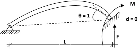
Consider a cantilever with an applied moment at its end as shown in Figure 6 below
Using equation (6), θ can be evaluated by integration or graphically using a structural engineering table to obtain
But since 1
. . . .. . . (15)
Using equation (6), d can be evaluated by integration or graphically using a structural engineering table to obtain
2 . . . . . . . . 16 By substituting the value of M in equation (15) into the equation (16) above
. . . (17)
From Figure 6 and equations (15) and (17) Case II is developed.
CASE II
Consider a propped cantilever rotated through a unit angle at the fixed end as shown in Fig 7 below
d L
θ = 1 M
d L
θ = 1 M
Figure 6: A cantilever bar diplaced by a unit angle at its end due to the application of a moment M
F
d = 1 θ
Using equation (6), θ can be evaluated by integration or graphically using a structural engineering table to obtain 3
1
But since 1
3 . . . . (18)
From Figure 7 and equation (18) Case III is developed
CASE III
For linear elastic structures, stress is linearly proportional to strain ie stress over strain is a constant provided the stress is within the elastic limit of the material. Assuming the deformations are very small, then the law of superposition holds. This implies that an addition of two or more cases will provide another valid case.
Let
CASE IV
3
3
3
2 3
3
3
4 0
Let
M
F θ= 1
L
d = 0 M
F
θ= 1
L
d = 0
Figure 7: A propped cantilever rotated through a unit angle at the fixed end
3
3
1
CASE V
3 4
12
6
3
1 0
Let
CASE VI
3 4
12
0
3
12
4
Let
CASE VII
6
12
4 3
12
0 1
Table 2: End forces caused by end displacement of prismatic members putting shear deformation into consideration.
S/No Beam Force Remark
1 12
12 12 1 1 6 12 6 1 1 See
Case V
2 6
12 6 1 1 2 6 12 2 1 4 3 12 4 1 See
Case VII
3 3
3 12 1 4 3 3 12 1 4 See
Case I
4 3
3 12 1 4 3 3 12 1 4 See
Case III
Where EI is the flexural rigidity, G is the modulus of elasticity in shear
∝ . . . . . . (19)
When dealing in three dimensions
∝ . . . . . (20)
∝ . . . . . (21) Stiffness Matrix of a Space Element
Having obtained the table of the end forces caused by end displacement of prismatic members considering shear deformation the stiffness matrix of equation (6) is evaluated using table 2. The non-zero stiffness coefficients are
, , 12 1
∝ 1
d = 1 M2
M1
F2
F1
L
M2
M1
F1 F2
θ = 1
L
M
F1 F2
d = 1
L
F1
M
F2
θ = 1
3 1
∝ 1 ,
12 1
∝ 1 ,
6 1
∝ 1
12 1
∝ 1 ,
3 1
∝ 1 ,
12 1
∝ 1
6 1
∝ 1 , , ,
∝ 4
∝ 1
6 1
∝ 1 ,
2 ∝
∝ 1 ,
∝ 4
∝ 1
6 1
∝ 1 ,
2 ∝
∝ 1 ,
12 1
∝ 1 ,
6 1
∝ 1 ,
12 1
∝ 1
6 1
∝ 1 , ,
∝ 4
∝ 1
∝ 4
∝ 1
(a) When the Near End is hinged
When the near end is hinged; 0 , because the moments at near end is zero. Consequently
⋯ 0
⋯ 0
⋯ 0
From Table 2 each stiffness coefficent can be deduced. The non-zero ones are
, , 12 1
∝ 4 ,
12 1
∝ 4
12 1
∝ 4 ,
12 1
∝ 4 ,
12 1
∝ 4 ,
12 1
∝ 4
, 12 1
∝ 4 ,
12 1
∝ 4
12 1
∝ 4 ,
12 1
∝ 4
12 1
∝ 4 ,
12 1
∝ 4
By substituting these stiffness coefficents into equation (6) the stiffness matrix (taking shear deformation into account) of a space element hinged at the near end is obtained.
(b) When the Far End is hinged
When the far end is hinged; 0 , because the moments at far end is zero. Consequently
⋯ 0
⋯ 0
⋯ 0
From Table 2 each stiffness coefficent can be deduced. The non-zero ones are
, , 12 1
∝ 4 ,
12 1
∝ 4
12 1
∝ 4 ,
12 1
∝ 4 ,
12 1
12 1
∝ 4 ,
, 12 1
∝ 4 ,
12 1
∝ 4 ,
12 1
∝ 4
12 1
∝ 4 ,
12 1
∝ 4 ,
12 1
∝ 4
By substituting these stiffness coefficents into equation (6) the stiffness matrix (taking shear deformation into account) of a space element hinged at the far end is obtained.
Stiffness Matrix of a Plane Element
For prismatic elements that lie and deform only in one plane, only six degrees of freedom exist (see figure 3.5). If the plane element is lying in the xy plane (see figure 3.5) and all the external loads on it act in the same plane then
0
If the deformation in these coordinates is zero then the forces (or moments for rotations) in these coordinates will also be zero.
0
If these are substituted into equation (1) it will lead to automatic deletion of rows and columns 3, 4, 5, 9, 10 and 11. Equation (8) reduces to
0 0
0 12 1
∝ 1
6 1
∝ 1
0 6 1
∝ 1
∝ 4 ∝ 1
0 0
0 12 1
∝ 1
6 1
∝ 1
0 6 1
∝ 1
2 ∝ ∝ 1
0 0
0 12 1
∝ 1
6 1
∝ 1
0 6 1
∝ 1
2 ∝ ∝ 1
0 0
0 12 1
∝ 1
6 1
∝ 1
0 6 1
∝ 1
∝ 4 ∝ 1
. . . . (22)
, ∝ ∝
Equation (22) is the stiffness matrix of a plane element taking into account deformation due to shear.
a) When the Near End is hinged
0
By substituting these into equaation (1) the stiffness matrix of equation (8) reduces to
∝ ∝ ∝ ∝ ∝ ∝ ∝ ∝
. . . (23)
b) When the Far End is hinged
0
By substituting these into equaation (1) the stiffness matrix of equation (8) reduces to
∝ ∝
∝ ∝
∝
∝
∝ ∝
∝
. (24)
Equation (24) is the stiffness matrix of a plane element hinged at the far end (taking into consideration deformation due to shear).
Summary and Conclusion
Shear deformation is often ignored in structural analysis. The development of the ‘fixed end moments on transversely loaded prismatic elements’ and ‘The end forces due to unit end displacements of prismatic elements’ and which are presented in tables 1 and 2 would facilitate an easy implementation of the deformation due to shear in structural analysis of frames. The component in these tables that captures the effect or contribution deformation due to shear is α.
∝ 12 . . . . 19
Recall that modulus of elasticity in shear is the ratio of shear stress to shear strain . . . 23
Where t is the shear stress and γ is the shear strain.
It then follows that when shear deformation is ignored γ is taken as zero (γ = 0) and the modulus of elasticity in shear G from equation (23) tends to infinity ( ∞ ). If this value of G is substituted into equation (22), ∝ 0 and the forces in table 1 and 2 become the same as that which can be found in many structural engineering textbooks e.g. Davison and Owens (2007) and Reynolds and Steedman (2001).
REFERENCES
[1] Ugural A. C., Fenster S. K. Advanced Strength and Applied Elasticity, 4th Edition, Prentice-Hall Inc New Jersey 2003. [2] Davison B., Owens G. W., Steel Designer’s Maual, 6th Edition, Blackwell Publishing Ltd, UK, 2007
[3] Gere, J. M. Mechanics of Materials. Sixth Edition, Brooks/Cole-Thomson Learning, United States of America. 2004
[4] Ghali A, Neville A. M. Structural Analysis: A Unified Classical and MatrixApproach. 3rd Edition. Chapman & Hall London, 1996 [5] Hibbeler, R. C. Structural Analysis. Sixth Edition, Pearson Prentice Hall, New Jersey. 2006
[6] Jenkins, W. M.,(1990). Structural Analysis using computers. First edition, Longman Group Limited, Hong Kong [7] Leet, K. M., Uang, C., Fundamental of Structural Analysis. McGraw-Hill New York. 2002
[8] Megson T. H. G., Structural and Stress Analysis, 2nd Edition, Elsevier Butterworth-Heinemann, Oxford. 2005
[9] Narayanan, R., Introduction to Manual and Computer Analysis: Steel Designer’s Manual Sixth Edition, Blackwell Science Ltd, United Kingdom. 2007
[10] Nash, W., Schaum’s Outline of Theory and Problems of Strength ofMaterials. Fourth Edition, McGraw-Hill Companies, New York. 1998
[11] Reynolds, C. E.,Steedman J. C. Reinforced Concrete Designer’sHandbook , (10th Edition) E&FN Spon, Taylor & Francis Group, London. 2001
2
1
6
8
7
12
N
F
Figure 2: A 2D representation of the six degrees of freedom (coordinates) of a plane element in the xy plane
Figure 1
1
y
x
z
5
2
4
3
6
11
8
7
10
9
12
(b) A space element showing the twelve
coordinates or degrees of freedom
represented with numbers
d
xNy
x
z
θ
yNd
yNθ
xNd
zNθ
zNθ
yFd
yFd
xFθ
xFd
zFθ
zF(a) A space element showing the twelve
coordinates or degrees of freedom all
labelled appropriately. ‘d’ is for translation
L
w
(c)
(b)
Lw
P
L
a b