https://doi.org/10.5194/cp-15-1427-2019 © Author(s) 2019. This work is distributed under the Creative Commons Attribution 4.0 License.
Impact of different estimations of the background-error
covariance matrix on climate reconstructions
based on data assimilation
Veronika Valler1,2, Jörg Franke1,2, and Stefan Brönnimann1,2
1Institute of Geography, University of Bern, Bern, Switzerland
2Oeschger Centre for Climate Change Research, University of Bern, Bern, Switzerland
Correspondence:Veronika Valler (veronika.valler@giub.unibe.ch)
Received: 4 December 2018 – Discussion started: 20 December 2018 Revised: 5 June 2019 – Accepted: 26 June 2019 – Published: 2 August 2019
Abstract.Data assimilation has been adapted in paleoclima-tology to reconstruct past climate states. A key component of some assimilation systems is the background-error covari-ance matrix, which controls how the information from ob-servations spreads into the model space. In ensemble-based approaches, the background-error covariance matrix can be estimated from the ensemble. Due to the usually limited en-semble size, the background-error covariance matrix is sub-ject to the so-called sampling error. We test different meth-ods to reduce the effect of sampling error in a published paleoclimate data assimilation setup. For this purpose, we conduct a set of experiments, where we assimilate early in-strumental data and proxy records stored in trees, to inves-tigate the effect of (1) the applied localization function and localization length scale; (2) multiplicative and additive in-flation techniques; (3) temporal localization of monthly data, which applies if several time steps are estimated together in the same assimilation window. We find that the estimation of the background-error covariance matrix can be improved by additive inflation where the background-error covariance matrix is not only calculated from the sample covariance but blended with a climatological covariance matrix. Implement-ing a temporal localization for monthly resolved data also led to a better reconstruction.
1 Introduction
Estimating the state of the atmosphere in the past is im-portant to enhance our understanding of the natural cli-mate variability, the underlying mechanisms of past clicli-mate
changes and their impacts. To infer past climate states, two basic sources of information are available: observations and numerical models. Climate models constrained with real-istic, time-dependent external forcings provide fields that are consistent with these forcings and the model physics. Observations can be instrumental meteorological measure-ments, which are mainly available from the mid-19th century. Prior to this time, information from proxies stored in natu-ral archives (like trees, speleothems, marine sediments, ice cores) or documentary data can be exploited. Observations provide important local information; however, their spatial and temporal coverage is sparse.
One popular DA method is the Kalman filter (KF; Kalman, 1960). In standard applications, the processes of the KF can be summarized in two main steps (Ide et al., 1997). In the update step, the background state and the uncertainty of the background state provided by the model simulation are ad-justed by assimilating new observations. In the forecast step, the updated state, called the analysis, and the uncertainty of the analysis are propagated forward in time. These processes are repeated when new observations become available. How-ever, in PDA, the forecast step is usually neglected; that is, the filter is used offline (e.g., Franke et al., 2017a). Because the process is not cycled, the background state is obtained from a precomputed model simulation. In some previous PDA studies, the background state is constructed once from the model simulation, and later, the same state is used in ev-ery assimilation window (Steiger et al., 2018, and references therein); we refer to them as stationary (forcing-independent) offline DA methods. In other PDA studies, the background state is specific for the current assimilation window; that is, the state changes in each assimilation window according to the forcings (Bhend et al., 2012; Franke et al., 2017a); we call them transient (forcing-dependent) offline DA methods. An essential component of the KF is the uncertainty of the background state. In ensemble-based approaches, an ensemble of the background state provides estimation of the truth, represented by the ensemble mean, and the per-turbations from the mean are used to estimate the uncer-tainty, represented by the background-error covariance ma-trix. Ensemble-based KFs are approximations of the KF, be-cause the true state is usually sampled with a few tens to a few hundreds of ensemble members. The limited ensemble size leads to errors in the estimation of the background-error covariance matrix. This effect is known as the sampling error. Two methods are commonly used in online ensemble-based KF approaches to reduce the negative effect of sam-pling error: inflation (e.g., Anderson and Anderson, 1999) and localization (e.g., Hamill et al., 2001) of the background-error covariance matrix. A simple inflation technique is the multiplicative inflation (Anderson and Anderson, 1999), which compensates for potential underestimation of the anal-ysis error. Multiplicative inflation helps to maintain a more realistic distribution of the ensemble members by increas-ing the deviation of the members from the ensemble mean at each DA cycle (Anderson and Anderson, 1999). However, the underestimation of the analysis error is of minor impor-tance in offline approaches, because the ensemble members are not propagated forward in time. Covariance inflation, be-sides reducing the sampling error, can also account for under-estimated model error. In the additive inflation technique, the covariances are inflated by, e.g., adding an additional error term to the background-error covariances (Houtekamer et al., 2005). Covariance localization removes long-range spurious covariances in the background-error covariance matrix that occur by chance due to a limited sample size. Several local-ization techniques have been proposed, from a simple cut-off
radius approach (Houtekamer and Mitchell, 1998) to more sophisticated ones (Houtekamer and Mitchell, 2001; Hamill et al., 2001). By applying covariance localization methods, the elements of the background-error covariance matrix are modified, and in the standard approach the covariances are forced to approach zero at a certain separation length from the location of the observation. This is achieved by multi-plying the background-error covariance matrix element-wise with a distance-dependent function. In practice, this function is often estimated by a Gaussian localization function, rec-ommended by Gaspari and Cohn (1999).
In stationary offline PDA studies, the time-dependent background-error covariance matrix is replaced by a constant covariance matrix (e.g., Steiger et al., 2014). By using a con-stant background-error covariance matrix in the update step, the dependence on the climate state is lost. However, it is pos-sible to estimate the covariance matrix from a much larger ensemble size, which reduces the sampling error. If the con-stant covariance matrix is built from a large enough sample size, representing different climate states, it can be success-fully used in the assimilation process (Steiger et al., 2014).
Covariance inflation and localization techniques are used and under improvement in weather forecasting (e.g., Bowler et al., 2017), but have not yet been sufficiently explored for PDA. In this paper, we discuss three possibilities to im-prove the estimates of background error, relevant to our PDA method:
– The first possibility involves using a two-dimensional multivariate Gaussian function as a horizontal localiza-tion funclocaliza-tion to test the hypothesis of longer correlalocaliza-tion length scales in zonal than meridional direction.
– The second method is by applying covariance infla-tion techniques. In the multiplicative inflainfla-tion tech-nique, a constant factor is used to inflate the deviations from the ensemble mean. In the additive method, the background-error covariance matrix is calculated as the sum of the sample covariance matrix plus a climatolog-ical background matrix, where the climatologclimatolog-ical back-ground is based on all ensemble members of multiple years. This larger sample size decreases the chances of spurious correlations.
– The third possibility is adding temporal localization to the background-error covariance matrix. Multiple time steps are combined in one assimilation window to ef-ficiently assimilate seasonal paleoclimate data. In the case of monthly observations, covariances between the months have been used to update all 6 months (Franke et al., 2017a).
results are presented and each experiment followed directly by a discussion. We summarize our experiments in Sect. 5.
2 Ensemble Kalman fitting framework
2.1 Model simulation: CCC400
We start from an existing DA system, which is described in Bhend et al. (2012) and Franke et al. (2017a). We use the same atmospheric model simulation as in the previous studies. The model simulation, termed as Chemical Climate Change over the Past 400 years (CCC400), has 30 ensemble members that are used as background to reconstruct monthly climate states between 1600 and 2005. Simulations were per-formed with the ECHAM5.4 climate model (Roeckner et al., 2003) at a resolution of T63 with 31 levels in the vertical. The 30 ensemble members were forced and driven with the same external forcings and with the same boundary conditions. For sea-surface temperatures (SSTs), which have a particularly large effect on the simulations, the reconstruction by Mann et al. (2009) was used. At the time when the model simula-tion was run, this was the only available global gridded SST reconstruction that dated back until 1600. The surface tem-perature reconstruction by Mann et al. (2009) is based on a multiproxy network and was produced by a climate field reconstruction method. The SST reconstruction by design captures interdecadal variations (Mann et al., 2009); hence, intra-annual variability dependent on a El Niño–Southern Oscillation reconstructions (Cook et al., 2008) was added to the SST fields. Further forcings include solar irradiance, vol-canic activity and greenhouse gas concentrations (for more details, see Bhend et al., 2012; Franke et al., 2017a). The land-use reconstruction by Pongratz et al. (2008) was used to derive the land-surface parameters. The 6-hourly output fields provided by the model were transformed to monthly means. To reduce the computational burden, only every sec-ond grid point in latitude and longitude was selected. We limit the analysis in this study to 2 m temperature, precipi-tation and sea-level pressure.
2.2 Observational network
In this study, we use the same observational network of tree-ring proxies, documentary data and early instrumental mea-surements as described in Franke et al. (2017a) (Fig. 1), but we only assimilate tree-ring proxies and instrumental data. The temporal resolution of the instrumental air temperature and sea-level pressure measurements is monthly. The tree-ring proxy records have annual resolution. Trees respond to a locally varying growing seasons. We consider temperature from May to August and precipitation from April to June to possibly affect tree-ring width data. The maximum latewood density proxies were considered to be affected by temper-ature over May until August. The observations were qual-ity checked before the assimilation, and outliers which were
more than 5 standard deviations away from the calculated 71-year running mean were discarded, both for instrumental and proxy data.
2.3 Assimilation method
In our paleoclimate reconstruction, we combine the CCC400 model simulation with the observations as described above by implementing a modified version of the ensemble square root filter (EnSRF; Whitaker and Hamill, 2002). This ensemble-based DA method is called ensemble Kalman fit-ting (EKF; Franke et al., 2017a). In fact, the EKF is an of-fline version of the EnSRF, and the update step of the EKF remains the same as of the EnSRF. EKF is described in more detail in Bhend et al. (2012) and Franke et al. (2017a). Here, we shortly highlight the most important aspects of the EKF. The update step in the EnSRF scheme has two parts: updat-ing the mean (x), and for each member, the deviation from the mean (x0). They are calculated as
xa=xb+Ky−Hxb (1)
x0a=x0b+eK
Hx0b, (2)
whereKandeKare
K=PbHTHPbHT+R −1
(3)
e
K=PbHT q
HPbHT +R −1!T
×
q
HPbHT+R+√R −1
. (4)
ob-Figure 1.The observational network in 1904, before the quality check.
Table 1.Defined localization length scale parameters.
Variable Localization length scale (km)
Temperature (2 m) 1500
Precipitation 450
Sea-level pressure 2700
servations can be processed serially. We set the error vari-ances of instrumental temperature observations to 0.9 K2and of instrumental pressure data to 10 hPa2. The error variances are rough estimates that include, for instance, measurement uncertainties, temporal inhomogeneities and the fact that a station is not representative for a grid cell (see Frei, 2014; Franke et al., 2017a). The errors of tree-ring proxy data are calculated as the variance of the multiple regression residu-als of the Hoperator. The assimilation is conducted on the anomaly level: we subtract both from model and from obser-vational data their 71-year running mean in order to deal with the biases related to systematic model errors and inconsistent low-frequency variability in the paleoclimate data.
The use of DA in an offline manner is typical in paleo-climate reconstructions (e.g., Dee et al., 2016). Bhend et al. (2012) argue that the assimilation step is too long for ini-tial conditions to matter, whereas there is some predictabil-ity from the boundary conditions. In addition, Matsikaris et al. (2015) found that both online and offline DA methods perform similarly in their paleoclimate reconstruction setup. Furthermore, the offline DA is advantageous as it allows us-ing the precomputed simulations. In our case, we can use CCC400 (Bhend et al., 2012) and test the method without having to repeat the simulations.
2.4 Spatial localization
AsRis a diagonal matrix, the EKF can be used to assimilate the observations one by one; that is, after the first observation is assimilated and the analysis is obtained, this analysis field becomes the background state for the next observation (see the arrow pointing fromxatoxbon Fig. 2). This serial imple-mentation makes the calculation ofPbsimpler.Hbecomes a vector (not a matrix) of the same length asxb. It is zero ev-erywhere except for a few elements (those required to model the observation). This translates to only a few columns of Pbthat are actually required.HPbHT andRare then scalars (Whitaker and Hamill, 2002). This procedure also makes the localization simpler, as it needs to be applied only to those columns. In the original setup, the elements ofPbwere mul-tiplied (Schur product) with a distance-dependent function (see Eq. 7 in Franke et al., 2017a). For all the variables in the state vector, the same Gaussian function was used but with different localization length scale parameters (Table 1). The localization length scale parameters are defined based on the spatial correlation of the variables in the monthly CCC400 model simulation fields. For the cross-covariances between two variables, the smaller localization length scale of the two variables is applied. With the serial implementation, the cal-culation and localization ofPbis significantly simplified.
3 Experiment design
ex-Figure 2.The main steps of the blending experiment in one assim-ilation window. The blended covariance matrixPblendis calculated as a linear combination from the year specific and climatological covariance matrices. The calculation of the Kalman gain (K) and reduced Kalman gain (eK) matrices is the same as in Eqs. (3) and (4) except the covariance matrix is replaced withPblend. The observa-tion is assimilated to both state vectors and these analysis become to the starting point for assimilating the next observation.
periments are evaluated in terms of performance measures, which then compared to those obtained with the original setup.
3.1 Spatial localization
In most of the studies, the localization function is imple-mented in an isotropic manner. In the original setup, the same horizontally isotropic localization function was used with different localization parameters. However, such spatial sym-metries may not be realistic. In the real atmosphere, correla-tion lengths might be longer in the zonal than in the merid-ional direction, due to the prevailing winds and the weaker large-scale temperature gradients in this direction. On multi-annual to multi-decadal timescales, multiple processes act in the meridional direction, e.g., a widening/shrinking of the Hadley cell, shifts of the Intertropical Convergence Zone or changes in atmospheric modes like the Atlantic Multi-Decadal Oscillation or the North Atlantic Oscillation. These can shift the zonal circulation northward or southward, but the zonal coherence will be less effected. Hence, instead of using a circular Gaussian function, we conducted an experi-ment with a spatially anisotropic localization function
C=exp −1
2 dz2 L2 z
+d
2 m L2 m
!!
, (5)
wheredzanddmare the distances from the selected grid box in the zonal and meridional directions, respectively.Lz and
Lm are the length scale parameters used for localization in the zonal and meridional directions, respectively. As a first experiment, we tested a 2:1 ratio forLz:Lm. We used the values from Table 1 in the meridional direction and doubled them in the zonal direction. Thus, the resulting localization function has an elliptical shape.
3.2 Inflation techniques
Covariance inflation techniques are another possible method to compensate for errors in the DA system (Whitaker et al., 2008). The multiplicative inflation technique uses a small factorγ(γ >1) with which thex0bis multiplied (Anderson and Anderson, 1999). This type of covariance inflation ac-counts for filter divergence due to sampling error (Whitaker and Hamill, 2002) but can be also applied to take into ac-count system errors (Whitaker et al., 2008). We conducted some experiments using multiplicative inflation, although in our offline approach, filter divergence is not the main concern as ensemble members are not propagated in time.
Table 2.Summary of the experiments carried out in this study. The names of the experiments indicate which settings were used in the assimilation. Localization refers to the shape of the localization function applied onPb.γis the multiplicative inflation factor.xclimindicates from how many ensemble members the climatological state vector was constructed.xclimconst stands for keeping the climatological part in the blending experiment unchanged in one October–September time window.Pbloc indicates the localization length scale parameter applied for localizingPb.β2refers to the weight given toPclim.Pclimloc indicates the localization length scale parameter applied for localizing Pclim. i and p stand for instrumental-only and proxy-only observation experiments, respectively.
Name Localization γ Blending Temporal localization Obs. type
xclim xclimconst Pbloc β2(%) Pclimloc
original iso no no i, p
aniso aniso no no i, p
mul1.02 iso 1.02 no i
mul1.12 iso 1.12 no i
25c_PbL_PcL iso no 250 no L 25 L no i, p
50c_PbL_PcnoL iso no 250 no L 50 no no i
50c_PbL_PcL iso no 250 no L 50 L no i, p
50c_PbL_Pc2L_100m iso no 100 no L 50 2L no i
50c_PbL_Pc2L iso no 250 no L 50 2L no i, p
50c_PbL_Pc2L_500m iso no 500 no L 50 2L no i
50c_Pb1.5L_Pc1.5L iso no 250 no 1.5L 50 1.5L no i, p
50c_Pb2L_Pc2L iso no 250 no 2L 50 2L no i, p
75c_PbL_PcL iso no 250 no L 75 L no i, p
75c_PbL_Pc2L iso no 250 no L 75 2L no i, p
75c_PbL_constPc2L iso no 250 yes L 75 2L no i
100c_PcL iso no 250 no 100 L no i, p
100c_constPcL iso no 250 yes 100 L no i
temp_loc iso no yes i
background-error covariance matrix used in the blending ex-periments (Pblend) is built as a linear combination of the sam-ple covariance matrix (Pb) and the climatological covariance matrix (Pclim):
Pblend=β1Pb+β2Pclim, (6)
whereβ1,β2are the weights given to the covariance matri-ces. The sum of the weights is unity.
Figure 2 shows the main steps of the blending assimilation process. First, the covariance matrices were localized sepa-rately; then, we blended them according to the given weights. We conducted several experiments to tune the ratio between the two covariance matrices while using different localiza-tion length scale parameters (L) (Table 2). We used the same Lvalues for localizingPbin most of our experiments to eval-uate improvements in comparison with the original setup. For this study, we calculated the latitudinal dependency of cor-relation of the state variables from a bigger ensemble of the model than in Franke et al. (2017a). The result suggested that longer Lvalues can be applied in the tropics and the Lof precipitation is probably too strict. Based on the rather strict L values in the previous study and the assumption that the covariances can be better estimated from a bigger ensemble, we used doubled length scale parameters (2L) in some of the experiments for localizing the climatological covariances. In this case, the L for temperature is 3000 km, which means
that the correlation is decreased close to zero approximately 6000 km away from the observation.
Since observations are assimilated serially, we also up-datexclim after an observation is assimilated with the same Kalman gain matrices asxb. Thus, in the assimilation pro-cess, we update 30+nensemble members.
3.3 Temporal localization
Localizing observations in time is a special feature of the EKF due to its 6-month assimilation window. Having the state vector in half-year format, every month within the October–March or April–September time window is updated by each single observation. To test whether the covariances between a single observation and the multivariate climate fields are correctly captured, we ran an instrumental-only ex-periment with temporal localization. We set covariances be-tween different months to zero.
3.4 Skill scores
be-tween 1902 and 1959, because many proxy records already end in the 1960s, while the instrumental-only experiments were tested over the 1902–2002 period. We separated the dif-ferent observation types to see whether difdif-ferent settings per-form better depending on the type of data being assimilated. We do not compare proxy-only results with instrumental-only results; hence, the difference in time periods used does not matter; we simply use the longest possible time period. To evaluate the reconstructions, we examined two verifica-tion measures: correlaverifica-tion coefficient and reducverifica-tion of error (RE) skill score (Cook et al., 1994). We use the Climate Re-search Unit (CRU) TS 3.10 dataset (Harris et al., 2014) for reference in the validation process. The presented verifica-tion measures are funcverifica-tions of time. Correlaverifica-tion is calcu-lated between the absolute values of the ensemble mean of the analysis and the reference series at each grid point. The RE compares, in our case, the reconstruction with the model simulation, both expressed as deviations from a reference.
RE=1−
P(xu i −x
ref i )
2
P (xf
i−x ref i )2
, (7)
wherexuis the ensemble mean of the analysis,xfis the en-semble mean of the model background state,xrefis the ref-erence dataset, and i refers to the time step. The RE skill scores are computed based on anomalies with respect to the 71-year running climatologies. Note that xf comes from a forced model simulation; therefore, it already has skill com-pared with a climatological state vector. The RE is 1 if thexu is equal to xref. Negative RE values indicate that the back-ground state is closer to the reference series than the analysis. To test which experiments have significantly different skill compared with the original skill, we carried out a permuta-tion test following the method described in DelSole and Tip-pett (2014). Permutation was performed 10 000 times. If the difference between the median of the experiment and the me-dian of the original data falls outside of the 95 % confidence level of the interval calculated from permuted data, then the experiment is significantly different from the original data.
In the next section, we will focus on analyzing the result of the experiments mainly over the extratropical Northern Hemisphere (ENH), because most of the data are located in this region. The skill scores refer to seasonal averages of the ensemble mean.
4 Results and discussions
4.1 Localization function 4.1.1 Results
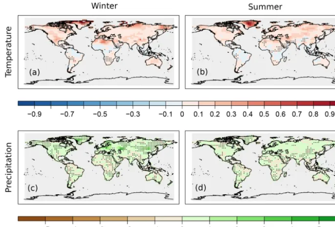
We compared the original setup applying an isotropic local-ization function and the experiment in which an anisotropic localization function was used, to test whether we can obtain a more skillful reconstruction by implementing anisotropic
localization method. As an example of the spatial reconstruc-tion skill, we show the RE values of temperature (Fig. 3). The figures reveal that the type of localization function only resulted in small differences in both experiments. Nonethe-less, there are larger areas of negative RE values (Green-land, Siberia) with the anisotropic localization function in the proxy-only experiment (Fig. 3). In the instrumental-only experiment, the decrease of RE values occur in the north-ern high latitudes and in the Tibetan Plateau in both sea-sons (Fig. 3). To have a better overview of how the skill scores changed, we summarize their distributions with the help of box plots. Figure 4 shows the differences of skill scores between the aniso experiment and the original skill for the three variables (temperature, precipitation and sea-level pressure) in the ENH region. In the instrumental-only exper-iment, correlation values of temperature and sea-level pres-sure decreased in both seasons, while for precipitation they remained mostly unchanged. The RE values show that the experiments with anisotropic localization function reduced the skill of the reconstructions, but the extent of the reduction varies with the variables and with the seasons (Fig. 4). In gen-eral, the same holds for the proxy-only experiment (Fig. 4).
4.1.2 Discussion
In a previous ozone reconstruction study, a seasonally and latitudinally varying localization method was tested which mostly positively affected the analysis (Brönnimann et al., 2013). Here, we increased the zonal distances to see if we can use the information of the observations for a larger re-gion. However, the verification measures are shifted more to the negative direction. We assume that the degraded skill of the reconstruction is due to the choice of too-longLz; hence, spurious correlations were not removed. Using anisotropic localization (doubling theLvalues only in the zonal direc-tion) consistently makes the reconstruction worse.
4.2 Inflation experiments 4.2.1 Results
The main problem of ensemble-based DA techniques is the computationally affordable limited ensemble size. Due to the finite ensemble size, the estimation ofPbsuffers from sam-pling error. Applying inflation techniques is one method to mitigate its effect (see Sect. 3.2).
Figure 3. Spatial skill of temperature reconstruction presented by RE values, assimilating only instrumental data(a, b, d, e)and only proxy records(c, f). Comparing the skill of the reconstruction using isotropic localization function(a–c)versus an anisotropic localization function(d–f). Skill in the winter season(a, d)and in the summer season(b, e, c, f)are shown.
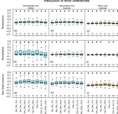
Figure 5.Distribution of correlation coefficients differences between the mixed background-error covariance matrix experiments and the original setup over the ENH region. Panels(a),(d)and(g)show the skill of the reconstruction in the winter seasons, while panels(b),(c),
(e),(f),(h)and(i)show it for the summer season. The labels on thexaxis indicate the experiments. Box plot, color, number and asterisk are the same as in Fig. 4.
RE values slightly decreased (not shown). We did not carry out further experiments since, based on the results, randomly increasing the error in background field did not lead to im-provement.
In the other set of experiments, we usedPblendin the up-date equation (Eq. 6). The experiments were run with using β2equal to 0.25, 0.50, 0.75 and 1 to estimate thePblend (de-noted 25c, 50c, etc.). Besides the varying weight given to Pclim, the appliedLvalues onPbandPclimdiffered as well. ThreeLvalues were used: no localization (termed “no”), ap-plyingLvalues as in Table 1 (L) and doubling these numbers (2L). Different combinations of the fraction ofPclim andL values were termed accordingly (e.g., 50c_PbL_Pc2L).
We expect that estimating the covariances from a bigger ensemble size (n=100–500) instead of 30 members leads
to a more accurate background matrix. In most of our ex-periment,n is 250. Hence,Pclim is likely less affected by the sampling error implying that long-range spurious cor-relations are less prominent, which makes localization less needed. We presume that usingPblendhelps to better recon-struct areas which were characterized with lower skill score values in the original setup and to improve the estimation of unobserved climate variables. The reconstruction skill of the blending experiments is always calculated fromxa(Fig. 2).
Figure 6.Distribution of RE value differences between the mixed background-error covariance matrix experiments and the original setup over the ENH region; otherwise, it is the same as in Fig. 5.
largely reduced, implying that 250 members are not enough to avoid localization altogether (not shown).
Figures 5 and 6 show the distribution of the differences of the skill scores between the experiments and the original analysis for correlation coefficients and RE values, respec-tively. Depending on the variables and the data type being assimilated, different setups perform better. In the case of as-similating only instrumental data, one of the largest increases of median for temperature reconstruction was obtained from the 100c_PcL experiment in both seasons (Figs. 5, 6). Pre-cipitation records were not assimilated; thus, a reasonable estimation of the cross-variable covariances is essential. The skill of the precipitation reconstruction with the original setup, in terms of correlation, is better than the forced simu-lation (not shown); however, the RE values are negative over large regions in the ENH (Fig. 7). Using Pblend in the as-similation, with, e.g., the settings of 50c_PbL_Pc2L
experi-ment, led to more positive RE skill (Fig. 7). The biggest im-provement, in terms of RE skill score, was found in Europe (Fig. 7). The 50c_PbL_Pc2L analysis also has higher skill in North-America, especially in the summer season (Fig. 7). The skill of the sea-level pressure reconstruction also im-proved in the 50c_PbL_Pc2L experiment (Figs. 5, 6). In the proxy-only experiments, 75c_PbL_Pc2L is among the best performing experiments for all the variables (Figs. 5, 6).
en-Figure 7.Spatial reconstruction skill of precipitation in terms of RE values, assimilating only instrumental data. Panels(a)and(b)show the skill of the original setup, and(c)and(d)show the result of the 50c_PbL_Pc2L experiment. The skill in the winter season is presented in panels(a)and(c), and for the summer season in panels(b)and(d).
semble members. An additional experiment was carried out with the same setup but using only 100 ensemble members in the construction ofxclim. The verification measures of the 50c_PbL_Pc2L_100m experiment are higher than the origi-nal one, and the distribution of the skill scores over the ENH region is very similar to what we obtain by using 250 mem-bers inPclimfor temperature and precipitation. However, the sea-level pressure fields from the 50c_PbL_Pc2L experiment have higher skill than those in the 50c_PbL_Pc2L_100m ex-periment (not shown).
Furthermore, we conducted two experiments in which only xbwas updated after an observation was assimilated, and xclim was kept constant in the assimilation window. However, the ensemble members ofxclimwere randomly re-selected for each year (October–September). The advantage of this setup compared to the setup described in Sect. 3.2 is that it is computationally less demanding since only the orig-inal 30 members keep being updated with the observations. In the first test, we giveβ2=0.75 weight toPclim with 2L values. In the second test,β2=1; that is, onlyPclimused for updating xb and theL values in Table 1 were applied for the localization. By comparing the skill of the reconstruc-tions without and with updating the climatological part, we see that the skill scores are higher when the climatological part is also updated with the information from the observa-tions (Fig. 8). The only exception is the correlation values of sea-level pressure: when keeping the climatological part constant, they are slightly higher in both seasons (Fig. 8). Nonetheless, by keeping the climatological part static in one assimilation window, the experiments still outperform the original reconstruction (Fig. 8).
4.2.2 Discussion
We have tested a number of configurations of the mixed co-variance matrixPblendto evaluate the effect of the sampling error. In numerical weather predication (NWP) applications, various methods have been designed to better estimate the errors of the background state. In hybrid DA systems, the advantages of variational and ensemble Kalman filter tech-niques are combined (Hamill and Snyder, 2000; Lorenc, 2003). In another method, the background-error covariances are obtained from an ensemble of assimilation experiments performed by a variational assimilation system (Pereira and Berre, 2006). In an additive inflation experiment, a term is added to thexa to account for the errors of the DA system (Whitaker et al., 2008).
Figure 9.Difference of the RE skill between the temporally localized experiment and the original setup, when only instrumental data are assimilated. Temperature(a, b)and precipitation(c, d)differences are shown in the winter(a, c)and in the summer(b, d)seasons. The black dots indicate the negative RE values in the temporally localized experiment.
tal measurements are assimilated. However, other settings resulted in larger increase of median for different variables and observation types. By applying no localization onPclim in the 50c_PbL_PcnoL experiment, we obtained a less skill-ful reconstruction than by using the other two localization schemes. The skills reduced especially over the areas where no local observations were assimilated. Using 2Lvalues for localizing the covariances ofPclim in the instrumental-only experiments resulted in higher correlation values of sea-level pressure (50c_PbL_Pc2L) and helped to obtain higher corre-lation scores of precipitation in summer. Among the proxy-only experiments, 75c_PbL_Pc2L shows the largest increase of median for pressure reconstruction. Here, pressure data are not assimilated, and the result suggests that by applying longer L values, the cross-variable covariances are treated better. We tested whether the skill of the experiments per-formed with various settings is significantly different from the skill of the original analysis. We compared the median value of the skill scores from the experiments and the origi-nal data, and with most of the settings a significant difference was obtained for all the variables. The results of the experi-ments show that with a mixed covariance matrix implemen-tation, a major drawback of the ensemble-based DA system, due to the limited ensemble size, can be improved.
4.3 Localization in time 4.3.1 Results
Since 6-monthly time steps were combined in one state vec-tor (one assimilation window), covariances between
differ-ent months also need to be considered. An additional exper-iment was conducted in which the (localized)Pbwas multi-plied with a temporal localization function when instrumen-tal data were assimilated. This is a specific experiment due to the structure of EKF. The assimilation window in the EKF is 6 months; hence, a single observation is enabled to ad-just all the meteorological variables inxbin a half-year time window. In the temporal localization experiment, the infor-mation from a given observation can only modify the differ-ent climate fields in its currdiffer-ent month, while leaving all other fields of the 5 months unchanged (Table 2). In general, the skill scores indicate an improvement. The differences of RE values between the temp_loc and original experiments are mostly positive over the northern high-latitude areas (Fig. 9).
4.3.2 Discussion
5 Conclusions
In this study, a transient offline data assimilation ap-proach was used to test the effect of the estimation of the background-error covariance matrix in a climate reconstruc-tion. Several experiments were evaluated with different val-idation measures to see which background-error covariance matrix estimation techniques improve the skill of the recon-struction. The evaluation of the presented techniques sug-gests the following: (1) applying an anisotropic localization function on the sample covariance matrix did not improve the reconstruction; (2) most of the settings, which make use of covariance estimates from a larger climatological sample, result in significantly improved skills compared to an esti-mation from the 30-member ensemble; (3) assimilating early instrumental data with temporal localization leads to a bet-ter analysis. To which extent the different techniques helped in the estimation of the background-error covariance matrix varies geographically and also depends on the climate vari-able being reconstructed. The cross-varivari-able covariances of the background-error covariance matrix can provide infor-mation from unobserved climate variables. Including clima-tological information in the estimation of precipitation has led to a better reconstruction, especially in Europe. Estimat-ing sea-level pressure with the blended Pblend matrix also improved the skill of the reconstruction. For instance, the 50c_PbL_Pc2L experiment performs constantly better than the original setup. This study shows that results can be im-proved by better specifying the background-error covariance matrix. In the future, we will combine all the techniques that lead to more skillful analyses to produce a climate recon-struction over the last 400 years.
Data availability. The EKF400 reanalysis is available at the World Data Center for Climate at Deutsches Klimarechenzen-trum (DKRZ) in Hamburg, Germany (https://cera-www.dkrz.de/ WDCC/ui/cerasearch/entry?acronym=EKF400_v1.1; Franke et al., 2017b). The sensitivity experiments analyzed in this study are available upon request: veronika.valler@giub.unibe.ch, jo-erg.franke@giub.unibe.ch.
Author contributions. All authors were involved designing the study and contributed to writing the paper. VV conducted the ex-periments and performed most of the analyses. JF developed the original code and helped with the analyses.
Competing interests. The authors declare that they have no con-flict of interest.
Acknowledgements. The CCC400 simulation was performed at the Swiss National Supercomputing Centre CSCS. The comments of the two anonymous reviewers are gratefully acknowledged.
Financial support. This research has been supported by the Swiss National Science Foundation (grant no. 162668) and the Eu-ropean Commission – Horizon 2020 (grant no. 787574).
Review statement. This paper was edited by Bjørg Rise-brobakken and reviewed by two anonymous referees.
References
Anderson, J. L. and Anderson, S. L.: A Monte Carlo im-plementation of the nonlinear filtering problem to pro-duce ensemble assimilations and forecasts, Mon. Weather Rev., 127, 2741–2758, https://doi.org/10.1175/1520-0493(1999)127<2741:AMCIOT>2.0.CO;2, 1999.
Bhend, J., Franke, J., Folini, D., Wild, M., and Brönnimann, S.: An ensemble-based approach to climate reconstructions, Clim. Past, 8, 963-976, https://doi.org/10.5194/cp-8-963-2012, 2012. Bowler, N., Clayton, A., Jardak, M., Jermey, P., Lorenc, A.,
Wlasak, M., Barker, D., Inverarity, G., and Swinbank, R.: The effect of improved ensemble covariances on hybrid varia-tional data assimilation, Q. J. Roy. Meteor. Soc., 143, 785–797, https://doi.org/10.1002/qj.2964, 2017.
Brönnimann, S., Bhend, J., Franke, J., Flückiger, S., Fischer, A. M., Bleisch, R., Bodeker, G., Hassler, B., Rozanov, E., and Schraner, M.: A global historical ozone data set and prominent features of stratospheric variability prior to 1979, Atmos. Chem. Phys., 13, 9623–9639, https://doi.org/10.5194/acp-13-9623-2013, 2013. Clayton, A. M., Lorenc, A. C., and Barker, D. M.: Operational
im-plementation of a hybrid ensemble/4D-Var global data assimi-lation system at the Met Office, Q. J. Roy. Meteor. Soc., 139, 1445–1461, https://doi.org/10.1002/qj.2054, 2013.
Cook, E. R., D’Arrigo, R., and Anchukaitis, K.: ENSO recon-structions from long tree-ring chronologies: Unifying the dif-ferences?, talk presented at a special workshop on “Reconciling ENSO Chronologies for the Past 500 Years”, 2–3 April 2008, Moorea, French Polynesia, 2008.
Cook, E. R., Briffa, K. R., and Jones, P. D.: Spatial re-gression methods in dendroclimatology: a review and com-parison of two techniques, Int. J. Climatol., 14, 379–402, https://doi.org/10.1002/joc.3370140404, 1994.
Dee, S. G., Steiger, N. J., Emile-Geay, J., and Hakim, G. J.: On the utility of proxy system models for estimating climate states over the common era, J. Adv. Model. Earth Sy., 8, 1164–1179, https://doi.org/10.1002/2016MS000677, 2016.
DelSole, T. and Tippett, M. K.: Comparing forecast skill, Mon. Weather Rev., 142, 4658–4678, https://doi.org/10.1175/MWR-D-14-00045.1, 2014.
Franke, J., Brönnimann, S., Bhend, J., and Brugnara, Y.: A monthly global paleo-reanalysis of the atmosphere from 1600 to 2005 for studying past climatic variations, Scientific data, 4, 170076, https://doi.org/10.1038/sdata.2017.76, 2017a.
Frei, C.: Interpolation of temperature in a mountainous region using nonlinear profiles and non-Euclidean distances, Int. J. Climatol., 34, 1585–1605, 2014.
Gaspari, G. and Cohn, S. E.: Construction of correlation functions in two and three dimensions, Q. J. Roy. Meteor. Soc., 125, 723– 757, https://doi.org/10.1002/qj.49712555417, 1999.
Gebhardt, C., Kühl, N., Hense, A., and Litt, T.: Recon-struction of Quaternary temperature fields by dynami-cally consistent smoothing, Clim. Dynam., 30, 421–437, https://doi.org/10.1007/s00382-007-0299-9, 2008.
Goosse, H., Renssen, H., Timmermann, A., Bradley, R. S., and Mann, M. E.: Using paleoclimate proxy-data to select op-timal realisations in an ensemble of simulations of the cli-mate of the past millennium, Clim. Dynam., 27, 165–184, https://doi.org/10.1007/s00382-006-0128-6, 2006.
Goosse, H., Crespin, E., de Montety, A., Mann, M., Renssen, H., and Timmermann, A.: Reconstructing surface temperature changes over the past 600 years using climate model simulations with data assimilation, J. Geophys. Res.-Atmos., 115, D09108, https://doi.org/10.1029/2009JD012737, 2010.
Hakim, G. J., Emile-Geay, J., Steig, E. J., Noone, D., An-derson, D. M., Tardif, R., Steiger, N., and Perkins, W. A.: The last millennium climate reanalysis project: Framework and first results, J. Geophys. Res.-Atmos., 121, 6745–6764, https://doi.org/10.1002/2016JD024751, 2016.
Hamill, T. M. and Snyder, C.: A hybrid ensemble Kalman filter – 3D variational analysis scheme, Mon. Weather Rev., 128, 2905–2919, https://doi.org/10.1175/1520-0493(2000)128<2905:AHEKFV>2.0.CO;2, 2000.
Hamill, T. M., Whitaker, J. S., and Snyder, C.: Distance-dependent filtering of background error covariance es-timates in an ensemble Kalman filter, Mon. Weather Rev., 129, 2776–2790, https://doi.org/10.1175/1520-0493(2001)129<2776:DDFOBE>2.0.CO;2, 2001.
Harris, I., Jones, P. D., Osborn, T. J., and Lister, D. H.: Up-dated high-resolution grids of monthly climatic observations– the CRU TS3. 10 Dataset, Int. J. Climatol., 34, 623–642, https://doi.org/10.1002/joc.3711, 2014.
Houtekamer, P. L. and Mitchell, H. L.: Data assimila-tion using an ensemble Kalman filter technique, Mon. Weather Rev., 126, 796–811, https://doi.org/10.1175/1520-0493(1998)126<0796:DAUAEK>2.0.CO;2, 1998.
Houtekamer, P. L. and Mitchell, H. L.: A sequential ensem-ble Kalman filter for atmospheric data assimilation, Mon. Weather Rev., 129, 123–137, https://doi.org/10.1175/1520-0493(2001)129<0123:ASEKFF>2.0.CO;2, 2001.
Houtekamer, P. L. and Mitchell, H. L.: Ensemble Kalman filtering, Q. J. Roy. Meteor. Soc., 131, 3269–3289, https://doi.org/10.1256/qj.05.135, 2005.
Houtekamer, P. L., Mitchell, H. L., Pellerin, G., Buehner, M., Charron, M., Spacek, L., and Hansen, B.: Atmospheric data assimilation with an ensemble Kalman filter: Results with real observations, Mon. Weather Rev., 133, 604–620, https://doi.org/10.1175/MWR-2864.1, 2005.
Ide, K., Courtier, P., Ghil, M., and Lorenc, A. C.: Unified Notation for Data Assimilation: Operational, Sequential and Variational, J. Meteorol. Soc. Jpn. Ser. II, 75, 181–189, https://doi.org/10.2151/jmsj1965.75.1B_181, 1997.
Kalman, R. E.: A new approach to linear filtering and prediction problems, J. Basic Eng.-T. ASME, 82, 35–45, 1960.
Lorenc, A. C.: The potential of the ensemble Kalman filter for NWP—a comparison with 4D-Var, Q. J. Roy. Meteor. Soc., 129, 3183–3203, https://doi.org/10.1256/qj.02.132, 2003.
Mann, M. E., Zhang, Z., Rutherford, S., Bradley, R. S., Hughes, M. K., Shindell, D., Ammann, C., Faluvegi, G., and Ni, F.: Global signatures and dynamical origins of the Little Ice Age and Medieval Climate Anomaly, Science, 326, 1256–1260, https://doi.org/10.1126/science.1177303, 2009.
Matsikaris, A., Widmann, M., and Jungclaus, J.: On-line and off-line data assimilation in palaeoclimatology: a case study, Clim. Past, 11, 81–93, https://doi.org/10.5194/cp-11-81-2015, 2015. Pereira, M. B. and Berre, L.: The use of an ensemble
ap-proach to study the background error covariances in a global NWP model, Mon. Weather Rev., 134, 2466–2489, https://doi.org/10.1175/MWR3189.1, 2006.
Pongratz, J., Reick, C., Raddatz, T., and Claussen, M.: A re-construction of global agricultural areas and land cover for the last millennium, Global Biogeochem. Cy., 22, GB3018, https://doi.org/10.1029/2007GB003153, 2008.
Roeckner, E., Bäuml, G., Bonaventura, L., Brokopf, R., Esch, M., Giorgetta, M., Hagemann, S., Kirchner, I., Kornblueh, L., Manzini, E., Rhodin, A., Schlese, U., Schulzweida, U., and Tompkins, A.: The atmospheric general circulation model ECHAM5 Part I: model description, Tech. rep. 349, Max Planck Institute for Meteorology, 2003.
Steiger, N. J., Hakim, G. J., Steig, E. J., Battisti, D. S., and Roe, G. H.: Assimilation of time-averaged pseudo-proxies for climate reconstruction, J. Climate, 27, 426–441, https://doi.org/10.1175/JCLI-D-12-00693.1, 2014.
Steiger, N. J., Smerdon, J. E., Cook, E. R., and Cook, B. I.: A reconstruction of global hydroclimate and dynamical vari-ables over the Common Era, Scientific Data, 5, 180086, https://doi.org/10.1038/sdata.2018.86, 2018.
Whitaker, J. S. and Hamill, T. M.: Ensemble data assimi-lation without perturbed observations, Mon. Weather Rev., 130, 1913–1924, https://doi.org/10.1175/1520-0493(2002)130<1913:EDAWPO>2.0.CO;2, 2002.
Whitaker, J. S., Hamill, T. M., Wei, X., Song, Y., and Toth, Z.: Ensemble data assimilation with the NCEP global forecast system, Mon. Weather Rev., 136, 463–482, https://doi.org/10.1175/2007MWR2018.1, 2008.