978-1-4577-0351-5/11/$26.00 c2011 IEEE
Power save analysis of cellular networks with continuous connectivity
Vincenzo Mancuso Institute IMDEA Networks
Madrid, Spain
Email: [email protected]
Sara Alouf
INRIA Sophia Antipolis M´editerran´ee Sophia Antipolis, France Email: [email protected]
Abstract—In this paper, we analyze the power save and its
impact on web traffic performance when customers adopt the continuous connectivity paradigm. To this aim, we provide a model for packet transmission and cost. We model each mobile user’s traffic with a realistic web traffic profile, and study the aggregate behavior of the users attached to a base station by means of a processor-shared queueing system. In particular, we evaluate user access delay, download time and expected economy of energy in the cell. The model is validated through packet-level simulations. Our model shows that dramatic energy save can be achieved by both mobile users and base stations, e.g., as much as 70% of the energy cost due to packet transmission at the base station.
Keywords-power saving; cellular network; analytical model;
I. INTRODUCTION
The total operating cost for a cellular network is of the order of tens of millions of dollars for a medium-small network with twenty thousand base stations [1]. A relevant portion of this cost is due to power consumption, which can be dramatically reduced by using efficient power save strategies. Power save can be achieved in cellular networks operating WiMAX, HSPA, or LTE protocols by optimizing the hardware, the coverage and the distribution of the signal, or also by implementing energy-aware radio resource management mechanisms. In particular, we focus on power save in wireless transmissions, which would enable the deployment of compact (e.g., air conditioning free) and green (e.g., solar power operated) base stations, thus requiring less operational and management costs.
An interesting case study is offered by the behavioral analysis of users that remain online for long periods. These users request a continuous availability of a dedicated wide-band data channel, in order to shorten the delay to access the network as soon as new packets have to be exchanged. This continuous connectivity requires frequent exchange of control packets, even when no data are awaiting for transmission. Therefore, in case of continuous connectivity, a huge amount of energy might be spent just to control the high-speed connection, unless power save is enforced. However, since power save mode affects packet delay, some
This work was supported in part by the WiNEM project (funded by ANR RNRT 2006), the ICT FLAVIA Project (funded by the EU Framework 7 Programme), and the MEDIANET Project (grant S2009/TIC-1468) from the General Directorate of Universities and Research of the Regional Government of Madrid.
constraints have to be considered when turning to the power save operational mode.
Power save and sleep mode in cellular networks have been analytically and experimentally investigated in the literature, mainly from the user equipment (UE) viewpoint. E.g., power save in the UMTS UE has been evaluated in [2] and [3] by means of a semi-Markov chain model. The authors of [4] proposed an embedded Markov chain to model the system vacations in IEEE 802.16e, where the base station queue is seen as an M/GI/1/N system. In [5], the authors use an M/G/1queue with repeated vacations to model an 802.16e-like sleep mode and to compute the service cost for a single user download. Analytical models, supported by simulations, were proposed by Xiao for evaluating the performance of the UE in terms of energy consumption and access delay in both downlink and uplink [6]. The authors of [7] provide an adaptive algorithm that minimizes energy subject to QoS requirements for delay.
The existing work does not tackles the base station (or evolved node B, namely eNB) viewpoint nor analytically captures the relation between cell load and service rate statistics. Furthermore, for sake of tractability, many of those studies assume that packet arrivals follow a Poisson model. Instead, in real networks, the user traffic can be very bursty and follow long tail distributions [8]. In contrast, we use a G/G/1queue with vacations to model the behavior of each UE, and we compose the behavior of multiple users into a single G/G/1P S queue that models the eNB traffic. We analytically compute the cost reduction achievable thanks to power save mode operations, and show how to minimize the system cost under QoS constraints. In particular we refer to the mechanisms made available by 3GPP forContinuous Packet Connectivity(CPC), i.e., the discontinuous transmis-sion (DTX) and discontinuous reception (DRX) [9].
The importance of DRX has been addressed in [10], where the authors model a procedure for adapting the DRX parameters based on the traffic demand, in LTE and UMTS, via a semi-Markov model for bursty packet data traffic. A description of DRX advantages in LTE from the user viewpoint is given in [11] by means of a simple cost model. In [12], the authors use heuristics and simulation to show the importance of DRX for the UE.
and with non-Poisson traffic, (ii)we provide a cost model that incorporates the different causes of operational costs, and (iii) we show how to use the model to minimize operational costs under QoS constraints. Our model has been validated through packet-level simulations, and our results confirm that a tremendous cost reduction can be attained by correctly tuning the power save parameters. In particular, eNB transmission costs can be lowered by more than 70%. The paper is organized as follows: Section II presents power save operations in continuous connectivity mode; Section III describes a model for cellular users generating web traffic. Section IV illustrates a model for downlink transmissions, and Section V describes how to evaluate flow performance and transmission costs. In Section VI we validate the model through simulation, and show the achievable power saving. Section VII concludes the paper.
II. CONTINUOUS CONNECTIVITY
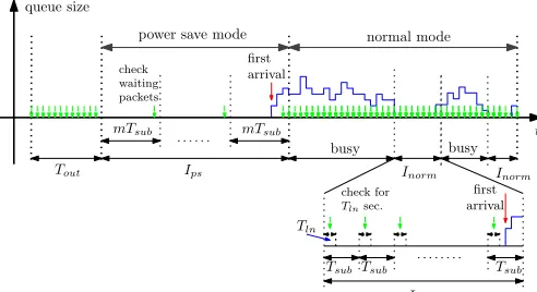
Cellular packet networks, in which the base station sched-ules the user activity, require the online UEs to check a control channel continuously, namely for Tln seconds per system slot (i.e., per subframeTsub). For instance, CPC has been defined by 3GPP for the next generation of high-speed mobile users, in which users register to the data packet service of their wireless operator and then remain online even when they do not transmit or receive any data for long periods [13]. A highly efficient power save mode operation is then strongly required, which would allow disabling both transmission and reception of frames during the idle periods. The UE, however, has to transmit and receive control frames at regular rhythm, every few tens of milliseconds, so that synchronization with the base station and power control loop can be maintained. Therefore, idle periods are limited by the mandatory control activity that involves the UE. To save energy, when there is no traffic for the user, the UE can enter a power save mode in which it checks and reports on the control channels according to a fixed pattern, i.e., only once everym time slots. Relevant energy economy can be achieved. In change, the queued packets have to wait for the mth subframe before being served.
Discontinuous transmission.DTX has been first defined
by 3GPP release 7. It is a UE operational mode for dis-continuous uplink transmission over the Dedicated Physical Control Channel (DPCCH). With DTX, UEs transmit control information according to a cycle. There are actually two possible DTX cycles. The first cycle is used when some data activity is present in the uplink (normal operation), and it is a short cycle (one or very few subframes). The second cycle is longer (up to tens of subframes), and is triggered after an inactivity timeout in the uplink data channel expires (power save mode operation). The thresholdM for inactivity period is a power of 2 subframes. Since transmissions on uplink data channel can only start in parallel with DPCCH transmissions, DTX also regulates data transmissions.
Tout
mTsub mTsub
busy
Ips
Inorm
Tsub
power save mode queue size
t
first arrival
check waiting packets
Inorm
busy
Inorm
normal mode
Tsub Tsub
first arrival
Tln
check for
Tlnsec.
Figure 1. Downlink queue activity with power save and normal operation.
Discontinuous reception. DRX is an operational mode
defined by 3GPP release 6 for the UE to save energy while monitoring the control information transmitted by the eNB. It also affects data delivery, since no data can be dependably received without an associated control frame. 3GPP specifications define a cycle, that is the total number of subframes in a listening/sleeping window out of which only one subframe is used for control reception. Valid values for this cycle are 4 to 20 subframes (i.e., using a 2 ms subframe in HSPA yields a cycle of 8 to 40 ms). DRX is activated only upon a timeout expiry after the last downlink transmission, and like DTX, the timeout threshold specified in the standard isM subframes, withM being a power of 2.
III. POWER SAVE MODEL
We focus on the power consumption due to wireless activity on the air interface of mobile users (UEs) and base station (eNB). On the one hand, we assume that uplink control transmission follows the DTX pattern. On the other hand, the UE has to decode the downlink control channel according to the DRX pattern, and receive packets accordingly [13]. Thus, uplink power save can be enabled by means of a long DTX cycle, with a timeout whose duration can be of the same order of the subframe size. Downlink power save is similarly enforced by setting the DRX cycle and timeout.
Thereby, power save issues in uplink and downlink can be modeled in a similar way, and there is little difference between the cost computation of a single UE and the one of a base station. In fact, the evaluation of the costs at the eNB, can be seen as the collection of costs over the control and data channels towards the various UEs, plus a fixed per-cell operational cost that the eNB has to pay to notify its presence and maintain the users synchronized. Therefore, here we focus on the downlink only, and begin our analysis with the behavior of a UE receiving a data stream.
Power save in downlink. As illustrated in Figure 1,
mode); instead, upon the expiration of an inactivity timeout Tout, consisting of M subframes, there is a longer cycle in which the UE checks the control channel periodically, with periodmsubframes (power save mode).1In power save mode, the UE samples the downlink control channel every m subframes, and returns to normal mode as soon as the channel sampling detects a control message indicating that the downlink queue is no longer empty. Note that UEs do not receive any service during:(i)Inorm, i.e., idle intervals in normal operation,(ii)timeout intervals, and(iii)Ips, i.e., idle intervals in power save mode.
To quantify the power save that can be achieved at the UE, in Section IV we model the behavior of downlink transmissions with DRX operations enabled and users gen-erating web traffic. Then, in Section V we discuss the tradeoff between per-packet performance and per-UE cost. Our model can be used for systems using slotted operations, and in particular LTE and HSPA [13]. The model can be applied to both uplink and downlink. However, for sake of clarity, we explicitly deal with the downlink case.
Achievable cost saving and performance metrics will be expressed as a function of the subframe length Tsub and the DRX parameters, namely the timeout duration, through the parameterM, and the DRX power save cycle duration, through the parameterm. We assume fixed-length packets, and the server capacity is exactly one packet per subframe. However, no packet is served for UEs in power save mode, and the server capacity is shared, in each subframe, between the UEs operating in normal mode. Therefore, we model a system which behaves as aG/G/1P Squeue with repeated fixed-length vacations ofmTsub seconds.
Before proceeding with the model derivation, we intro-duce the traffic model adopted in this study.
Traffic model. We assume that downlink traffic is the
composition of users’ web browsing sessions. Traffic profile is the same for all users and is as follows. The size of each web request is modeled as suggested by 3GPP2 in [14]: a web page consists of one main object, whose size is a random variable with truncated lognormal distribution, and zero or more embedded objects, each with random, truncated lognormal distributed size. The number of embed-ded objects is a random variable derived from a truncated Pareto distribution. Each web page request triggers the download of the packets carrying the main object only. Then a parsing time is needed for the user application to parse the main object and request the embedded objects, if any. The parsing time distribution is exponential with rate λp. After having received the last packet of the last object, the customerreadsthe web page for an exponentially distributed
1The actual system timeout isM-subframe long. However, since the UE
checks for new traffic at the beginning of a subframe, the UE switches to power save mode if it does not receive any traffic alert at the beginning of theMth idle subframe. Therefore, it is enough to have no arrivals for M−1subframes and the UE will not receive any packet forMsubframes.
embedded object(s)
t
first arrival
main object parsing reading
access delay access
delay
queue size
system cycle (web page)
busy busy
Figure 2. System cycle with web traffic as defined in [14].
reading time, whose rate is λr. If no object is embedded, the reading time includes the parsing time. Finally he/she requests another web page. Figure 2 represents the UE’s downlink queue size at the eNB during a generic web page request and download. Table I summarizes the parameters used for the generation of web browsing sessions. Note that the probability ψ0 to have no embedded objects in a
web page can be computed through the distribution of the truncated Pareto random variable Y described in Table I: ψ0 = P(ymin ≤ Y < ymin+ 1) = 1−
ymin
ymin+1
α
. Note also that the downlink of the web page experiences a small access delay due to the completion of the current DRX cycle before the first packet of the new burst could be served.
In our model, we assume that the time to request a web object with an http GET command is negligible in comparison with the time needed to parse the main object, and therefore also in comparison with the time needed for a customer to read the web page. Hence we incorporate this request delay in the parsing time and in the reading time. In this way, we clearly focus our study on the sole impact of the wireless technology on the system performance and costs. Furthermore, packet arrivals are supposed to be bursty after each GET request, so that no power save mode can be triggered after an object download begins, i.e., all power save intervals are contained in either parsing or reading times. With these assumptions, we study the system performance through the analysis of a generic web page download and its fruition. More precisely, we study the system cycle defined as the time in between two consecutive web page requests. Therefore, the system cycle can be decomposed in four phases, as depicted in Figure 2:(i) download of the main object of the web page,(ii)parsing of the main object,(iii) download of embedded objects, and(iv)web page reading. The first three phases represent the web page download time, from the first packet arrival in the eNB queue to the last packet delivery to the UE. Access delay and download time characterize the service experienced by the customer.
IV. MODEL DERIVATION
Here we derive the time spent by the system in the various cycle phases. For ease of notation, we defineβp=e−λpTsub andβr=e−λrTsub as the probabilities that, respectively, the exponentially distributed parsing time and reading time are longer than one subframe. Hence the timeout probability is βM−1
Table I
PARAMETERS SUGGESTED BY3GPP2FOR THE EVALUATION OF WEB TRAFFIC
Quantity Derivation Probability distribution Parameters
Main object size Smo=⌈X⌉ fX(x) =
2πσ2
X −12e−
(lnx−µX)2
2σ2X
Z xmax
xmin 2πσ2X
−12e−
(lnt−µX)2
2σ2 X dt
µX= 8.35,σX= 1.37,
x∈[xmin, xmax] xmin= 100bytes,xmax= 2·106bytes
Number of embedded objects Neo=⌊Y⌋ −ymin fY(y) =α yα
min
yα+1, y∈[ymin, ymax[ ymin= 2,ymax= 55
fY(ymax) =1− yymin
max
α
δ(y−ymax) α= 1.1
Embedded object size Seo=⌈Z⌉ fZ(z) =
2πσ2
Z −12e−
(lnz−µZ)2
2σ2 Z
Z zmax
zmin 2πσ2Z
−12e−
(lnt−µZ)2
2σ2 Z dt
µZ= 6.17,σZ= 2.36,
z∈[zmin, zmax] zmin= 50bytes,zmax= 2·106 bytes
Reading time Λr fΛr(t) =λre−λrt,t≥0 λr= 0.03
Parsing time Λp fΛp(t) =λpe−
λpt,t≥0 λp= 7.69
Timeouts in a cycle. Each cycle always includes one
reading time, while the parsing time is present with probabil-ity1−ψ0, i.e., only if there are embedded objects. Therefore,
the average number of timeouts in a system cycle is:
E[Nto] =βrM−1+ (1−ψ0)βMp −1. (1)
Hence each cycle includes, on average,E[Nto](M−1)Tsub seconds due to timeout occurrences.
Idle time in power save mode. The average time per
cycle during which the system is in power save mode, denoted asI0, is computed by summing up the time spent in
power save mode (the intervalsIpsas in Figure 1) occurring in the reading time and in the parsing time, if any is present in the cycle: I0 = Ips|reading +Ips|parsing. Thanks to the
memoryless property of exponential arrivals, the interval between the timeout expiration and the arrival of the next data packet is exponential too, and has the same exponential rate. In particular, the power save interval that begins in the reading time lasts a multiple number of checking intervals mTsub, with the following distribution and average:
P(I0=jmTsub|reading timeout)
=P(0 arrivals in(j−1)mTsub)[1−P(0 arrivals in mTsub)] = (βmr )
j−1
(1−βmr ), j≥1; E[I0|reading] =βrM−1
mTsub 1−βm
r
; (2)
where we also removed the conditioning on the timeout occurrence. Similarly, for the parsing time:
E[I0|parsing] =βpM−1 mTsub 1−βm
p
. (3)
Therefore, the expected value of the time spent in power save mode in a system cycle is given by the following average:
E[I0] =βrM−1 mTsub 1−βm
r
+ (1−ψ0)βMp −1 mTsub 1−βm
p
. (4)
Note that E[I0] is a function of m andM, the web traffic
parameters being fixed. It is easy to find that ∂m∂ E[I0]>0,
and ∂M∂ E[I0] < 0, hence the power save interval I0
monotonically grows with the duration of the DRX cycle, and decreases with the duration of the timeout.
Idle time in normal mode. The amount of time spent
in normal mode without serving any traffic is the sum of the normal mode idle intervals due to parsing and reading times. Since we counted apart the time spent in timeouts by means of (1), here we only count the intervalsInorm, whose sum over a system cycle is denoted byI1=Inorm|reading+
Inorm|parsing. Considering thatInorm is always a multiple of Tsubbut smaller than a timeout, and since the component of I1in reading time isInorm|reading, the conditional distribution
ofI1 in reading time is as follows:
P(I1=jTsub|reading)
= P(Inorm=jTsub|exp. arrivals with rate λr)
=
(
βM−1
r j= 0;
βj−1
r (1−βr) 1≤j ≤M −1.
Hence the conditional expected value of this intervalI1 is:
E[I1|reading] =Tsub
1−M βM−1
r + (M−1)βMr 1−βr
. (5)
Similarly, the expected value for the time spent in normal mode with no traffic to be served during parsing, without counting the timeout, is given by
E[I1|parsing] =Tsub
1−M βM−1
p + (M −1)βpM 1−βp
. (6)
Therefore, on average, the time spent in normal mode without serving any traffic during a system cycle is given by the timeout intervals plusE[I1|reading], plus 1−ψ0 times
E[I1|parsing]. So, the expected value of I1 increases with
Cumulative idle time. The cumulative amount of idle time I in a cycle is the sum of timeouts, I0, and I1. Its
expected value is then as follows:
E[I] = βrM−1 mTsub 1−βm
r
+Tsub
1−βM−1
r 1−βr
+(1−ψ0) βpM−1 mTsub 1−βm p
+Tsub
1−βM−1
p 1−βp
!
. (7)
E[I]is a decreasing function ofM, and increases with m. However, with our model assumptions,E[I]is slightly larger than the sum of reading and parsing times. More precisely, its value is bounded as follows:
1 λr
+1−ψ0 λp
< E[I]< 1 λr
+mTsub+(1−ψ0)
1 λp
+mTsub
.
Given that m can be as high as few tens, and Tsub is only few milliseconds, the product mTsub is negligible in comparison with the average parsing and reading times. Hence, for all realistic values ofm, the per-cycle idle time can be considered constant and equal to its lower bound.
Busy time.The expected time spent to serve the packets
of a web page, i.e., the busy time in a cycle, is given by the expected number of packets E[Np]per web page times the expected service timeE[σ]. The number of packets depends on the distribution of the web page objects, and it is39.47 with the 3GPP2 traffic model reported in Table I.2 The
service time depends on the number of active UEs and on the server capacity, as we show later in this section.
System cycle duration. Putting together the results for
the time spent in timeouts, idle intervals, and busy periods, the expected duration of a cycle is given by:
E[Tc] = E[Nto](M−1)Tsub+E[I0]+E[I1]+E[Np]E[σ]
= E[I] +E[Np]E[σ]. (8)
The relation betweenE[Tc]andE[σ]is linear with a coeffi-cient that is determined by the web page object distribution. SinceE[σ]too will be shown to grow withmand decrease with M (see next paragraph), the entire expected system cycle increases withmand decreases withM. Furthermore, as the expected service time increases with the numberNuof UEs attached to the eNB, the system cycle behaves likewise. However, bothE[I]andE[σ]are barely affected bymand M, therebyE[Tc]is mainly affected by Nu only.
Service time.We assume that there areNu homogeneous
UEs in the cell. The activity factor of each UE is:
ρ=E[Np]E[σ] E[Tc]
= E[Np]E[σ] E[Np]E[σ] +E[I]
<1. (9)
Equivalently, we can interpretρas the probability that a UE is under service. Note that E[σ],E[Np], and E[I] assume always positive values, and thusE[Tc]>0 and0< ρ <1.
2We use 1500-byte packets and consider each object as an integer number
of packets. Hence, after having computed the number of bytesNbin an object, we consider that object as consisting ofNb
1500
packets.
From the point of view of a generic queue, the service time in thelth subframe only depends on the numberNa(l) of queues which transmit in that specific subframe. In fact, the downlink bandwidth is shared between the active and backlogged queues, the total serving capacity being fixed to one packet per subframe. Thus, given that the ith queue has a packet under service in the lth system subframe, the service time for the ith queue is TsubNa(l). Since we are interested in the service time for theith queue, we condition the observation of the service time to the transmission of a packet queued in the ith queue. Hence, considering all queues as i.i.d., the number of active queues is a random variable Na = 1 +ν, with ν being a random variable exhibiting a binomial distribution between 0 andNu−1with success probabilityρ. Thereby, the average service time is:
E[σ] =TsubE[1 +ν] =Tsub[1 + (Nu−1)ρ]. (10)
Hence, considering the expression (9) ofρas a function of E[σ], we have a system of two equations in two variables, from which we can computeE[σ].
Proposition 1: The expected packet service E[σ] is the unique positive solution of the following quadratic equation:
E[Np]E2[σ]+(E[I]−E[Np]NuTsub)E[σ]−E[I]Tsub= 0.
Proof: the equation is obtained by combining (9) and (10). Since E[Np] and E[I] are positive numbers, the quadratic coefficient in the equation is always positive, whilst the constant term is negative: this is necessary and sufficient to have one positive solution and one negative solution. However, the negative solution has no physical meaning. Thus, the positive solution is the only acceptable solution candidate.
Corollary 1: The expected packet service is
E[σ] =
(E[Np]NuTsub−E[I])+ √
(E[I]−E[Np]NuTsub)2+4E[I]E[Np]Tsub
2E[Np] .
As we stressed before, the termE[I]increases withmand decreases with M, but its variations are quite limited. So, thanks to the corollary, we can conclude thatE[σ]behaves asE[I], i.e., it is barely affected bymandM. Furthermore, E[σ] grows with Nu, i.e., with the number of UEs in the cell. Notably, the impact of Nu on E[σ] is amplified by a factor equal to the average page sizeE[Np].
equal toTup
c =E[Np]NuTsub+E[I], which scales linearly with the number of users and loosely depends on the power save parametersm andM. Tup
c is an upper bound for the evaluation of the system cycle, and can be used to limit the maximum number of customers, thus guaranteeing a maximum web page processing time to any customer.
V. PERFORMANCE AND COST METRICS
The impact of power save mode on web traffic can be evaluated in terms of access delay and page download time, assuming that all the traffic is served. Costs due to wireless transmission and reception of packets are to be traded off with such indicators. Therefore, we first derive an expression for performance metrics and show how to compute the fraction of time during which power save can be realistically obtained. Then we derive the parametric expressions for cost and power save at both UE and eNB.
A. Performance metrics and power save opportunities
Page download time. The timeW needed to download
a web page includes the time to download each and every page’s packet, the time to parse the main object of the page, and the access delay. Hence, we can derive E[W] as the difference betweenE[Tc] and the expected reading time:
E[W] =E[Tc]− 1 λr
. (11)
Access delay.The access delay is the delay experienced
after any download request. In our model we consider only that part of the access delay which is due to the wireless access protocol. In particular, we have two epochs within each cycle at which a request can experience access delay: at the end of the reading time, corresponding to a new page request, and at the end of the parsing time, corresponding to the request for the embedded objects. We nameD the total access delay experienced within a web page download, thus accounting for the delay accumulated in both reading and parsing times. E[D] can be easily computed by subtracting the parsing time, the reading time and the busy time from the expected system cycle duration (see Figure 2), i.e.:
E[D] = E[I]−
1 λr
+1−ψ0 λp
. (12)
The expected access delay is a function of the power save parameters used in the DRX configuration, plus the traffic profile parameters, throughλr,λp,E[Np], andψ0. However,
using the upper bound for E[I], one can conclude that the access delay is upper bounded to(2−ψ0)mTsub.
Power save time ratio. Economy of energy can be
achieved by reducing the radio activity, including the pos-sibility to turn off the radio transceiver, according to the DTX/DRX pattern. Therefore, power save opportunities can be measured through the fraction of cycle during which the transceiver can be deactivated. In practice, UE and eNB can save power during I0, which is a multiple of mTsub, but
for the intervals in which the UE has to check the control channel, i.e., exactly Tln seconds out ofmsubframes. The power save time ratio is then defined as follows:
R=.
1−mTTln
sub
E[I
0]
E[Tc]
. (13)
Considering thatE[Tc]is almost insensible tomandM, but increases withNu, and recalling thatE[I0]increases withm
and decreases withM, we conclude thatRis an increasing function ofm, and it decreases with M andNu.
B. Cost analysis
Cost at the UE. Whenever the UE receiver is active, its
consumption rate iscon, andcps< conotherwise. Decoding a packet has an additional consumption rate crx, while listening to the control channel has an additional consump-tion rate cln. The average consumption is a combination of these four consumption terms. Using definitions (9) and (13), recalling that control channel listening is performed in each subframe in normal mode, but only in one out of m subframes in power save mode, and taking the average over a system cycle, we obtain the following cost per UE:
CU E(m, M, Nu) = (1−R)con+R cps+ρ crx
+
1−mm−1E[IE[T0]
c]
T
ln Tsub
cln. (14)
Considering a fixed web traffic profile, the cost is a function of the power save parameters m and M affecting R, ρ, E[I0], and E[Tc], and of the number of users Nu which appears in E[Tc] and hence inR. The cost with no power save mode is computed by plugging E[I0] = 0, which is
equivalent to setting m= 1 andM → ∞, in (14):
CU E(1,∞, Nu) = con+ρ crx+ Tln Tsub
cln. (15)
Finally, the relative power save gain that can be attained is:
GU E(m, M, Nu) =.
CU E(1,∞, Nu)−CU E(m, M, Nu) CU E(1,∞, Nu)
= γ(m)
CU E(1,∞, Nu) E[I0]
E[Tc]
, (16)
where the quantity γ(m) is a cost reduction factor which increases with the DRX power save cycle length, that is:
γ(m)=.
1− Tln
mTsub
(con−cps)+
1−1
m
T
ln Tsub
cln. (17)
We can conclude that the relative gain is a function that increases with the duration of the DRX power save cycle (i.e., withm), and decreases with the timeout (i.e., withM) and with the numberNu of users in the cell.
Cost at the eNB.The discontinuous reception and
cost for cell management (synchronization, pilots, etc.). Hence, the eNB cost per associated UE, namely C′
U E is expressed similarly to the UE cost computed earlier in this section, where the reception cost rate crx is replaced by a transmission cost rate ctx, and the listening cost cln is replaced by the signaling cost csg. The additional per-eNB fixed cost cf does not depend on the transceiver activity and it is normally huge. Recent works show that it can be as high as 10 times the average cost for transmitting data over the air interface [15]. In sum, the total base station cost rate with homogeneous users is:
CBS(m, M, Nu) = NuCU E′ (m, M, Nu) +cf. (18)
The relative power save gain is then as follows:
GBS(m, M, Nu) =
γ′(m)
C′
U E(1,∞, Nu) + cf Nu
· E[IE[T0]
c] , (19)
where γ′ is obtained from (17) by replacingcln with csg. Note that with few users the main eNB cost is represented by the fixed costcf, thereby the gain increases with the number of users until the per-user cost becomes the predominant term in the denominator of (19).
VI. EVALUATION
In this section we first evaluate the model using a packet-level simulator that reproduces the behavior of downlink transmissions. Second, we use the model to perform the optimization of power save parametersmandM in order to minimize the transmission/reception cost, subject to an upper bound for access delayE[D]and download time E[W].
A. Simulating theG/G/1P S queue with web traffic
We developed a C++ event-driven simulator that repro-duces the behavior of a time slotted G/G/1P S queue withNu homogeneous classes. In the simulator, each class can be in two different operational modes, namely normal mode and power save mode. The shared processor resources are allocated equally to all classes in normal mode at the beginning of each time slot of duration Tsub. The traffic is homogeneously generated, in accordance to the 3GPP2 evaluation methodology discussed in Section III. Further-more, all simulated packets have the same size, i.e., 1500 bytes, and the processor capacity is 1500 bytes per slot. Hence, if only one class is under service, a packet is served completely in one slot. Otherwise, since the processor is shared, all classes in normal mode have a fraction of packet served in that slot. The fair per-class share is computed as one over the number of classes in normal mode. However, if a class has not enough backlog to use all its processor share, unused resources are redistributed amongst the remaining classes. The service process can last one or more time slots per packet, and packet service is considered complete at the end of its last service slot.
Simulations are performed for different numbers of classes Nu, duration of the timeout (through M), and duration of DRX power save cycle (throughm). Each sim-ulation consists of a warm-up period lasting 10,000 seconds (5,000,000 slots), followed by 100 runs, each lasting 10,000 seconds. Statistics are separately collected in each run. At the end of a simulation, all statistics are averaged over the 100 runs and 99% confidence intervals are computed for each average result. Simulations have to be run for such a long time to have statistics with relatively small confidence intervals. In fact, due to heavy tailed distributions involved in the generation of web traffic, the number of packets per cycle has a huge variance. Furthermore, simulations with a high number of users require very long CPU time (in our specific case, a single simulation point requires up to 12 hours of a 3 GHz Intel CoreTM2 Duo E6850 CPU), which makes it prohibitive to explore in detail all possible values of the input parameters. As a reference, our model can be run with the Maple software in as few as 30 seconds on the same machine used for simulations. The model, however, neglects the correlation between the activity of different users, e.g., in the computation of E[σ].
However, the comparison between model and simulation shows that the model approximates the system performance with a good accuracy. In particular, here we compare three performance indicators: system cycle durationE[Tc], power save time ratio R, and service time E[σ]. E[W] could be easily computed fromE[Tc]. For clarity of presentation, we show only a subset of the results obtained. In particular we selected some extreme cases that well depict the variability of performance with the parametersm,M, andNu.
30 30.5 31 31.5 32 32.5
2048 512 128 32 8 2
E[T
c
] [s]
M
model: Nu=1, m=4 model: Nu=1, m=100 model: Nu=400, m=4 model: Nu=400, m=4
sim: Nu=1, m=4 sim: Nu=1, m=100 sim: Nu=400, m=4 sim: Nu=400, m=100
Figure 3. System cycle duration is affected by the number of users. It slightly grows withmand is almost insensitive toM.
0.001 0.01 0.1 1
0 50 100 150 200 250 300 350 400 450 500
E[
σ
] [s]
Nu model: M=2, m=4 model: M=2, m=100 model: M=512, m=100 sim: M=2, m=4 sim: M=2, m=100 sim: M=512, m=100
Figure 4. The service time grows with the number of users and is almost not affected by the timeout and the DRX power save cycle durations.
0.6 0.65 0.7 0.75 0.8 0.85 0.9 0.95 1
2048 512
128 32
8 2
R
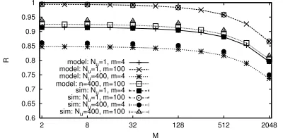
M model: Nu=1, m=4 model: Nu=1, m=100 model: Nu=400, m=4 model: n=400, m=100 sim: Nu=1, m=4 sim: Nu=1, m=100 sim: Nu=400, m=4 sim: Nu=400, m=100
Figure 5. The power save time ratio computed forTln=Tsub/3.
E[σ]. Figure 5 illustrates the power save time ratio R. Model’s and simulation’s results are very close in all cases, and confidence intervals are very small, so we omitted them in the figure. The results are sensitive to mandNu, while the effect ofM is almost negligible for short timeouts.
In conclusion, simulations suggest that we can safely use the model to estimate the system performance and evaluate its potentialities for power save with good accuracy.
B. Model-based parameter optimization
Here we want to compute the optimal values of m and M that yield the highest gain while keeping low the access delay and the download time. We consider the eNB cost only, but the results can be easily extended to the UE.
Reasonably, the cost for transmitting a data packet is larger than the cost for transmitting a control packet, which usually takes less bandwidth. Both transmitting and signal-ing costs are much higher than the cost to stay on, which, in turn, is at least one order of magnitude greater than the cost to stay in power save mode. As an example, we use
0 10 20 30 40 50 60 70 80 90 100
2 8
32 128
512 2048
0.02 0.04 0.06 0.08 0.1 0.12 0.14 0.16
E[D] [s]
m
M E[D] [s]
Figure 6. Access delay (independent on the number of users).
0 5 10 15 20 25 30 35 40
2 8
32
128 512
2048 8192
32768 0
0.1 0.2 0.3 0.4 0.5 0.6 0.7
GBS
Nu=1
Nu=10
Nu=100
m M
GBS
Figure 7. Relevant power save gain can be obtained with small timeouts, even for power save intervals lasting few subframes.
the following values: ctx = 100, csg = 50, con = 10, and cps = 1. Additionally, as suggested by experimental measurements [15], we consider a base station cost one order of magnitude higher than the transmission cost:cf = 1000. We assume that control packets have a durationTln= Tsub3 , e.g., the UE has to listen to the control channel only during the first of the three slots composing an HSPA subframe.
The access delay experienced in the network is reported in Figure 6.E[D]is sensitive tom, especially with low timeout values. However, reasonable values of m, e.g., below 20, yield access delay times not higher than 40 ms.
With the chosen cost parameters, the functionγ′(m)—not
0 0.1 0.2 0.3 0.4 0.5 0.6 0.7 0.8
0 50 100 150 200 250 300 350 400 450 500 GBS
Nu M=2, m=4
M=2, m=100
M=512, m=4 M=512, m=100
Figure 8. A large gain can be obtained over a wide spectrum of number of users as soon asmgrows to few tens.
0 0.2 0.4 0.6 0.8 1
400 350 300 100 10 1
Optimal eNB gain
Nu (256,9) (2,254) (2,58) (2,160)
(256,9) (2,254) (2,58) (2,160)
(256,9)
(2,254) (2,58) (2,160)
(256,9)
(2,254) (2,58) (2,160)
(256,9)
(2,114) (2,58) (2,160)
(-,-) (-,-) (2,58) (2,160) Dx=0.01 s, Wx=1.0 s
Dx=0.50 s, Wx=1.0 s Dx=0.10 s, Wx=5.0 s Dx=0.30 s, Wx=5.0 s
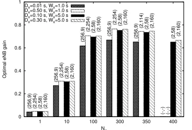
Figure 9. Relative gain for different number of users, optimized over bounded download time and access delay.
is labeled with the pair (M, m) which corresponds to the optimum. The figure shows that the gain can exceed 70% while keeping the access delay bounded to less than half second, and the total web page download time below one second. However, with 400 users, the minimum download time grows above one second and the system cannot be optimized unlessWxwas raised to a few seconds. Note also that the optimization with very small values of the access delay can only be obtained by setting a long timeout and short power save intervals (e.g.,M = 256andm= 9 with 100 users yields a∼60%gain with no more than 10 ms of access delay). With higher access delay bounds, e.g., as high as 100 ms, the optimal timeout is the shortest possible, i.e., M = 2. Almost in all cases, the optimization suggests to use very large values form. However, observing Figure 7, it is clear that near-optimal gain can be obtained with values ofmas low as 20.
VII. CONCLUSIONS
The paper shows how to model and simulate aG/G/1P S system representing the download transmission queues of cellular users adopting the continuous connectivity model. The model, which has been validated through simulation, is based on two basic assumptions:(i)users can receive traffic according to the DRX paradigm, and(ii)the user generated traffic is a realistic sequence of web page requests. We model the per-user activity and evaluate the service share that the base station processor can grant to each user. Furthermore, we propose a cost model and show how to optimize the power save parameters to minimize the cost under bounded
access delay and page download time. Remarkably, we show that up to 70% or more of the downlink transmission cost can be saved while preserving the quality of packet flows.
REFERENCES
[1] Nujira Ltd., “State of the art RF power technology
for defense systems,” white paper, Feb. 2009,
http://www.nujira.com/ uploads/whitepapers/State of the Art RF Power Technology for Defence Systems EU.pdf.
[2] S. Yang and Y. Lin, “Modeling UMTS discontinuous recep-tion mechanism,” IEEE Transactions on Wireless Communi-cations, vol. 4, no. 1, pp. 312–319, Jan. 2005.
[3] K. Han and S. Choi, “Performance analysis of sleep mode operation in IEEE 802.16e mobile broadband wireless access systems,” in Proc. of IEEE VTC 2006-Spring, vol. 3, Mel-bourne, Australia, May 2006, pp. 1141–1145.
[4] J. Seo, S. Lee, N. Park, H. Lee, and C. Cho, “Performance analysis of sleep mode operation in IEEE 802.16e,” inProc. of IEEE VTC 2004-Fall, vol. 2, Los Angeles, California, USA, Sep. 2004, pp. 1169–1173.
[5] S. Alouf, E. Altman, and A.P. Azad, “M/G/1 queue with repeated inhomogeneous vacations applied to IEEE 802.16e power saving,” inProc. of ACM Sigmetrics, Annapolis, Mary-land, Jun. 2008.
[6] Y. Xiao, “Performance analysis of an energy saving mecha-nism in the IEEE 802.16e wireless MAN,” inProc. of IEEE CCNC, vol. 1, Jan. 2006, pp. 406–410.
[7] J. Almhana, Z. Liu, C. Li, and R. McGorman, “Traffic esti-mation and power saving mechanism optimization of IEEE 802.16e networks,” inProc. of IEEE ICC 2008, vol. 19-23, Beijin, China, May 2008, pp. 322–326.
[8] H. Choi and J. Limb, “A behavioral model of web traffic,” in
ICNP’99, Washington, DC, USA, Oct. 1999.
[9] 3GPP TS 25.214, “Physical layer procedures (FDD), rel. 8.”
[10] L. Zhou, H. Xu, H. Tian, Y. Gao, L. Du, and L. Chen, “Perfor-mance analysis of power saving mechanism with adjustable DRX cycles in 3GPP LTE,” inIEEE VTC 2008-Fall, Calgary, Alberta, Cananda, Sep. 2008, pp. 1–5.
[11] C. Bontu and E. Illidge, “DRX mechanism for power saving in LTE,”IEEE Communications Magazine, vol. 47, no. 6, pp. 48–55, Jun. 2009.
[12] T. Kolding, J. Wigard, and L. Dalsgaard, “Balancing power saving and single user experience with discontinuous recep-tion in LTE,” inProc. of IEEE ISWCS, 2008, pp. 713–717.
[13] E. Dahlman, S. Parkvall, J. Skold, and P. Beming, 3G
Evolution: HSPA and LTE for Mobile Broadband, Second ed. Oxford, UK: Academic Press, 2008.
[14] 3GPP2 C.R1002-B v1.0, “CDMA2000 evaluation methodol-ogy - Revision B,” Dec. 2009.
![Figure 2.System cycle with web traffic as defined in [14].](https://thumb-us.123doks.com/thumbv2/123dok_us/1118462.1613430/3.612.318.565.75.174/figure-cycle-web-trafc-dened.webp)