Size distortion of bootstrap tests: application to a unit root test

GREQAM

Groupement de Recherche en Economie

Quantitative d'Aix-Marseille - UMR-CNRS 6579 Ecole des Hautes Etudes en Sciences Sociales

Universités d'Aix-Marseille II et III

Document de Travail

n°2009-40

SIZE DISTORTION OF BOOTSTRAP TESTS:

APPLICATION TO A UNIT ROOT TEST

Russell DAVIDSON

August 2009

Size Distortion of Bootstrap Tests

Application to a Unit Root Test

by

Russell Davidson

Department of Economics and CIREQ McGill University

Montr´eal, Qu´ebec, Canada H3A 2T7

GREQAM

Centre de la Vieille Charit´e 2 Rue de la Charit´e

13236 Marseille cedex 02, France

russell.davidson@mcgill.ca

Abstract

Testing for a unit root in a series obtained by summing a stationary MA(1) process with a parameter close to -1 leads to serious size distortions under the null, on account of the near cancellation of the unit root by the MA component in the driving stationary series. The situation is analysed from the point of view of bootstrap testing, and an exact quantitative account is given of the error in rejection probability of a bootstrap test. A particular method of estimating the MA parameter is recommended, as it leads to very little distortion even when the MA parameter is close to -1. A new bootstrap procedure with still better properties is proposed. While more computationally demanding than the usual bootstrap, it is much less so than the double bootstrap.

Keywords: Unit root test, bootstrap, MA(1), size distortion JEL codes: C10, C12, C22

This research was supported by the Canada Research Chair program (Chair in Economics, McGill University), and by grants from the Social Sciences and Humanities Research Council of Canada and the Fonds Qu´eb´ecois de Recherche sur la Soci´et´e et la Culture. A first version of the paper was presented at the 2nd Annual Granger Centre Conference, on Bootstrap and Numerical Methods in Time Series. A second version was presented at the 4th London and Oxbridge Time Series Workshop, and at the Econometrics workshop held at Rimini in July 2009. I thank participants of all these conferences for useful comments.

August 2009

1. Introduction

There are well-known difficulties in testing for a unit root in a series obtained by summing a stationary series that is a moving average process with a parameterθ close to -1. Unless special precautions are taken, size distortions under the null lead to gross over-rejection of the null hypothesis of a unit root, on account of the near cancellation of the unit root by the MA component in the driving stationary series. We may cite Schwert (1989) and Perron and Ng (1996)in this regard. It is natural to ask if the bootstrap can alleviate the problem. Since the null hypothesis is actually false when θ=−1, we cannot expect much power when θ is close to -1, but we can hope to reduce size distortion.

Sieve bootstraps of one sort or another have been proposed for unit root testing when one wishes to be quite agnostic as to the nature of the driving process. One of the first papers to propose a sieve bootstrap is B¨uhlmann (1997). The idea was further developed in B¨uhlmann(1998), Choi and Hall(2000), and Park (2002). In Park (2003), it was shown that under certain conditions a sieve bootstrap test benefits from asymptotic refinements. The sieve in question is an AR sieve, whereby one seeks to model the stationary driving series by a finite-order AR process, the chosen order being data driven. Sieves based on a set of finite-order MA or ARMA processes are considered in Richard (2007b), and many of Park’s results are shown to carry over to these sieve bootstraps. In particular, as might be expected, the MA sieve has better properties than the more usual AR sieve when the driving process is actually MA(1).

The purpose of this paper is to study the determinants of size distortion of bootstrap tests, and to look for ways to minimise it. Therefore, the problem considered in this paper is very specific, and as simple as possible.

• The unit root test on which the bootstrap tests are based is the augmented Dickey-Fuller test.

• It is supposed that it is known that the driving stationary process is MA(1), so that the only unknown quantity is the MA parameter.

• The bootstrap is a parametric bootstrap, for which it is assumed that the innovations of the MA(1) process are Gaussian.

Thus no sieve is used in the bootstrap procedure; the bootstrap samples are always drawn from an MA(1) process. The reason for concentrating on such a specific problem is that the bootstrap DGP is completely characterised by a single scalar parameter. This makes it possible to implement a number of procedures that are infeasible in more general contexts. I make no effort to use some of the testing procedures that minimise the size distortion, because the size distortion is the main focus of the analysis. In addition, no mention is made in the paper of asymptotic theory or asymptotic refinements, other than to mention that the asymptotic validity of bootstrap tests of the sort considered here has been established by Park (2003).

The fact that the null hypothesis is essentially one-dimensional, parametrised by the MA parameter, means that the parametric bootstrap can be analysed particularly sim-ply. Because the bootstrap data-generating process (DGP) is completely determined by

one single parameter, it is possible to implement at small computational cost a theoretical formula for the bootstrap discrepancy, that is, the difference between the true rejection probability of a bootstrap test and the nominal significance level of the test. This makes it possible to estimate the bootstrap discrepancy much more cheaply than usual. Any procedure that gives an estimate of the rejection probability of a bootstrap test allows one to compute a corrected P value. This is just the estimated rejection probability for a bootstrap test at nominal level equal to the uncorrected bootstrap P value, that is, the estimated probability mass in the distribution of the bootstrapP value in the region more extreme than the realised P value.

Although it is straightforward to estimate the parameters of an AR(p) process by a linear regression, estimating the parameter(s) of an MA or ARMA process is much less simple. In Galbraith and Zinde-Walsh (1994) and (1997), estimators are proposed that are easy to compute, as they are based on running the sort of linear regression used for estimation of AR parameters. However, I show that their estimators are too inefficient for them to be used effectively in the bootstrap context when the MA parameter is close to -1. Although the maximum likelihood estimator is easy enough to program, I have found that computation time is much longer than for the Galbraith and Zinde-Walsh (GZW) techniques. Further, the MLE has the odd property that its distribution sometimes has an atom with positive probability located at the point where the parameter is exactly equal to -1. A bootstrap DGP with parameter equal to -1 violates a basic principle of bootstrapping, since such a DGP does not have a unit root, whereas the null hypothesis of a unit root test is that one does exist. Here, I propose estimators based on nonlinear least squares (NLS) that are faster to compute than the MLE, although slower than the GZW estimators. They seem almost as efficient as maximum likelihood, and have no atom at -1. It is shown that they work very well for bootstrapping.

In Section 2, the NLS estimators of the parameters of MA and ARMA processes are described, and given in specific detail for MA(1). In Section 3, the distribution of the NLS estimator for an MA(1) process is compared with those of the MLE and the GZW estimators in a set of simulation experiments. It is found that the GZW estimators are seriously biased and have large variance when the true MA parameter is close to -1. The NLS and ML estimators, on the other hand, are much less biased and dispersed, and resemble each other quite closely, except that the NLS estimator has no atom at -1. Then, in Section 4, the bootstrap discrepancy is studied theoretically, and shown to depend on the joint bivariate distribution of two random variables. In Section 5, simulation-based methods for estimating the bootstrap discrepancy, and approximations to the discrepancy, are studied and compared in another set of simulation experiments. Section 6 studies three possible corrected bootstrap tests: the double bootstrap of Beran (1988), the fast double bootstrap of Davidson and MacKinnon (2007), and a new bootstrap, dubbed the discrepancy-corrected bootstrap, that is a good deal less computationally intensive than the double bootstrap, although more so than the fast double bootstrap. It is seen to be at least as good as the other two corrected bootstraps. InSection 7, a possible way to correct the fast double bootstrap is discussed. Simulation experiments that investigate the power of the bootstrap test are presented in Section 8, and some concluding remarks are offered in Section 9.

2. Estimating ARMA models by Nonlinear Least Squares

Suppose that the times series ut is generated by an ARMA(p, q) process, that we write as (1 +ρ(L))ut = (1 +θ(L))εt, (1) where L is the lag operator, ρ and θ are polynomials of degree p and q respectively:

ρ(z) = p X i=1 ρizi and θ(z) = q X j=1 θjzj.

Note that neither polynomial has a constant term. We wish to estimate the coefficients ρi, i= 1, . . . , p, and θj, j = 1, . . . , q, from an observed sample ut, t = 1, . . . , n, under the assumption that the series εt is white noise, with variance σ2.

In a model to be estimated by least squares, the dependent variable, here ut, is expressed as the sum of a regression function, which in this pure time-series case is a function of lags of ut, and a white-noise disturbance. The disturbance is εt, and so we solve for it in (1) to get

ε= (1 +θ(L))−1(1 +ρ(L))u.

Here, we may omit the subscriptt, and interpret uandεas the whole series. Since ρandθ have no constant term, the current value, ut, appears on the right-hand side only once, with coefficient unity. Thus we have

ε=u+¡(1 +θ(L))−1(1 +ρ(L))−1¢u

=u+ (1 +θ(L))−1¡1 +ρ(L)−(1 +θ(L))¢u. The nonlinear regression we use for estimation is then

u= (1 +θ(L))−1_{(θ(L)−ρ(L))u+ε. (2)} Write R(L) = (1 +θ(L))−1_{(θ(L)−ρ(L)). The regression function R(L)u is a nonlinear} function of the ARMA parameters, the ρi and the θj.

A good way to compute series like R(L)u or its derivatives is to make use of the operation of convolution. For two series a and b, the convolution series cis defined by

ct = t X s=0

asbt−s, t= 0,1,2, . . . . (3)

The first observation is indexed by 0, because the definition is messier if the first index is 1 rather than 0. Convolution is symmetric in a and b and is linear with respect to each argument. In fact, the ct are just the coefficients of the polynomialc(z) given by the product a(z)b(z), witha(z) =P_tatzt_{, and similarly for b(z) and c(z).}

Define the convolution operator C in the obvious way: C(a, b) =c, wherecis the series with ct given by (3). Although the coefficients of the inverse of a polynomial can be computed using the binomial theorem, it is easier to define an inverse convolution function C−1 _such that

a= C−1(c, b) iff c= C(a, b).

Inverse convolution isnot symmetric with respect to its arguments. It is linear with respect to its first argument, but not the second. It is easy to compute an inverse convolution recursively. If the relation is (3), then, if b0 = 1 as is always the case here, we see that

a0 =c0 and at =ct−

t−1 X s=0

asbt−s.

Note that C(a, e0) = a and C−1_{(a, e0) = a where (e0)t = δt0. This corresponds to the} fact that the polynomial 1 is the multiplicative identity in the algebra of polynomials. In addition, if the seriesej is defined so as to have elementtequal to δtj, then C(a, ej) = Lj_a. Leta be the series the first element (element 0) of which is 1, elementiof which is the AR parameter ρi, for i= 1, . . . , p, and elements at for t > p are zero. Define b similarly with the MA parameters. Then the series r containing the coefficients of R(L) is given by

r= C−1(b−a, b),

and the series R(L)u is just C(u, r). The derivatives of R(L)u with respect to the ρi and the θj are also easy to calculate.

MA(1)

It is useful to specialise the above results for the case of an MA(1) process. The series a is then e0, and b is e0 +θe1, where we write θ instead of θ1, since there are no other parameters. Then R(L) =θ(1 +θL)−1_{L, and the coefficients of the polynomial R are the} elements of the series r = R(L)e0 = θC−1(Le0, b). Consequently, C(u, r) = θC−1(Lu, b). The only derivative of interest is with respect to θ; it is C−1¡_{L(u−C(u, r)), b}¢_.

The regression (2), which we write as u = R(L)u +ε, is not in fact accurate for a fi-nite sample, because the convolution operation implicitly sets the elements with negative indices of all series equal to 0. For the first element, the regression says therefore that u0 = ε0, whereas what should be true is rather that u0 = ε0 +θε−1. Thus the rela-tion u−θε−1e0 = (1 +θL)ε is true for all its elements if the lag of ε0 is treated as zero.

We write φ = θε−1, and treat φ as an unknown parameter. The regression model (2) is replaced by

u=φe0+θ(1 +θL)−1L(u−φe0) +ε. (4) Although it is perfectly possible to estimate (4) by nonlinear least squares, with two parameters, θ and φ, it is faster to perform two nonlinear regressions, each with only one parameter θ. When there is only one parameter, the least-squares problem can be solved as a one-dimensional minimisation. The first stage sets φ = 0 in order to get a

preliminary estimate of θ; then, for the second stage, φ is estimated from the first-stage result, and the result used as a constant in the second stage. The first-order condition for φ in the regression (4) is

¡

(1−R(L)e0¢>¡(1−R(L)¢(u−φe0)¢= 0.

Recalling that R(L)e0 =r and writinge0−r=s, we can write this condition as s>¡(1−R(L))u−φs¢= 0 whence φ= s

>_(1−R(L))u

s>_s .

In order to compute the estimate ofφfrom the first stage, the seriessis set up withs0 = 1, st =−rt for t > 0, and we note that (1−R(L))u is just the vector of residuals from the first stage regression.

3. Comparison of Estimators for MA(1)

Asymptotic efficiency in the estimation of the parameterθ of an MA(1) process is achieved by Gaussian maximum likelihood (ML) if the disturbances are Gaussian. But we saw that the MLE has an atom at -1 if the true θ is close to -1, and so it is of interest to see how much efficiency is lost by using other methods that do not have this feature.

The loglikelihood function for the MA(1) model is

`(θ, σ2) =−−n₂log 2πσ2−−1₂log detΣ(θ)− 1

2σ2u

>_Σ−1_{(θ)u, (5)}

whereσ2 _{= Var(εt) and Σ(θ) is an n×n Toeplitz matrix with all diagonal elements equal} to 1 +θ2 _{and all elements of the diagonals immediately below and above the principal} diagonal equal to θ. The notationu is just vector notation for the series u.

Concentrating with respect to σ2 _gives ˆ

σ2(θ) =−_n1u>Σ−1(θ)u. Thus the concentrated loglikelihood is

n

−₂(logn−log 2π−1)−−n₂ logu>Σ−1(θ)u−−1₂log detΣ(θ). (6) This expression can be maximised with respect to θ by minimising

`(θ)≡nlogu>Σ−1(θ)u+ log detΣ(θ), (7) and this can be achieved by use of any suitable one-dimensional minimisation algorithm, including Newton’s method.

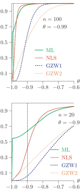
−1.0 −0.9 −0.8 −0.7 −0.6 0.1 0.3 0.5 0.7 0.9 ... ... ... ... ... ... ... ... ... ... ... ... ... ... ... ... _ML ... ... ... ... ... ... ... ... ... ... ... ... ... ... ... ... ... ... ... ... ... ... ... _NLS ... ... ... ... ... ... ... ... ... ... ... ... ... ... ... ... ... _GZW1 ... ... ... ... ... ... ... ... ... ... ... ... ... ... ... ... .. ... _GZW2 ... ... ... ... ... ... ... ... ... ... ... ... ... ... ... ... ... ... ... ... ... ... ... ... ... ... ... ... ... ... ... ... ... ... ... ... ... ... ... ... ... ... ... ... ... ... ... ... ... ... ... n= 100 θ =−0.9 θ −1.0 −0.9 −0.8 −0.7 −0.6 0.1 0.3 0.5 0.7 0.9 ... ... ... ... ... ... ... ... ... ... ... ... ... ... ... ... ... ... ... ... ... ... ... ... _ML ... ... ... ... ... ... ... ... ... ... ... ... ... ... ... ... ... ... ... ... ... ... ... ... ... ... ... ... ... ... ... _NLS ... ... ... ... ... ... ... ... ... ... ... ... ... ... ... ... _GZW1 ... ... ... ... ... ... ... ... ... ... ... ... ... ... ... ... ... ... _GZW2 ... ... ... ... ... ... ... ... ... ... ... ... ... ... ... ... ... ... ... ... ... ... ... ... ... ... ... ... ... ... ... ... ... ... ... ... ... ... ... ... ... ... ... ... ... ... ... ... ... ... ... n= 100 θ =−0.99 θ −0.2 −0.1 0.0 0.1 0.2 0.3 0.1 0.3 0.5 0.7 0.9 ... ... ... ... ... ... ... ... ... ... ... ... ... ... _ML ... ... ... ... ... ... ... ... ... ... ... ... ... ... ... ... ... ... ... ... ... ... ... _NLS ... ... ... ... ... ... ... ... ... ... ... ... ... ... ... ... ... _GZW1 ... ... ... ... ... ... ... ... ... ... ... ... ... ... ... ... _GZW2 n= 100 θ= 0 θ −1.0 −0.9 −0.8 −0.7 −0.6 0.1 0.3 0.5 0.7 0.9 ... ... ... ... ... ... ... ... ... ... ... ... ... ... ... ... ... ... ... ... ... ... _ML ... ... ... ... ... ... ... ... ... ... ... ... ... ... ... ... ... ... ... ... ... ... ... _NLS ... ... ... ... ... ... ... ... ... ... ... ... ... ... _GZW1 ... ... ... ... ... ... ... ... ... ... ... ... ... _GZW2 ... ... ... ... ... ... ... ... ... ... ... ... ... ... ... ... ... ... ... ... ... ... ... ... ... ... ... ... ... ... ... ... ... ... ... ... ... ... ... ... ... ... ... ... ... ... ... ... ... ... ... n= 20 θ =−0.9 θ Figure 1: Comparison of MA(1) estimators

Other methods for estimating MA models have been proposed by Galbraith and Zinde-Walsh(1994)and for ARMA models by the same authors(1997). Their methods are based on estimating the following AR(k) model by ordinary least squares:

ut = k X i=1

aiut−i + residual, t=k+ 1, . . . , n. (8) For an ARMA(p, q) model, k is chosen considerably greater than p+q. The estimators are consistent as k → ∞ while k/n → 0, but are not asymptotically efficient. They are however simple and fast to compute, as they involve no iterative procedure.

Let the OLS estimates of the parameters ai in (8) be denoted as ˆai. For the MA(1) model ut = εt +θεt−1, the simplest estimator of θ is just ˆa1. Another estimator, that can be

traced back to Durbin (1959), is the parameter estimate from the OLS regression of the vector [ˆa1. . .aˆk]>, on the vector [1 −aˆ1. . .−ˆak−1]>.

Any of the estimation methods so far discussed can give an estimate of θ outside the interval [−1,1]. But the processes with parameters θ and 1/θ are observationally equiv-alent. Thus whenever an estimate outside [−1,1] is obtained, it is simply replaced by its reciprocal. In Figure 1 are shown estimated cumulative distribution functions (CDFs) of four estimators, (Gaussian) maximum likelihood (ML), nonlinear least-squares using the two-stage procedure based on (4), with ρ(z) = 0, θ(z) =θz (NLS), Galbraith and Zinde-Walsh’s first estimator ˆa1 (GZW1), and their second estimator (GZW2). In all but the bottom right panel of the figure the sample size is n = 100. The distributions are shown for values ofθ of -0.9, -0.99, and 0. The length of the GZW preliminary autoregression (8) is k = 20. In the bottom right panel, n= 20, θ =−0.9, and k = 6. It is well known that the greatest challenge for estimators of the MA(1) parameter arises when θ is close to -1. The overall picture is clear enough. Both ML and NLS outperform the GZW estimators except when θ = 0, or, more generally, whenθ is distant from -1. GZW1 has much greater variance than the other estimators, and GZW2 is heavily biased to the right. For n= 20, the concentration of ML estimates close to -1 is seen; the other estimators do not exhibit this feature, which is much less visible for ML itself for the larger sample size. ML and NLS are almost unbiased for n= 100, and do not greatly differ. Experiments with other values of θ show that the four estimators have similar distributions when n is large enough and θ is greater than around -0.5 The inescapable conclusion is that using the GZW estimator in order to define a bootstrap DGP will give rise to serious size distortion.

4. The Bootstrap Discrepancy

Suppose that a test statistic τ is designed to test a particular null hypothesis. The set of all DGPs that satisfy that hypothesis is denoted as M0; this set constitutes what we may call the null model. A bootstrap test based on the statisticτ approximates the distribution of τ under a DGP µ ∈ M0 by its distribution under a bootstrap DGP that also belongs to M0 and can be thought of as an estimate of the true DGP µ.

We define the bootstrap discrepancy as the difference, as a function of the true DGP and the nominal level, between the actual rejection probability of the bootstrap test and the nominal level. In order to study it, we suppose, without loss of generality, that the test statistic is already in approximate P value form, so that the rejection region is to the left of a critical value.

The rejection probability functionRdepends both on the nominal levelα and the DGPµ. It is defined as

R(α, µ)≡Prµ(τ < α). (9)

We assume that, for all µ∈ M0, the distribution of τ has support [0,1] and is absolutely continuous with respect to the uniform distribution on that interval. For givenµ, R(α, µ) is just the CDF of τ evaluated at α. The inverse of the rejection probability function is the critical value function Q, which is defined implicitly by the equation

Prµ¡τ < Q(α, µ)¢=α. (10)

It is clear from (10) that Q(α, µ) is the α-quantile of the distribution of τ under µ. In addition, the definitions (9) and (10) imply that

R¡Q(α, µ), µ¢=Q¡R(α, µ), µ¢ =α (11) for all α and µ.

In what follows, we ignore simulation randomness in the estimate of the distribution of τ under the bootstrap DGP, which we denote by µ∗_{. The bootstrap critical value for τ at}

levelαisQ(α, µ∗_{). Rejection by the bootstrap test is the eventτ < Q(α, µ}∗_{). Applying the}

increasing transformation R(·, µ∗_{) to both sides and using (11), we see that the bootstrap}

test rejects whenever

R(τ, µ∗_{)< R}¡_{Q(α, µ}∗_{), µ}∗¢_=α.

Thus the bootstrap P value is just R(τ, µ∗_{), which can therefore be interpreted as a}

bootstrap test statistic.

If instead we apply the increasing transformation R(·, µ) to the inequality τ < Q(α, µ∗_),

it follows that rejection by the bootstrap test can also be expressed as R(τ, µ) < R¡Q(α, µ∗_{), µ}¢_{. We define two random variables, one a deterministic function of τ, the}

other a deterministic function of µ∗_{, the other random element involved in the bootstrap}

test. The first variable is p≡R(τ, µ). It is distributed as U(0,1) under µ, because R(·, µ) is the CDF of τ under µ and because we have assumed that the distribution of τ is ab-solutely continuous on the unit interval for all µ ∈ M. The second random variable is q ≡R(Q(α, µ∗_{), µ)−α =R(Q(α, µ}∗_{), µ)−R(Q(α, µ), µ). Thus rejection by the bootstrap}

test is the eventp < α+q. Let the CDF ofq underµconditional on the random variablep be denoted as F(q | p). Then it is shown in Davidson and MacKinnon (2006) that the bootstrap discrepancy can be expressed as

Z _1−α

−α

xdF(x |α+x). (12)

The random variableq+α is the probability that a statistic generated by the DGPµis less than the α-quantile of the bootstrap distribution, conditional on that distribution. The expectation ofq can thus be interpreted as the bias in rejection probability when the latter is estimated by the bootstrap. The actual bootstrap discrepancy, which is a nonrandom quantity, is the expectation of q conditional on being at the margin of rejection.

We study the critical value function of the test statistic most frequently used to test the null hypothesis of a unit root, namely the augmented Dickey-Fuller (ADF) test. The DGPs used to generate the data of the simulation experiment take the form

ut =εt +θεt−1, yt =y0+

t X s=1

ut, (13)

−1.0 −0.8 −0.6 −0.4 −0.2 0.0 −7.0 −6.0 −5.0 −4.0 −3.0 −2.0 .... .... .... .... .... .... .... .... .... ... .... .... .... .... .... .... .... .... .... ... .... .... .... .... .... .... .... .... .... ... .... .... .... .... .... .... .... .... .... ... .... .... .... .... .... .... .... .... ... .... .... .... .... .... .... .... .... .... ... .... .... .... .... .... .... .... .... .... ... .... .... .... .... .... .... .... .... .... ... .... .... .... .... .... .... .... .... .... ... .... .... .... .... .... .... .... .... .... ... ... ... ... ... ... ... ... ... ... ... ... ... ... ... ... ... ... ... ... ... ... ... ... ... ... ... ... ... ... ... ... ... ... ... ... ... ... ... ... ... ... ... ... ... ... ... ... ... .... .... ... 0.01 quantile .... .... .... .... .... .... .... .... .... ... .... .... .... .... .... .... .... .... .... ... .... .... .... .... .... .... .... .... .... ... .... .... .... .... .... .... .... .... .... ... .... .... .... .... .... .... .... .... ... .... .... .... .... .... .... .... .... .... ... .... .... .... .... .... .... .... .... .... ... .... .... .... .... .... .... .... .... .... ... .... .... .... .... .... .... .... .... ... .... .... .... .... .... .... .... .... .... ... ... ... ... ... ... ... ... ... ... ... ... ... ... ... ... ... ... ... ... ... ... ... ... ... ... ... ... ... ... ... ... ... ... ... ... ... ... ... ... ... ... ... ... ... ... ... ... ... ... ... ... ... ... 0.05 quantile .... .... .... .... .... .... .... .... .... ... .... .... .... .... .... .... .... .... .... ... .... .... .... .... .... .... .... .... .... ... .... .... .... .... .... .... .... .... .... ... .... .... .... .... .... .... .... .... ... .... .... .... .... .... .... .... .... .... ... .... .... .... .... .... .... .... .... .... ... .... .... .... .... .... .... .... .... .... ... .... .... .... .... .... .... .... .... ... .... .... .... .... .... .... .... .... .... ... .... .... .... .... .... .... .... .... ... ... ... ... ... ... ... ... ... ... ... ... ... ... ... ... ... ... ... ... ... ... ... ... ... ... ... ... ... ... ... ... ... ... ... ... ... ... ... ... ... ... ... ... ... ... ... 0.10 quantile θ q −1.0 −0.8 −0.6 −0.4 −0.2 0.0 −150.0 −130.0 −110.0 −90.0 −70.0 −50.0 −30.0 −10.0 .... .... .... .... .... .... .... .... .... ... .... .... .... .... .... .... .... .... .... ... .... .... .... .... .... .... .... .... .... ... .... .... .... .... .... .... .... .... .... ... .... .... .... .... .... .... .... .... .... ... .... .... .... .... .... .... .... .... .... ... .... ... .... .... .... .... .... .... .... ... ... ... ... ... ... ... ... ... ... ... ... ... ... ... ... ... ... ... ... ... ... ... ... ... ... ... ... ... ... ... ... ... ... ... ... ... ... ... ... ... ... ... ... ... ... ... ... ... ... ... ... ... ... ... ... ... ... ... ... ... ... ... ... ... ... ... ... ... ... ... ... 0.01 quantile .... .... .... .... .... .... .... .... .... ... .... .... .... .... .... .... .... .... .... ... .... .... .... .... .... .... .... .... .... ... .... .... .... .... .... .... .... .... .... ... .... .... .... .... .... .... .... .... .... ... .... .... .... .... .... .... .... .... .... ... .... .... .... .... .... .... .... .... .... ... .... .... .... .... .... .... .... .... .... ... ... ... .... ... ... ... ... ... ... ... ... ... ... ... ... ... ... ... ... ... ... ... ... ... ... ... ... ... ... ... ... ... ... ... ... ... ... ... ... ... ... ... ... ... ... ... ... ... ... ... ... ... ... ... ... ... ... ... ... ... ... ... ... ... ... . ... 0.05 quantile .... .... .... .... .... .... .... .... .... ... .... .... .... .... .... .... .... .... .... ... .... .... .... .... .... .... .... .... .... ... .... .... .... .... .... .... .... .... .... ... .... .... .... .... .... .... .... .... ... .... .... .... .... .... .... .... .... .... ... .... .... .... .... .... .... .... .... .... ... .... .... .... .... .... .... .... .... .... ... .... .... .... .... .... .... .... .... .... ... ... ... .... ... ... ... ... ... ... ... ... ... ... ... ... ... ... ... ... ... ... ... ... ... ... ... ... ... ... ... ... ... ... ... ... ... ... ... ... ... ... ... ... ... ... ... ... ... ... ... ... ... ... ... ... ... ... ... ... ... ... 0.10 quantile θ q τc n= 100, p= 3 zc −1.0 −0.8 −0.6 −0.4 −0.2 0.0 −4.0 −3.0 −2.0 .... .... .... .... .... .... .... .... .... ... .... .... .... .... .... .... .... .... .... ... .... .... .... .... .... .... .... .... .... ... .... .... .... .... .... .... .... .... .... ... .... .... .... .... .... .... .... .... ... .... .... .... .... .... .... .... .... .... ... .... .... .... .... .... .... .... .... .... ... .... .... .... .... .... .... .... .... .... ... .... .... .... .... .... .... .... .... ... .... .... .... .... .... .... .... .... .... ... .... .... .... .... .... .... .... .... .... ... .... .... .... .... .... .... .... .... .... ... .... .... .... .... .... .... .... .... ... .... .... .... .... .... .... .... .... .... ... .... .... .... .... .... .... .... .... .... ... ... ... .... ... ... ... ... ... ... ... ... ... ... ... ... ... ... ... ... ... ... ... ... ... .... . ... 0.01 quantile .... .... .... .... .... .... .... .... .... ... .... .... .... .... .... .... .... .... .... ... .... .... .... .... .... .... .... .... .... ... .... .... .... .... .... .... .... .... .... ... .... .... .... .... .... .... .... .... ... .... .... .... .... .... .... .... .... .... ... .... .... .... .... .... .... .... .... .... ... .... .... .... .... .... .... .... .... .... ... .... .... .... .... .... .... .... .... ... .... .... .... .... .... .... .... .... .... ... .... .... .... .... .... .... .... .... .... ... .... .... .... .... .... .... .... .... .... ... .... .... .... .... .... .... .... .... ... .... .... .... .... .... .... .... .... .... ... .... .... .... .... .... .... .... .... .... ... ... ... ... ... ... ... ... ... ... ... ... ... ... ... ... ... ... ... ... ... ... ... ... ... ... ... ... 0.05 quantile .... .... .... .... .... .... .... .... .... ... .... .... .... .... .... .... .... .... .... ... .... .... .... .... .... .... .... .... .... ... .... .... .... .... .... .... .... .... .... ... .... .... .... .... .... .... .... .... ... .... .... .... .... .... .... .... .... .... ... .... .... .... .... .... .... .... .... .... ... .... .... .... .... .... .... .... .... .... ... .... .... .... .... .... .... .... .... ... .... .... .... .... .... .... .... .... .... ... .... .... .... .... .... .... .... .... .... ... .... .... .... .... .... .... .... .... .... ... .... .... .... .... .... .... .... .... ... .... .... .... .... .... .... .... .... .... ... .... .... .... .... .... .... .... .... .... ... ... ... ... ... ... ... ... ... ... ... ... ... ... ... ... ... ... ... ... ... ... ... ... ... ... ... ... 0.10 quantile θ q −1.0 −0.8 −0.6 −0.4 −0.2 0.0 −260.0 −220.0 −180.0 −140.0 −100.0 −60.0 −20.0 _.... .... .... .... .... .... .... .... .... ... .... .... .... .... .... .... .... .... .... ... .... .... .... .... .... .... .... .... .... ... .... .... .... .... .... .... .... .... .... ... .... .... .... .... .... .... .... .... .... ... .... .... .... .... .... .... .... .... .... ... .... .... .... .... .... .... .... .... .... ... .... .... .... .... .... .... .... .... .... ... .... ... .... .... .... .... ... .... .... ... ... ... ... ... ... ... ... ... ... ... ... ... ... ... ... ... ... ... ... ... ... ... ... ... ... ... ... ... ... ... ... ... ... ... ... ... ... ... ... ... ... ... ... ... ... ... ... ... ... ... ... ... ... ... ... ... ... ... ... ... ... ... ... ... ... ... 0.01 quantile .... .... .... .... .... .... .... .... .... ... .... .... .... .... .... .... .... .... .... ... .... .... .... .... .... .... .... .... .... ... .... .... .... .... .... .... .... .... .... ... .... .... .... .... .... .... .... .... ... .... .... .... .... .... .... .... .... .... ... .... .... .... .... .... .... .... .... .... ... .... .... .... .... .... .... .... .... .... ... .... .... .... .... .... .... .... .... .... ... .... .... .... .... .... .... .... .... .... ... .... .... .... .... .... .... .... .... .... ... ... ... ... ... ... ... ... ... ... ... ... ... ... ... ... ... ... ... ... ... ... ... ... ... ... ... ... ... ... ... ... ... ... ... ... ... ... ... ... ... ... ... ... ... ... ... ... ... ... ... ... ... ... ... 0.05 quantile .... .... .... .... .... .... .... .... .... ... .... .... .... .... .... .... .... .... .... ... .... .... .... .... .... .... .... .... .... ... .... .... .... .... .... .... .... .... .... ... .... .... .... .... .... .... .... .... ... .... .... .... .... .... .... .... .... .... ... .... .... .... .... .... .... .... .... .... ... .... .... .... .... .... .... .... .... .... ... .... .... .... .... .... .... .... .... .... ... .... .... .... .... .... .... .... .... .... ... .... .... .... .... .... .... .... .... .... ... .... .... .... .... .... .... .... .... .... ... ... ... ... ... ... ... ... ... ... ... ... ... ... ... ... ... ... ... ... ... ... ... ... ... ... ... ... ... ... ... ... ... ... ... ... ... ... ... ... ... ... ... ... ... ... . _{... 0.10 quantile} θ q τc n= 100, p= 12 zc

Figure 2: Critical value functions

where the εt are IID N(0,1). The test statistics are computed using the ADF testing regression ∆yt =β0+β1yt−1+ p X i=1 γi∆yt−1 + residual. (14) When this regression is run by ordinary least squares, thezc statistic isnβ1; theˆ τc statistic is the conventional t statistic for the hypothesis that β1 = 0. Under the null hypothesis that the series yt has a unit root, these two statistics have well-known but nonstandard

asymptotic distributions.

The variance of the εt is set to 1 without loss of generality, since both statistics are scale invariant. In fact, both statistics are also numerically invariant to changes in the value of the starting valuey0, and so we can without loss of generality sety0 = 0 in our simulations. We vary the MA parameterθ from 0 to -0.8 by steps of 0.05, and from -0.8 to -0.99 by steps of 0.01. For each value we estimate the 0.01, 0.05, and 0.10 quantiles of the distribution of each statistic, using 99,999 replications. The same random numbers are used for each value of θ in order to achieve a smoother estimate of the critical value function, which is the quantile of the statistic as a function of θ.

Figure 2shows the 0.01, 0.05, and 0.1 quantiles for theτcandzc statistics. We could obtain the CVFs of the statistics by transforming them by the inverse of the nominal asymptotic CDFs of the statistics. In the upper panels, the sample size n= 100 and the number p of lags of ∆yt is 3. In the lower panels, the quantiles are graphed for n = 100 and p = 12. The choice of the statistic τc and of p = 12 gives the smallest variation of the CVF, and so, for the rest of this study, we examine the consequences of making this choice.

5. Estimating the Bootstrap Discrepancy

Brute force

The conventional way to estimate the bootstrap rejection probability (RP) for a given DGPµand sample size nby simulation is to generate a large number,M say, of samples of sizenusing the DGPµ. For each replication, a realizationτmof the statisticτ is computed from the simulated sample, along with a realization ˆµm of the bootstrap DGP. Then B bootstrap samples are generated using ˆµm, and bootstrap statistics τ∗

mj, j = 1, . . . , B are computed. The realized bootstrap P value for replication mis then

ˆ p∗_m(τm)≡ 1 B B X j=1 I(τ_mj∗ < τm), (15) where we assume that the rejection region is to the left. The estimate of the RP at nominal levelα is the proportion of the ˆp∗

m(τm) that are less thanα. The whole procedure requires the computation of M(B+ 1) statistics andM bootstrap DGPs. The bootstrap statistics τ∗

mj are realizations of a random variable that we denote as τ∗.

If one wishes to compare the RP of the bootstrap test with that of the underlying asymp-totic test, a simulation estimate of the latter can be obtained directly as the proportion of the τm less than the asymptotic α level critical value. Of course, estimation of the RP of the asymptotic test by itself requires the computation of only M statistics.

Denote by p∗

1 the ideal bootstrap P value, that is, the probability mass in the distribution of the bootstrap statistics in the region more extreme than the realisation ˆτ of the statistic computed from the real data. Let the probability space in which statistics and bootstrap DGPs are defined be (Ω,F, P). The statistic ˆτ can then be written as τ(ω, µ), where

ω ∈ Ω and µ is the true DGP. The bootstrap DGP can be expressed as µ(ω, µ), for the same realisationωas for ˆτ. In a simulation context, the probability space can be considered that of the random number generator. With real data, ω is just a way of representing all the random elements that gave rise to the data.

The bootstrap P value can be expressed as

p∗₁(ω, µ) = Prµ(τ∗ <τˆ) = Eµ¡I(τ∗ <τˆ)|ω¢,

where τ∗ _{is the bootstrap statistic. A realisation of τ}∗ _{is τ}¡_ω∗_{, µ(ω, µ)}¢_{, where ω}∗ _{∈ Ω is}

independent of ω. The P value is thus p∗

1(ω, µ) = Z

Ω

I¡τ(ω∗_{, µ(ω, µ))< τ(ω, µ)}¢_dP(ω∗_{). (16)}

Let R(x, µ) be the CDF of τ under µ. This means that R(x, µ) = Pr¡τ(ω, µ)< x¢=

Z Ω

I¡τ(ω, µ)< x¢dP(ω), and so, from (16),

p∗₁(ω, µ) =R¡τ(ω, µ), µ(ω, µ)¢. We denote the CDF of this random variable by R1(x, µ), so that

R1(x, µ) = Prµ(p∗₁(µ, ω)≤x) = Eµ ³

I¡R(τ(µ, ω), b(µ, ω))≤x¢´. (17)

The fast approximation

It is shown in Davidson and MacKinnon(2007)that, under certain conditions, it is possible to obtain a much less expensive approximate estimate of the bootstrap RP, as follows. As before, form= 1, . . . , M, the DGPµis used to draw realizations τm and ˆµm. In addition, ˆ

µmis used to draw asingle bootstrap statisticτ∗

m. Theτm∗ are therefore IID realizations of the variableτ∗_{. We estimate the RP as the proportion of the τm that are less than ˆQ}∗_(α),

the α quantile of the τ∗

m. This yields the following estimate of the RP of the bootstrap test: c RPA ≡ 1 M M X m=1 I¡τm<Qˆ∗(α)¢,

As a function of α, RPcA is an estimate of the CDF of the bootstrap P value.

The above estimate is approximate not only because it rests on the assumption of the full independence of τ and µ∗_{, but also because its limit as B → ∞ is not precisely the RP}

of the bootstrap test. Its limit differs from the RP by an amount of a smaller order of magnitude than the difference between the RP and the nominal level α. But it requires the computation of only 2M statistics andM bootstrap DGPs.

Conditional on the bootstrap DGPµ∗_{, the CDF ofτ}∗ _{evaluated atxisR(x, µ}∗_{). Therefore,}

if µ∗ _{is generated by the DGP µ, the unconditional CDF of τ}∗ _is

R∗(x, µ)≡Eµ¡R(x, µ∗)¢.

We denote the α quantile of the distribution of τ∗ _{under µ by Q}∗_{(α, µ). In the explicit}

notation used earlier, sinceτ∗ _=τ¡_ω∗_{, µ(ω, µ)}¢_{, we see that}

R∗(x, µ) = Z Ω Z Ω I ³ τ¡ω∗, µ(ω, µ)¢< x ´ dP(ω∗) dP(ω). (18)

Evaluating the analytic expression

The formula (12) cannot be implemented unless one knows the function F, the CDF of q conditional on p. This function can be estimated arbitrarily well by simulation if we can generate IID joint realisations of p and q. But that is made difficult by the fact that, for a given DGPµ, both p and q are defined in terms of the functionsR and Q, which are in general unknown. Estimating R andQ by simulation is also quite possible, for a givenµ. Butqis defined using the bootstrap DGPµ∗_{, and, since this is random, we cannot estimate}

Q(·, µ∗_{) for all possible realisations of µ}∗ _{in a single experiment.}

The case of the model with DGPs of the form (13) is much more tractable than most, however, since the bootstrap DGP is completely determined by a single parameter. It is therefore convenient to replace the notationµbyθ. Simulations of the sort used to obtain the data graphed inFigure 2 can be used for simulation-based estimates ofQ(α, θ) for any given α and θ. For a set of values of α and a set of values of θ, we can construct a table giving the values of Q(α, θ) for the chosen arguments. There are as many experiments as there are values ofθ, but, as for Figure 3, it is advisable to use the same random numbers for each experiment. Each experiment allows us to estimate all the quantiles Q(α, θ) for the relevant θ.

The most direct way to proceed after setting up the table is as follows. Choose a DGP by specifying the parameter θ, and choose a nominal level α. Use the chosen DGP to generate many joint realisations of the pair (τ,θ). Approximateˆ Q(α,θ) by interpolationˆ based on the values in the table for the chosen α and the set of θ values, obtaining the approximation ˜Q(α,θ). Then the rejection probability of the bootstrap test at levelˆ α is estimated by the proportion of realisations for which τ <Q(α,˜ θ).ˆ

Alternatively, an experiment that more closely mimics the theoretical discussion leading to (12) is as follows. Perform a set of experiments in which we obtain simulation-based estimates of R(Q(α, θ1), θ2) for the set of values chosen for α, and for any pair (θ1, θ2) of values in the set chosen for θ. Here we need only as many experiments as there are values ofθ, since, after fixing θ2, we generate a large number ofτ statistics using the DGP characterised byθ2, and then, for each value ofQ(α, θ1) in the set, estimateR(Q(α, θ1), θ2) as the proportion of the generated statistics less than Q(α, θ1).

Now suppose that a single realisation from the DGP characterised by a value of θ in the chosen set gives rise to an estimate ˆθ. For given α, we can then use the simulated values of R(Q(α, θ1), θ) in order to interpolate the value ofR(Q(α,θ), θ). As Figure 3 shows, theˆ quantiles vary quite smoothly as functions of θ, and so interpolation should work well. In the experiments to be described, cubic splines were used for this purpose.

If we now repeat the operation of the previous paragraph many times, we get a set of realisations of the random variable q by subtracting α from the simulated R(Q(α,θ), θ).ˆ But for each repetition, we also compute the value of the τ statistic, and keep the pair (τ, q). When all the repetitions have been completed, we sort the pairs in increasing order of τ. For each repetition, then, we estimate the random variable p by the index of the associated pair in the sorted set, divided by the number of repetitions. This is equivalent to using the set of generated τ values to estimate R(·, θ), and evaluating the result at the particular τ for each repetition. We end up with a set of IID joint realisations of p andq. At this point, our estimate of the RP of the bootstrap test at significance level α is just the proportion of the repetitions for which p < α+q, and the estimate of the bootstrap discrepancy is the estimated RP minus α. It is of interest to see how close two approxi-mations to the bootstrap discrepancy come to the estimate obtained in this way. Both of these can be readily computed using the set of joint realisations ofpandq. The first is the estimated expectation ofq, which is just the average of the realisedq, with no reference to the associated p. The second is an estimate of the expectation of q conditional on p=α, that is,

Z _1−α

−α

xdF(x|α),

rather than the exact expression (12). This conditional expectation can readily be esti-mated with a kernel estimator.

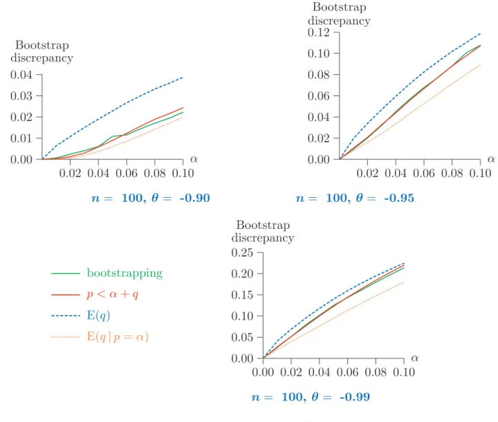
In Figure 3 are depicted plots of the bootstrap discrepancy as a function of the nominal level α for values between 0.01 and 0.10. The three panels show results for three different true DGPs, with θ = 0.90, 0.95, and 0.99, with sample size n= 100. The NLS procedure was used for the estimation ofθ. Three simulation-based estimates are given. The first two were computed using 99,999 repetitions of the experiment described above, the first the proportion of repetitions withp < α+q, the second the expectation ofq. The expectation conditional on p = α is so close to the first estimate that it would not be distinguishable from it in the graph. The last estimate was computed after 10,000 repetitions of a full-blown bootstrap test, with 399 bootstrap repetitions.

It can be seen that the unconditional expectation of q is not a very good estimate of the bootstrap discrepancy. In all cases, it overestimates the RP. Of the other two estimates, the one based on the realisations of pandq is probably superior from the theoretical point of view, since the one based on full-blown bootstrapping, besides being based on fewer repetitions, gives the bootstrap discrepancy for a test with 399bootstrap repetitions, while the other estimates the theoretical bootstrap discrepancy, corresponding to an infinite number of bootstrap repetitions. An interesting inversion of the sign of the bootstrap discrepancy can be seen, with a negative discrepancy for both θ = −0.90 and θ =−0.95,

0.02 0.04 0.06 0.08 0.10 −0.05 −0.04 −0.03 −0.02 −0.01 0.00 ..._... ..._... ..._... ..._... ..._... ..._... ..._... ..._... ..._... ..._... ..._... ..._... ..._... ..._... ..._... ..._... ..._... ... ... α Bootstrap discrepancy 0.02 0.04 0.06 0.08 0.10 −0.02 −0.01 0.00 0.01 ..._... ..._... ..._... ..._... ... ..._... ..._... ..._... ..._... ..._... ... ... α Bootstrap discrepancy n= 100, θ = -0.90 n= 100, θ = -0.95 0.00 0.02 0.04 0.06 0.08 0.10 0.00 0.01 0.02 0.03 ... ... ... ... ... ... ... ... ... ... ... bootstrapping ... ... ... ... ... ... ... ... ... ... p < α+q ... ... ... ... ... ... ... ... ... ... ... _E(q) α Bootstrap discrepancy n= 100, θ =-0.99

Figure 3: Bootstrap discrepancy; NLS estimation

but positive for θ =−0.99. This last phenomenon is expected, since the asymptotic ADF test overrejects grossly for θ close to -1. However, even for θ = −0.95, the discrepancy is negative. Note also that the bootstrap discrepancy is nothing like as large as the error in rejection probability of the asymptotic test, and, even for θ =−0.99, is just over 1% for a nominal level of 5%.

In Figure 4, results like those in Figure 3 are shown when θ is estimated using the GZW2 estimator. A fourth curve is plotted, giving the estimate based on the expectation of q conditional on p = α. It is no longer indistinguishable from the estimate based on the frequency of the event p < α+q. This latter estimate, on the other hand, is very close to the one based on actual bootstrapping. Overall, the picture is very different from what we see with the NLS estimator for θ. The overrejection of the asymptotic test reappears for all three values ofθ considered, and, although it is less severe, it is still much too great for θ =−0.95 andθ =−0.99 for the test to be of any practical use. Again, the unconditional expectation ofqoverestimates the RP. Evidently, bootstrap performance is much degraded by the use of the less efficient estimator ofθ. The results in Figure 4 are much more similar to those in Richard (2007b) than are those of Figure 3.

0.02 0.04 0.06 0.08 0.10 0.00 0.01 0.02 0.03 0.04 ... ... ... ... ... ... ... ... ... ... ... ... ... ... ... ... ... ... ... ... ... ... ... ... α Bootstrap discrepancy 0.02 0.04 0.06 0.08 0.10 0.00 0.02 0.04 0.06 0.08 0.10 0.12 ... ... ... ... ... ... ... ... ... ... ... ... ... ... ... ... ... ... ... ... ... ... ... ... ... ... ... ... ... ... ... ... ... ... ... ... ... ... ... ... ... ... ... ... ... ... ... ... ... .. α Bootstrap discrepancy n= 100, θ = -0.90 n= 100, θ = -0.95 0.00 0.02 0.04 0.06 0.08 0.10 0.00 0.05 0.10 0.15 0.20 0.25 ... ... ... ... ... ... ... ... ... ... ... ... ... bootstrapping ... ... ... ... ... ... ... ... ... ... ... ... ... p < α+q ... ... ... ... ... ... ... ... ... ... _E(q) ... ... ... ... ... ... ... .. ... _E(q|p=α) α Bootstrap discrepancy n= 100, θ= -0.99

Figure 4: Bootstrap discrepancy; GZW2 estimation

6. Bootstrapping the Bootstrap Discrepancy

Any procedure that gives an estimate of the rejection probability of a bootstrap test, or of the CDF of the bootstrapP value, allows one to compute a corrected P value. In principle, the analysis of the previous section gives the CDF of the bootstrap P value, and so it is interesting to see if we can devise a way to exploit this, and compare it with two other techniques sometimes used to obtain a corrected bootstrap P value, namely the double bootstrap, as originally proposed by Beran(1988), and the fast double bootstrap proposed by Davidson and MacKinnon (2007).

The double bootstrap

An estimate of the bootstrap RP or the bootstrap discrepancy is specific to the DGP that generates the data. Thus what is in fact done by all techniques that aim to correct a bootstrap P value is to bootstrap the estimate of the bootstrap RP, in the sense that the

bootstrap DGP itself is used to estimate the bootstrap discrepancy. This can be seen for the ordinary double bootstrap as follows.

The brute force method described earlier for estimating the RP of the bootstrap test is employed, but with the (first-level) bootstrap DGP in place of µ. The first step is to compute the usual bootstrap P value, p∗

1 say, using B1 bootstrap samples generated from a bootstrap DGP µ∗_{. Now one wants an estimate of the actual RP of a bootstrap test}

at nominal level p∗

1. This estimated RP is the double bootstrap P value, p∗∗2 . Thus we set µ = µ∗_{, M = B1, and B = B2 in the brute-force algorithm described in the}

previous section. The computation of p∗

1 has already provided us with B1 statistics τj∗, j = 1, . . . , B1, corresponding to the τm of the algorithm. For each of these, we compute the (double) bootstrap DGP µ∗∗

j realised jointly with τj∗. Then µ∗∗j is used to generate B2 second-level statistics, which we denote by τjl∗∗, l = 1, . . . , B2; these correspond to the τ∗

mj of the algorithm. The second-level bootstrap P value is then computed as

p∗∗ j = 1 B2 B2 X l=1 I(τ∗∗ jl < τj∗); (19)

compare (15). The estimate of the bootstrap RP at nominal levelp∗

1 is then the proportion of the p∗∗

j that are less than p∗1:

p∗∗₂ = 1 B1 B1 X j=1 I¡p∗∗_j ≤p∗₁¢. (20) The inequality in (20) is not strict, because there may well be cases for whichp∗∗

j =p∗1. For this reason, it is desirable that B2 6= B1. The whole procedure requires the computation of B1(B2+ 1) + 1 statistics andB1+ 1 bootstrap DGPs.

Recall from (17) that R1(x, µ) is our notation for the CDF of the first-level bootstrap P value. The double bootstrap P value is thus

p∗∗₂ (ω, µ)≡R1 ¡

p∗₁(ω, µ), µ(ω, µ)¢=R1 ¡

R(τ(ω, µ), µ(ω, µ)), µ(ω, µ)¢.

The fast double bootstrap

The so-called fast double bootstrap (FDB) of Davidson and MacKinnon(2007)is much less computationally demanding than the double bootstrap, being based on the fast approxi-mation of the previous section. Like the double bootstrap, the FDB begins by computing the usual bootstrapP value p∗

1. In order to obtain the estimate of the RP of the bootstrap test at nominal level p∗

1, we use the algorithm of the fast approximation with M =B and µ = µ∗_{. For each of the B samples drawn from µ}∗_{, we obtain the ordinary bootstrap}

statistic τ∗

j, j = 1, . . . , B, and the double bootstrap DGP µ∗∗j , exactly as with the double bootstrap. One statistic τ∗∗

j is then generated by µ∗∗j . The p∗1 quantile of the τj∗∗, say Q∗∗_(p∗

1), is then computed. Of course, for finite B, there is a range of values that can

be considered to be the relevant quantile, and we must choose one of them somewhat arbitrarily. The FDB P value is then

p∗_FDB = 1 B B X j=1 I¡τ_j∗ < Q∗∗(p∗₁)¢.

To obtain it, we must compute 2B+ 1 statistics and B+ 1 bootstrap DGPs. In explicit notation, we have

p∗ FDB(ω, µ) = Pr ³ τ∗ _{< Q}∗¡_p∗ 1(ω, µ), µ(ω, µ)¢ ¯¯¯ω ´ .

where Q∗_{(·, µ) is the quantile function corresponding to the CDF R}∗_{(x, µ) of (18).}

More explicitly still, we have that p∗ FDB(ω, µ) = Z Ω I ³ τ¡ω∗_{, µ(ω, µ)}¢ _{< Q}∗¡_p∗ 1(ω, µ), µ(ω, µ) ¢´ dP(ω∗₎ =R ³ Q∗¡p∗₁(ω, µ), µ(ω, µ)¢, µ(ω, µ) ´ =R ³ Q∗¡R(τ(ω, µ), µ(ω, µ)), µ(ω, µ)¢, µ(ω, µ) ´ . (21)

The discrepancy-corrected bootstrap

What makes the technique of the previous section for estimating the bootstrap discrepancy computationally intensive is the need to set up the tables giving Q(α, θ) for a variety of values of α and θ. For a fixed α, of course, we need only vary θ, and this is the state of affairs when we wish to correct a bootstrapP value: we set α=p∗

1. The fact thatQ(α, θ) is a rather smooth function of θ suggests that it may not be necessary to compute its value for more than a few different values of θ, and then rely on interpolation.

The discrepancy-corrected bootstrap is computed by the following algorithm. The boot-strap DGPµ∗_{, characterised by the estimate ˆθ, is used to generateBbootstrap statisticsτ}∗

j, j = 1, . . . , B, from which the first-level bootstrap P value p∗

1 is computed as usual. For each j, the parameter θ∗

j that characterises the double bootstrap DGP µ∗∗j is computed and saved. Then thesame random numbers as were used to generate τ∗

j are reusedrtimes with r different values ofθ, θk, k = 1, . . . , r, in the neighbourhood of ˆθ, to generate statis-tics τ∗

jk with τjk∗ generated by the DGP with parameter θk. The τjk∗ then allow one to estimate thep∗

1 quantile of the distribution ofτ for the DGPs characterised by theθk, and the τ∗

j that for ˆθ. The next step is to find by interpolation the value of Q(p∗1, θj∗) for each bootstrap repetition j. The estimate of the RP of the bootstrap test is then the propor-tion of the τ∗

j less than Q(p∗1, θ∗j). This algorithm is just the direct way of evaluating the bootstrap discrepancy presented in the previous section, applied to the bootstrap DGPµ∗_.

The estimated RP is the discrepancy-corrected bootstrap P value, p∗

DCB. It requires the computation of (r+ 1)B+ 1 statistics andB+ 1 bootstrap DGPs. In practice, of course, it is desirable to choose as small a value of r as is compatible with reliable inference.

Simulation evidence

In Figure 5are shownP value discrepancy curves, as defined in Davidson and MacKinnon

(1998), for four bootstrap tests, the conventional (parametric) bootstrap, the double boot-strap, the fast double bootboot-strap, and the discrepancy-corrected bootstrap. In these curves, the bootstrap discrepancy is plotted as a function of the nominal level α for 0 ≤ α ≤ 1. Although it is unnecessary for testing purposes to consider the bootstrap discrepancy for levels any greater than around 0.1, displaying the full plot allows us to see to what extent the distribution of the bootstrap P value differs from the uniform distribution U(0,1). All the plots are based on 10,000 replications with 399 bootstrap repetitions in each.

0.2 0.4 0.6 0.8 1.0 −0.12 −0.08 −0.04 0.00 ..._... ..._... ..._... ..._... ... ..._... ..._... ... ... ... ... ... ... ... ... ... ... ... ..._... ..._... ... ..._... ... ... ... ... ... ... ... ... ..._... ... ... ... ... .... ..._... ... ..._... ... ... ... ... α Bootstrap discrepancy 0.2 0.4 0.6 0.8 1.0 −0.06 −0.04 −0.02 0.00 ..._... ..._... ... ..._... ..._... ..._...... ... ... ... ... ... ... ... ... ..._... ..._... ..._... ..._... ..._... ... ... ... ... ... ... ... ... ... ... ..._... ..._...... ... ... ... ..._... ..._... ..._...... ... ... α Bootstrap discrepancy n= 100, θ = -0.90 n= 100, θ = -0.95 0.2 0.4 0.6 0.8 1.0 0.00 0.02 0.04 0.06 0.08 ... ... ... ... ... ... ... ... ... ..._... ..._... ..._... ..._... ..._... ..._... ... ... ordinary bootstrap ... ... ... ... ..._... ..._... ... ..._... ... ... double bootstrap ... ... ... ... ... ... ... ..._... ... _FDB ... ... ... ... ... ..._... ..._... ..._... ..._... .. ... _{discrepancy-corrected} α Bootstrap discrepancy n= 100, θ= -0.99

Figure 5: P value discrepancy plots

For the discrepancy-corrected bootstrap, the number r of DGPs used in the simulation was set equal to 4. Two of the values of θ were ˆθ + 0.02 and ˆθ + 0.04. The third was halfway between ˆθ and -1; the fourth was -1 itself.

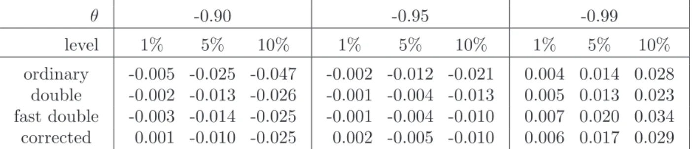
In order to emphasise just how small the size distortions are at conventional levels,Table 1

gives the actual numbers for n= 100, α= 0.01, 0.05, 0.10, and for θ =−0.90, -0.95, -0.99. Overall, it appears that the corrected bootstrap methods do improve on the ordinary bootstrap. It is striking how similar are the performances of all three of these methods. In particular, the error in the rejection probability (ERP) of the FDB, for which the

θ -0.90 -0.95 -0.99 level 1% 5% 10% 1% 5% 10% 1% 5% 10% ordinary -0.005 -0.025 -0.047 -0.002 -0.012 -0.021 0.004 0.014 0.028 double -0.002 -0.013 -0.026 -0.001 -0.004 -0.013 0.005 0.013 0.023 fast double -0.003 -0.014 -0.025 -0.001 -0.004 -0.010 0.007 0.020 0.034 corrected 0.001 -0.010 -0.025 0.002 -0.005 -0.010 0.006 0.017 0.029

Table 1: Size distortions of bootstrap tests, n=100

theoretical justification is rather weak, given that τ and µ∗ _{are by no means independent,}

is seldom any greater than that of the double bootstrap, and is often smaller. 7. Possible Extensions Let D(τ, µ) be defined by D(τ, µ) =R ³ Q∗¡R(τ, µ), µ¢, µ ´ . Then we can see from (21) that p∗

FDB(ω, µ) = D ¡

τ(ω, µ), µ(ω, µ)¢. If we can generate D(τ, µ) for arbitrary (τ, µ), we can readily generate the independent copies ofp∗

FDB needed to estimate the RP of the FDB test, and thus obtain a correctedP value for the fast double bootstrap.

In the case in which the space of DGPs is one-dimensional, we can generate D(·, µ) for a grid of values of µ, and use interpolation for arbitrary µ. For fixed µ, we proceed as follows. For i= 1, . . . , N,

• Generate τ∗

i and µ∗i as τ(ωi, µ) andµ(ωi, µ).

• Generate τ∗∗

i as τ(ω∗i, µ∗i). Theτ∗∗ are IID realisations of the distribution with CDF R∗_{(·, µ).}

• Sort the pairs (τ∗

i , µ∗i) in increasing order of the τi∗.

• Sort the τ∗∗ i in increasing order. • Estimateq∗ i ≡Q∗ ¡ R(τ∗ i, µ), µ ¢

as elementiof the sortedτ∗∗_{. Elementiis an estimate}

of thei/N quantile of the distribution with CDF R∗_{(·, µ), that is, ofQ}∗_{(i/N, µ). But,}

after sorting,τ∗

i estimates the i/N quantile of the distribution with CDFR(·, µ), and so i/N is an estimate of R(τ∗

i, µ).

• Estimate R¡Q∗_(R(τ∗

i, µ), µ), µ ¢

by the proportion of the τ∗ _{that are less than q}∗

i. This gives estimates of D(τ, µ) for the given µ and all the realised values τ∗

i. We repeat this for all the µ of our one-dimensional grid.

The next step is to generate the p∗

FDB(ωi, µ) = D(τi∗, µ∗i). Since we sorted the µ∗i along with the τ∗

i, they are still paired. For each of the µk, k = 1, . . . , K, of the K points of

the grid, we evaluate D(τ∗

i, µk) by simple linear interpolation. This is necessary because the realised τ∗

i are different for differentµk. However, for N large enough, the realisations should be fairly densely spread in the relevant region, and so linear interpolation should be adequate. However, since the experiment for each µk is rather costly, we cannot populate the space of the µ at all densely. Thus we prefer to estimate D(τ∗

i, µ∗i) by cubic-spline interpolation based on the D(τ∗

i, µk). It may be sensible to check that D(·, µ) is a smooth enough function of µ.

In the experiments done using this approach, N = 99,999 in the estimation of the grid of values of D(τ, µ), but only every 9th _{realisation was used to compute a realisation of} p∗

FDB(ω), for a total of 11,111 realisations. Computing time was still very long. The results are shown in Figure 6. where the estimated bootstrap discrepancy of the FDB is compared with the discrepancy as estimated by a brute-force simulation experiment. The two estimates are very similar. It is therefore quite possible to envisage a long computation in which the discrepancy of the FDB is bootstrapped, in order to obtain a corrected value, which should suffer from very little size distortion. A simulation experiment to investigate this would unfortunately be extremely costly, at least with today’s equipment.

0.02 0.04 0.06 0.08 0.10 −0.03 −0.02 −0.01 0.00 _... ..._... ..._... ... ..._... ..._... ..._... ... α Bootstrap discrepancy 0.02 0.04 0.06 0.08 0.10 −0.010 −0.005 0.000 _... ... ... ... ..._... ... ... ..._... ..._... ..._... ..._... ... α Bootstrap discrepancy n= 100, θ =−0.90 n= 100, θ =−0.95 0.02 0.04 0.06 0.08 0.10 0.00 0.01 0.02 0.03 ... ... ... ... ... ... ... ... _{Actual FDB} ... ... ... ... ... ... ... ... ... _{Simulated estimate} α Bootstrap discrepancy n= 100, θ=−0.99 Figure 6: Discrepancy of the FDB

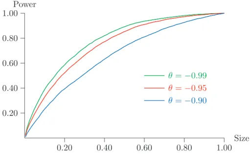
8. Power Properties

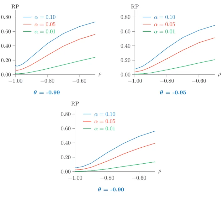
In this short section, the power of the (ordinary) bootstrap test is examined. Since its ERP is never very great, the rejection probability under DGPs that do not have a unit

−1.00 −0.80 −0.60 0.00 0.20 0.40 0.60 0.80 ... ... ... ... ... ... _{α = 0.01} ... ... ... ... ... ... ... ... ... ... ... _{α = 0.05} ... ... ... ... ... ... ... ... ... ... ... ... ... _{α = 0.10} ρ RP −1.00 −0.80 −0.60 0.00 0.20 0.40 0.60 0.80 ... ... ... ... ... _{α= 0.01} ... ... ... ... ... ... ... ... ... ... _{α= 0.05} ... ... ... ... ... ... ... ... ... ... ... ... ... _{α= 0.10} ρ RP θ = -0.99 θ = -0.95 −1.00 −0.80 −0.60 0.00 0.20 0.40 0.60 0.80 ... ... ... ... α= 0.01 ... ... ... ... ... ... ... ... ... α= 0.05 ... ... ... ... ... ... ... ... ... ... ... α= 0.10 ρ RP θ = -0.90

Figure 7: Power of the bootstrap test for n = 100

root is a reasonably good measure of the real power of the test. In this specific case, it is in fact possible to consider genuinely size-corrected power, because we have seen that the rejection probability under the null has its supremum when θ → −1.

In Figure 7, rejection probabilities are plotted for bootstrap tests at nominal levels of 0.01, 0.05, and 0.10, and for sample size n = 100, for DGPs that are ARMA(1,1) processes of the form

(1 +ρL)y= (1 +θL)ε, (22)

for various values of ρ and θ in the neighbourhood of -1; note that the DGP (13) that satisfies the null hypothesis is just (22) with ρ = −1. Whenever ρ = θ, (22) describes only one DGP, whatever the common value of the two parameters may be. This DGP generates a series y that is just white noise. In particular, it is identical to the limit of DGPs that satisfy the null hypothesis with ρ=−1 when θ→ −1. It is worth noting that, although a white-noise y might seem very distant from a process with a unit root, it is