Contents lists available atScienceDirect
Computers and Mathematics with Applications
journal homepage:www.elsevier.com/locate/camwaSoftware reliability analysis and assessment using queueing models
with multiple change-points
Chin-Yu Huang
a,∗, Tsui-Ying Hung
baDepartment of Computer Science, National Tsing Hua University, Hsinchu, Taiwan bCustomer Service Systems Laboratory, Chungwha Telecom Co., Ltd., Taipei, Taiwan
a r t i c l e i n f o
Article history:
Received 31 May 2009
Received in revised form 6 July 2010 Accepted 23 July 2010
Keywords:
Software reliability growth model (SRGM) Change-point
Software testing Debugging
Non-homogeneous Poisson process (NHPP)
a b s t r a c t
Over the past three decades, many software reliability growth models (SRGMs) have been proposed, and they can be used to predict and estimate software reliability. One common assumption of these conventional SRGMs is to assume that detected faults will be removed immediately. In reality, this assumption may not be reasonable and may not always occur. During debugging, developers need time to reproduce the failure, identify the root causes of faults, fix them, and then re-run the software. From some experiments or observations, the fault correction rate may not be a constant and could be changed at certain points as time proceeds. Consequently, in this paper, we will investigate and study how to apply queueing models to describe the fault detection and correction processes during software development. We propose an extended infinite server queueing model with multiple change-points to predict and assess software reliability. Experimental results based on real failure data show that the proposed model can depict the change of fault correction rates and predict the behavior of software development more accurately than traditional SRGMs.
©2010 Elsevier Ltd. All rights reserved.
1. Introduction
Software is a relatively new product (and design approach) compared to hardware-based systems. Most software engineers have always spent a lot of time and effort trying to figure out how to create reliable software with minimum errors. According to ANSI’s definition, software reliability is the probability of failure-free software operation for a specified period of time in a specified environment [1,2]. Software reliability mainly depends on the code that results from several intermediate processes that must be considered in the final analysis. Time and money can be saved when early reliability prediction is feasible and measurable. Over the past three decades, many non-homogeneous Poisson process (NHPP)-basedsoftware reliability growth models(SRGMs) have been proposed for estimating and assessing the reliability growth of products [3,4].
In general, SRGMs allow engineers to determine how software reliability varies with time during testing and help them decide when to stop testing [5]. SRGMs have been widely used in many practical applications [6–8]. The applications of SRGMs include important and safety-critical systems such as the shuttle’s on-board system software [9] and weapon systems [10]. In addition to ANSI/AIAA, SRGMs have also been adopted or recommended by a number of leading companies or research institutions, such as AT&T, North Telecom, Bell Canada, JPL and AFOTEC (the Air Force Operational Evaluation Center) [11–13]. Baumer et al. [14] used NHPP models to predict fault inflow in some large-scale software projects of Ericsson AB. According to their experiences, the concave NHPP models performed well in short-term predictions in iterative processes. NHPP models are still adopted in industry.
∗Corresponding author. Tel.: +886 3 5742972; fax: +886 3 5723694.
E-mail address:[email protected](C.-Y. Huang).
0898-1221/$ – see front matter©2010 Elsevier Ltd. All rights reserved. doi:10.1016/j.camwa.2010.07.039
Software reliability estimation is generally affected by three main factors: fault detection, fault removal, and operational profile. Fault(s) can be detected and moved when a program fails and a failure occurs during execution. One common assumption of most conventional SRGMs is that detected faults are immediately removed [15]. In reality, this assumption may not be reasonable and may not always occur. There is often a considerable time delay between finding a fault and fixing it, once the correction process has started. In the past decade, some researchers have discussed how to use queueing-based approaches to explain the debugging behavior and to allocate limited testing resources [16–20]. In the queueing-based approaches of modeling software reliability, detected faults and debuggers are usually regarded as customers and servers, respectively. The time between a customer entering the queue and leaving after service completion is considered to be the time needed to remove a bug.
In addition, most SRGMs typically assume that the rate of fault correction is a constant. In reality, this rate strongly depends on the skill of the debuggers, the difficulty of the problems (errors), debugging environments and tools, etc. Thus the fault correction rate may be neither constant nor smooth. Instead, it could be changed at certain moments in time called
change-points(CPs) [21,22]. In general, a CP is the time instant when a model’s parameter experiences a discontinuity in time. Zhao [23] suggested that, before the software is delivered to users, a CP may occur when the testing strategy and resource allocation are changed. That is, the running environment may change at that moment. The availability of testing facilities and other random factors can be the causes of the CPs. Some reliability CP models have been published in the past, such as the Weibull change-point model, the Jelinski–Moranda de-eutrophication model with a change-point and the Littlewood model with one change-point [23].
In this paper, we will propose an extended infinite server queueing model (EISQM) with multiple CPs. The proposed model can help managers and developers measure software reliability, and can understand the possible change of the fault correction rate. We also propose a method to locate the CP(s). That is, this method can greatly help engineers to estimate and provide inferences for the location of CP(s). The applicability of our proposed model will be demonstrated using two sets of real software failure data. Experimental results show that the proposed models give a better fit to the data sets and predict the future behavior well.
The remainder of this paper is organized as follows. Section2gives a review of some existing SRGMs. We further survey the application of queueing theory in software reliability modeling and discuss the problem of time lag between failure detection and fault correction processes in Section3. In Section4, we will show how to derive an EISQM with multiple CPs. We estimate the parameters of the proposed models based on real data sets, and compare the performance of the proposed models with a number of SRGMs in Section5. Finally, conclusions are given in Section6.
2. Review of some software reliability models
In the past three decades, many SRGMs have been proposed and studied [2,24]. For example, Musa et al. [1] focused on the study of the NHPP and further proposed the logarithmic Poisson execution time model. Another important model, the Schneidewind model, proposed by Schneidewind, is also a type of NHPP model [2,7,9]. The most important feature is that the applications of NHPP models are diverse and critical in practice. Both the logarithmic Poisson execution time model and the Schneidewind model are recommended by ANSI/AIAA. Among various models, NHPP models are very attractive. Xie [25] reported that NHPP models are simple and easy to use, and they are the type of software reliability model that is most widely applied. Besides, Farr and Lyu [2] also pointed out that the NHPP model has formed the basis for models using the observed number of faults per unit time group. But it should be noticed that there are no universally applicable SRGMs so far, i.e., no existing models can be trusted to provide accurate predictions of reliability in all situations. In the following, some widely used NHPP SRGMs are presented and discussed.
2.1. The Goel–Okumoto model
This model, first proposed by Goel and Okumoto [2,24], is one of the most popular and famous NHPP-based models. The assumptions of the Goel and Okumoto model are as follows.
1. The fault removal process follows the NHPP.
2. The software system is subject to failures at random times caused by faults remaining in the system.
3. The mean number of failures detected in the time interval (t
,
t+
∆t] is proportional to the mean number of faults remaining in the system.4. All faults are mutually independent and have the same chance of being detected.
5. When a failure is observed and a fault is detected, the detected fault will be removed immediately, and no new faults are introduced.
Based on the above assumptions, we have the following differential equation: dmd
(
t)
dt
=
b[a−
md(
t)
],
(1)wheremd
(
t)
is the expected number of faults detected by timet,ais the expected number of faults which will be eventuallydetected, andbis the fault detection rate. Solving Eq.(1)under the boundary conditionmd
(
0)
=
0, we haveEq.(2)is generally called the Goel–Okumoto model, and its mean value function (MVF) is exponential shaped. The failure intensity function is given by
λ
d(
t)
≡
dmd
(
t)
dt
=
abe−bt
.
(3)Goel reported that this model was applied to several internal projects developed within the Jet Propulsion Laboratory [26].
2.2. The Yamada delayed S-shaped model
The delayed S-shaped model was originally proposed by Yamada et al. [27] and was designed to capture the software fault removal phenomenon. They reported that the software failure detection process of this model can be viewed as a learning process since the software testers become more familiar with the testing environments and tools as time progresses. Thus the skills of testers will be gradually improved and then level off as the residual faults become more difficult to uncover [4]. It is also noticed that original Yamada delayed S-shaped model was developed for the analysis of fault isolation data; thus the testing process contains not only a fault detection process, but also a fault isolation process. There are some assumptions for this model [2,24].
(1) The fault removal process follows the NHPP.
(2) The software system is subject to failures at random times caused by faults remaining in the system.
(3) The mean number of failures detected in the time interval (t
,
t+
∆t] is proportional to the mean number of faults remaining in the system.(4) The proportionality of failure detection is constant.
(5) The mean number of faults isolated in the time interval (t
,
t+
∆t] is proportional to the current number of faults not isolated in the system.(6) The proportionality of fault isolation is constant.
(7) Each time a failure occurs, the fault which caused it is immediately removed, and no new faults are introduced. Based on the assumptions, the Yamada delayed S-shaped model can be formulated as
dmd
(
t)
dt
=
b× [
a−
md(
t)
]
,
(4)and
dmr
(
t)
dt
=
b2× [
md(
t)
−
mr(
t)
]
,
(5)wheremd
(
t)
is the cumulative number of faults detected up tot,mr(
t)
is the cumulative number of faults isolated up tot, andbandb2are the failure detection rate and fault isolation rate, respectively. Here we assume thatb2
6=
b. SolvingEqs.(4)and(5)under the boundary conditionmd
(
0)
=
mr(
0)
=
0, we havemd
(
t)
=
a(
1−
exp[−
bt]
),
(6) and mr(
t)
=
a 1−
bexp[−
b2t] −
b2exp[−
bt]
b−
b2.
(7)Ifb2is approximately the same asb, from L’Hospital’s Rule, Eq.(7)will become
mr
(
t)
=
a{
1−
(
1+
bt)
exp[−
bt]}
.
(8)Thus the failure intensity function is given by
λ
r(
t)
=
ab2te−bt.
(9)2.3. The inflection S-shaped model
The inflection S-shaped model was proposed by Ohba [28], and its underlying concept is that the observed software reliability growth becomes S-shaped if the faults in a program are mutually dependent, i.e., some faults are not detectable before some others are removed [4]. Note that, from Eqs. (1), (4) and (5), we can obtain the following differential equation [24]:
dmd
(
t)
dt
=
b(
t)
[a−
md(
t)
],
(10)whereb
(
t)
is the fault detection rate function. If we substituteb(
t)
=
b/(
1+
ce−bt)
into Eq.(10)and assume the initialconditionmd
(
0)
=
0, we obtain the MVFmd(
t)
as follows:md
(
t)
=
a
(
1−
e−bt)
2 4 6 8 10 12 14 16 20 40 60 80 100 120 140 Cumulative # of failures Detected Removed Open-remaining faults Time(weeks)
Fig. 1. Cumulative number of detected and corrected faults for Wu’s data set.
wherecrepresents the inflection factor. Eq.(11)is generally called the inflection S-shaped model and it solves a technical problem in the Goel–Okumoto model. Its failure intensity function is given by
λ
d(
t)
=
ab
(
1+
c)
e−bt(
1+
ce−bt)
2.
(12)Note that both the inflection S-shaped model and the Yamada delayed S-shaped model are the two most commonly used S-shaped NHPP models in the field of software reliability modeling.
3. Software testing, debugging, and change-points 3.1. Fault identification and correction
In general, software testing is the process of running a program on some predetermined input data and capturing the behavior and output data prior to delivery to the end users [29]. Practically, some faults may be easy to find and correct, but some faults may reside in non-executable parts of the code, such as the ELF header or string table. For example, faults located in the ELF header may cause the OS to load the program incorrectly and lead to segmentation faults. Faults in a string table may also link an unexpected library and abort the normal execution of the program. When collecting the failure data set, we have to take into account all faults in the whole software system. The faults in non-executable parts should be included as well. It should be noted that not all executable software faults will lead to failures.
On the other hand, debugging refers to the process of finding the root cause(s) of system failure and fixing the problem. Effective debugging is not a simple task because most detected faults may not be immediately obvious. In most cases, debugging during the testing phase remains manual, but debugging during the operational phase is very complicated and hard to implement [29]. In general, the process of removing faults can roughly be divided into three steps:fault detection,fault isolation, andfault correction[30]. Fault detection may be realized by inspection, software testing, and formal verification [30]. Once a fault is detected, the goal of fault isolation is to identify the location of the root cause of the error. This usually consists of two steps: gathering information to form a hypothesis, and testing the hypothesis. When the specific root cause is recognized, we can correct the fault accordingly [31].
It is noted that, in some cases, fault correction is not performed immediately, especially when problem determination involves multiple interacting software products [29]. Thus the debugging will be time consuming, and the time lag between failure detection and fault correction should not be ignored [15,32,33]. Shooman [34] discussed the fault generation phenomenon during debugging and assumed that the fault generation rate could be less than, greater than, or equal to the fault correction rate. He argued that the best way to formulate models for the generation and correction rate is to use studies of real experimental data.
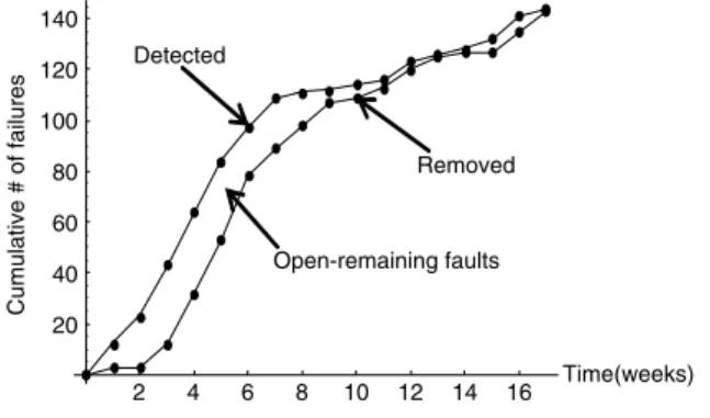
Littlewood’s Bayesian debugging model [35] assumed that each software failure may not contribute equally because the fault correction in the beginning of the testing phase will have more of an effect on the program than corrections taking place later. Musa et al. [1] proposed a basic execution time model that can be used to model the amount of limiting resources, such as failure identification personnel, failure correction personnel, or computer time. He reported a System T1 failure data set in [1]. From this data set, we can clearly see the time lag between fault detection and correction processes. Besides, Wu et al. [32] proposed some approaches to model both software fault detection and correction processes, and used an actual set of data to illustrate the modeling and reliability analysis procedure.Fig. 1depicts this data set, and it clearly indicates that the fault removal time is probably not negligible, because the number of removed faults lags far behind the total number of detected faults.
Finally, in addition to modeling approaches, researchers have recently studied how to use queueing-based approaches to explain the debugging behaviors in software development. For example, Wallace and Coleman [33] found that the most important factor in the fault correction modeling process was the time delay between failure detection and correction. They modeled this factor using the concept of a fault correction queueing service with an exponentially distributed delay—a
highly statistically significant empirical result based on data from the NASA space shuttle program. Yang [19] also proposed an infinite server queueing model to predict software reliability and to determine whether the software system is ready for release. He assumed that the number of debuggers is infinite so that the faults do not need to wait for service. Gokhale and Mullen [18] proposed a multi-priority queueing model for the software defect resolution process. They showed the utility of structuring the system asnindependent M/M/1 queues.
3.2. Change-points
Generally speaking, in the beginning of the testing phase, many faults can be discovered by inspection, and the failure detection rate depends on the fault discovery efficiency, the fault density, the testing effort, the inspection rate, and other factors. In the middle stage of the testing phase, the failure detection rate normally depends on other parameters such as the execution rate of CPU instructions, the failure-to-fault relationship, the code expansion factor, and the scheduled CPU hours per calendar day. Consequently, the failure detection rate can be calculated. We can engage this rate to track the progress of checking activities, to evaluate the effectiveness of test planning, and to assess the checking methods we adopted.
But in reality, during debugging, the fault correction rate strongly depends on the skill of the debuggers, the difficulty of errors, debugging environments and tools, etc. Thus the fault correction rate will probably be neither constant nor smooth, i.e., it may change at some moments in time called change-points (CPs). Practical experiences show that, during the fault correction period, the ability of debuggers or developers may change as time increases. Sometimes re-staffing can also be carried out to avoid wasting resources or missing a deadline. In engineering modern software, it is advisable to introduce new debugging tools that are fundamentally different from the methods used previously [1]. These tools could provide a steady improvement in software testing and productivity. Therefore, the timing of introducing new tools can be treated as a CP.
In general, a CP is the time instant when a model’s parameter experiences a discontinuity in time. That is, it is the time at which the parameter changes values. In recent years, a number of papers have addressed the problem of CPs in the research field of software reliability [36–40]. For example, Zhao [37] suggested that, before the software is released to field operation, a CP could occur when the testing strategy and resource allocation are changed. That is, the execution environment may change at that moment. The availability of testing facilities and other random factors can also be the causes of the CPs. Besides, testing and/or debugging effort may not be constant due to low personnel retention rates [41]. Durand and Gaudoin [39] considered that the assumption of continuous failure intensity is not realistic, since fault debugging could induce a discontinuity. Therefore, they proposed a framework of hidden Markov chains (HMCs) for the modeling of the failure and debugging processes of software. In the following, we will study and show how to derive an EISQM with multiple CPs to model software reliability.
4. Extended infinite server queueing models with multiple change-points
The assumptions of the proposed EISQ model with multiple CPs are given below [19,20]. (1) The software failure detection process follows the NHPP.
(2) The software is subject to failures at random times, caused by the manifestation of faults remaining in the system. (3) The mean number of failures detected in the time interval (t
,
t+
∆t] is proportional to the mean number of faultsremaining in the system.
(4) The fault removal time is non-negligible, so the number of faults removed lags behind the total number of failures detected.
(5) Each time a failure occurs, the fault that causes it will eventually be removed. Failure detection activity continues while faults are being removed, and fault removals do not affect the detection process. When a fault is removed, it will not introduce a new fault.
(6) The queueing model for describing failure detection and fault removal activities is an infinite server queue with NHPP arrival, and general service time distribution.
(7) The mean service rate of faults corrected (i.e., the fault correction rate) is not just a constant or in some case may be changed at some time moment
τ
called a CP.Let us first consider the case of an EISQM with a single CP (
τ
1). Basically,mr(
t)
can be obtained frommr(
0, τ
1] +
mr(τ
1,
t]
.Suppose that an arbitrary failure is detected at timex1
(
x1≤
τ
1)
; then the probability that the detected failure has beencorrected by time
τ
1is equal toG1(τ
1−
x1)
. Under this condition, we letqbe the probability that a failure is detected at time x1and the fault that caused this will be completely removed in(
x1, τ
1]
. From the total probability theorem [42], we havethe following.
P
{
time required for complete removal≤
τ
1−
x1∩
failure detected atx1}
=
P{
time required for complete removal≤
τ
1−
x1|
failure detected atx1}
×
P{
failure detected atx1}
.
(13)The probability that a fault is detected at timex1over the interval
(
0, τ
1]
is given by [43] P{
failure is detected at timex1} =
m0d
(
x1)
md(τ
1)
.
In this case, we have
q
=
Z
τ10
P
{
time required for complete removal≤
τ
1−
x1∩
failure detected atx1}
=
Z
τ1 0 G1(τ
1−
x1)
m0 d(
x1)
md(τ
1)
dx1.
(15)Thenmr
(
0, τ
1] =
md(
0, τ
1] ×
q, and the departure process over the time interval[
0, τ
1]
is given by mr(
0, τ
1] =
md(
0, τ
1] ×
q=
md(τ
1)
×
Z
τ1 0 G1(τ
1−
x1)
m0d(
x1)
md(τ
1)
dx1=
Z
τ1 0 G(τ
1−
x1)
0d(
x1)
dx1.
(16)Eq.(16)can be written as
mr
(
0, τ
1] =
Z
τ10
g1
(τ
1−
x1)
md(
x1)
dx1.
(17)Next,mr
(τ
1,
t]
is composed of correcting faults which are detected over the time interval(τ
1,
t]
and removing theopen-remaining (i.e., detected but not corrected) faults at time
τ
1. Suppose that an arbitrary failure is detected at time x2; then the probability that the detected (observed) failure has been corrected by timetis equal toG2(
t−
x2)
. Letrbe theprobability that a failure is detected at timex2and the fault causing the failure will be completely removed in
(
x2,
t]
. Thus, weobtain
P
{
time required for complete removal≤
t−
x2∩
failure detected atx2}
=
P{
time required for complete removal≤
t−
x2|
failure detected atx2}
×
P{
failure detected atx2}
.
(18)The probability that a fault is detected at timex2over the interval
[
τ
1,
t]
is given by P{
fault is detected at timex2} =
m0 d
(
x2)
md(
t)
−
md(τ
1)
.
(19) Similarly, we have r=
Z
t τ1P
{
time required for complete removal≤
t−
x2∩
fault detected atx2}
=
Z
t τ1 G2(
t−
x2)
m0 d(
x2)
md(
t)
−
md(τ
1)
dx2.
(20)Sincemr
(τ
1,
t] =
md(τ
1,
t] ×
r, the departure process of the faults which are detected over the interval(τ
1,
t]
is givenby
[
md(
t)
−
md(τ
1)
] ×
Z
t τ1 G2(
t−
x2)
m0d(
x2)
[
md(
t)
−
md(τ
1)
]
dx2=
Z
t τ1 G2(
t−
x2)
m 0 d(
x2)
dx2.
(21)Due to the debugging lag, the number of open-remaining faults at time
τ
1is equal tomd(τ
1)
−
mr(τ
1)
. Thus the numberof the open-remaining faults over the interval
(τ
1,
t]
is given by[
md(τ
1)
−
mr(τ
1)
] ×
G2(
t−
τ
1).
(22)From Eqs.(18),(21)and(22), we have
mr
(
t)
=
Z
τ1 0 g1(τ
1−
x1)
md(
x1)
dx1+
Z
t τ1 g2(
t−
x2)
md(
x2)
dx2+ [
md(τ
1)
−
mr(τ
1)
]
G2(
t−
τ
1),
(23)wheremd
(
0)
=
0,mr(
0)
=
0, andG1(
·
)
andG2(
·
)
are the cumulative distribution functions (CDFs) of the fault correction timeover the time interval
(
0, τ
1)
and(τ
1,
t)
, respectively. Here we letg1(
·
)
andg2(
·
)
be the probability distribution functions(PDFs) of the fault correction time over time interval
(
0, τ
1]
and(τ
1,
t]
, respectively. It is noted that, ifτ
1=
0, Eq.(23)canbe written as mr
(
t)
=
Z
t 0 g2(
t−
x2)
md(
x2)
dx2≈
Z
t 0 g(
t−
x)
md(
x)
dx.
(24)Similarly, for the EISQM with two CPs, we have mr
(
t)
=
md(τ
1)
×
Z
τ1 0 G1(τ
1−
x1)
m0d(
x1)
md(τ
1)
dx1+ [
md(τ
2)
−
md(τ
1)
]
Z
τ2 τ1 G2(τ
2−
x2)
m0d(
x2)
[
md(τ
2)
−
md(τ
1)
]
dx2+ [
md(τ
1)
−
mr(τ
1)
] ×
G2(τ
2−
τ
1)
+ [
md(
t)
−
md(τ
2)
]
×
Z
t τ2 G3(
t−
x3)
m0 d(
x3)
[
md(
t)
−
md(τ
2)
]
dx3+ [
md(τ
2)
−
mr(τ
2)
] ×
G3(
t−
τ
2)
=
Z
τ1 0 g1(τ
1−
x1)
md(
x1)
dx1+
Z
τ2 τ1 g2(τ
2−
x2)
md(
x2)
dx2+ [
md(τ
1)
−
mr(τ
1)
]
×
G2(τ
2−
τ
1)
+
Z
t τ2 g3(
t−
x3)
md(
x3)
dx3+ [
md(τ
2)
−
mr(τ
2)
] ×
G3(
t−
τ
2),
(25) where 0≤
τ
1≤
τ
2≤
t, andmd(
0)
=
mr(
0)
=
0.Finally, we have a generalized function of the EISQM with multiple CPs:
mr
(
t)
=
nX
i=0 mr(τ
i, τ
i+1]
=
nX
i=0Z
τi+1 τi gi+1(τ
i+1−
xi+1)
×
md(
xi+1)
dxi+1+
(
md(τ
i)
−
mr(τ
i))
×
Gi+1(τ
i+1−
τ
i)
,
(26) where 0≤
τ
i≤
τ
i+1≤
t,τ
0=
0,τ
n+1=
t, andmd(
0)
=
mr(
0)
=
0.It is noted that the number of hidden-remaining faults at timetis
mundF
(
t)
=
md(
∞
)
−
md(
t).
(27)Here we notice that mundF
(
t)
plus the total number of open-remaining faults will be the real estimated number offaults remaining in the software that could cause any unexpected failure or loss during operation. In practice, high-level managers have to decide when to release developed software to commercial market at appropriate times due to economic considerations. If the value ofmundF
(
t)
is out of control or far behind expectations, project managers, developers, qualityassurance engineers, and related users should meet together, and then discuss, prepare, and launch a corrective action to determine the root causes and decide whether extra testing/debugging efforts are needed to meet the user’s expectations.
Finally, Musa [1] have reported a real software fault data involving eight developers and 178 corrected faults to show that the correction time was exponentially distributed. In addition, Gokhale and Mullen [18] also reported that the correction time is exponentially distributed, no matter what the fault severity is. Thus we can assume that the correction time is an exponential distribution; that is,
G
(
x)
=
1−
e−µx.
(28)Thus we have
g
(
x)
=
µ
e−µx.
(29)It seems that this would be helpful for modeling the fault correction time during the phase of debugging. For example, from Eq.(23), we have mr
(
t)
=
Z
τ1 0 g1(τ
1−
x1)
md(
x1)
dx1+
Z
t τ1 g2(
t−
x2)
md(
x2)
dx2+ [
md(τ
1)
−
mr(τ
1)
] ×
G2(
t−
τ
1)
=
Z
τ1 0µ
1×
e−µ1(τ1−x1)×
md(
x1)
dx1+
Z
t τ1{
µ
2×
e−µ2(t−x2)×
m d(
x2)
dx2}
+ [
md(τ
1)
−
mr(τ
1)
] ×
(
1−
e−µ2(t−τ1)).
(30)5. Experimental studies and results
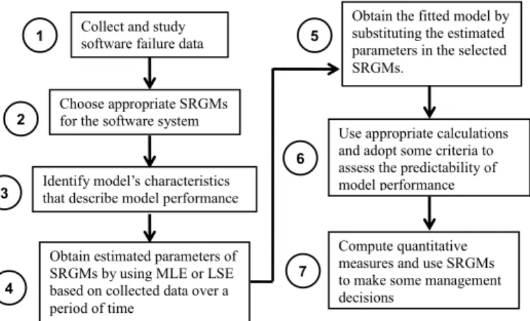
In order to evaluate the performance of our proposed models in Section4, the general guideline for performing experiments consists of several steps as outlined inFig. 2. It provides a context for presenting the use of software reliability models to assess and predict software reliability.
5.1. Failure data description
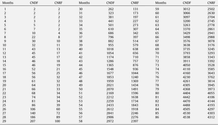
The first data set (DS1), seeTable 1, was presented by Musa [1, p. 413] for System T1 of the Rome Air Development Center project, and the failure data have been widely used and studied. System T1 is used for a real-time command and
Fig. 2. Steps for using SRGMs to predict software reliability. Table 1 DS1. Weeks CNDF CNRF Weeks CNDF CNRF 1 2 1 12 44 32 2 2 2 13 55 37 3 2 2 14 69 56 4 3 3 15 87 75 5 4 4 16 99 85 6 6 4 17 111 97 7 7 5 18 126 117 8 16 7 19 132 129 9 29 13 20 135 131 10 31 17 21 136 136 11 42 18
CNDF means cumulative number of detected failures and CNRF means cumulative number of removed failures.
control application. The size of the software is about 21,700 object instructions. It took 21 weeks and 9 programmers to complete the test. During the test phase, about 25.3 CPU h were consumed and 136 software faults were removed. The second data set (DS2), seeTable 2, was from the system P1 reported by Yang [19, p. 51]. The fault detection time and fault removal time of system P1 was about 86 months. The cumulative number of faults detected and removed was 4538 and 4312, respectively. FromTables 1and2, one clearly sees that the fault removal time is probably not negligible, because the number of faults removed lags far behind the total number of detected faults.
In general, software reliability studies are based on the application of different SRGMs to obtain various measures of interest. Various statistical tests have been published for identifying trends in grouped data or time series. Among the analytical tests, the Laplace test is the most commonly used, and it has been discussed in detail. Reliability growth can be analyzed by trend tests [2]. Note that blindly applying SRGMs may not lead to meaningful results when the trend indicated by the data differs from that predicted by the selected model. If the selected model is applied to the software failure data, and shows a trend in accordance with its original assumption, the results can be improved. Here we will calculate the Laplace trend factor. Let the time interval
(
0,
t]
be divided intokequal units of time. The Laplace factor can be defined as follows:l
(
k)
=
kP
i=1(
i−
1)
n(
i)
−
k−1 2 kP
i=1 n(
i)
s
k2−1 12 kP
i=1 n(
i)
,
(31)wheren
(
i)
is the number of faults observed during time uniti. Positive values ofl(
k)
indicate a decreasing software reliability, whereas negative values point out an increasing software reliability. If values ofl(
k)
vary between−
2 and+
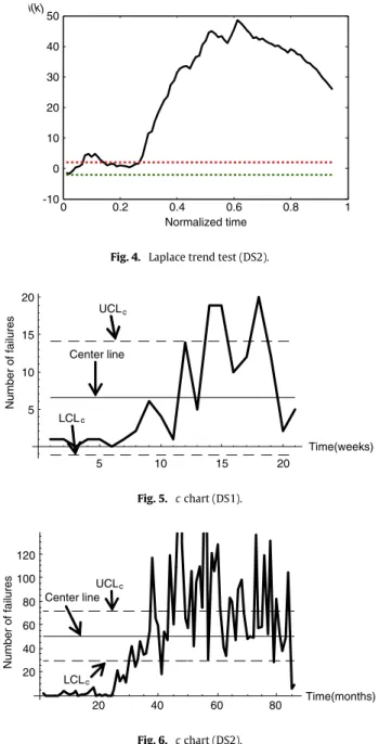
2, they represent a stable reliability. The analytic results for the two failure data sets are shown inFigs. 3and4. As seen fromFig. 3, we observe thatl(
k)
shows a steady decrease, indicating growth reliability. But for DS2, we can see fromFig. 4that, after 65% of the time, the value ofl(
k)
decreases. We can infer that the reliability will increase as time proceeds. In the case of reliability growth, our proposed models can be applied to predict the number of detected and corrected faults, and the failure intensity during the development phase.On the other hand, we propose using acchart to identify the location of the CPs. Acchart is a commonly used tool for monitoring a software process [44]. In acchart, control limits are estimated [45,46]. The parameters of thecchart are
Table 2 DS2.
Months CNDF CNRF Months CNDF CNRF Months CNDF CNRF
1 2 2 30 262 131 59 3012 2502 2 2 2 31 323 173 60 3066 2630 3 2 2 32 381 197 61 3097 2704 4 3 2 33 441 227 62 3200 2745 5 5 2 34 501 273 63 3263 2778 6 7 2 35 610 307 64 3370 2861 7 10 4 36 686 342 65 3429 2941 8 22 8 37 796 397 66 3498 2988 9 30 10 38 882 514 67 3576 3078 10 32 11 39 955 579 68 3638 3176 11 43 13 40 1018 638 69 3735 3245 12 45 17 41 1054 656 70 3793 3293 13 45 17 42 1174 710 71 3858 3343 14 46 18 43 1286 757 72 3911 3392 15 46 19 44 1365 876 73 4050 3528 16 52 21 45 1548 936 74 4110 3585 17 56 25 46 1677 1044 75 4160 3643 18 56 32 47 1853 1240 76 4230 3762 19 61 32 48 1959 1369 77 4261 3814 20 64 33 49 2021 1434 78 4305 3945 21 66 33 50 2070 1491 79 4368 3973 22 68 34 51 2169 1596 80 4404 4055 23 74 34 52 2212 1638 81 4442 4106 24 81 34 53 2259 1734 82 4470 4144 25 86 39 54 2433 1843 83 4488 4193 26 106 60 55 2612 1918 84 4505 4297 27 140 72 56 2841 2246 85 4530 4303 28 186 89 57 2906 2276 86 4538 4312 29 207 100 58 2972 2397 0 1 -9 -8 -7 -6 -5 -4 -3 -2 -1 l(k) -10 0.2 0.4 0.6 0.8 Normalized time
Fig. 3. Laplace trend test (DS1).
defined as [46] follows: UCLc
(
LCLc)
= ¯
C+
(
−
)
3p
¯
C,
(32) and C=
kP
i=1 n(
i)
k,
(33)whereUCLc,LCLcandC
¯
are the upper control limit, lower control limit, and centerline, respectively.Figs. 4and5give thecchart diagrams for DS1 and DS2, respectively.
There are some existing rules to detect unusual patterns and nonrandom behavior [46]. In this paper, if a single point falls outside theUCLcorLCLc, this can be treated as a CP. In addition, it is assumed that a CP is indicated when two out of
0 1 0 10 20 30 40 50 l(k) Normalized time -10 0.2 0.4 0.6 0.8
Fig. 4. Laplace trend test (DS2).
5 10 15 20 5 10 15 20 c UCLc Number of failures Center line LCL Time(weeks) Fig. 5. cchart (DS1). 20 40 60 80 20 40 60 80 c UCLc Number of failures 120 100 Time(months) Center line LCL Fig. 6. cchart (DS2).
For DS1, as we can see fromFig. 5, in the first 11 weeks of data, note that the values are below the centerline. But after the 11th week, the curve rises rapidly over the centerline. Thereafter, we assume that our first CP is located around at the 11th week. On the other hand, after the 18th week, the curve displays a rapid decrease inFig. 5. Therefore, we assume that the second CP is located at the 18th week.
For DS2, referring toFig. 6, we note that the values are below theLCLcin the first 32 months of data. But after the 32nd
month, the curve rises rapidly over the centerline. Consequently, the first CP is set at the 32nd month. It is also noticed that, around at the 64th month, two out of three values fall on the same side of the centerline. Thus we assume that the second CP is located around at the 64th month.
5.2. Performance comparison criteria
A model can generally be analyzed according to its retrodictive capability and predictive capability [2]. Since the data sets listed inTables 1and2are obtained as failure counts, we apply some criteria to compare various models’ performance, described as follows.
(1) Themean square of fitting error (MSE): In order to show quantitative comparisons for long-term predictions, we use the MSE because it provides a better-understood measure of the differences between actual and predicted values [2,24,47].
The MSE is generally defined as: MSE
=
kP
i=1[
m(
ti)
−
mi]
2 k,
(34)wherekis the size of the selected data set,miis the actual number of detected (or corrected) faults by timeti, andm
(
ti)
isthe estimated number of detected or corrected faults by timeti. Lower MSE means less fitting error and better performance.
(2) Thevarianceis defined as follows [48,49]:
Variance
=
v
u
u
u
t
kP
i=1(
mi−
m(
ti)
−
Bias)
2 k−
1,
(35) where Bias=
kP
i=1(
m(
ti)
−
mi)
k.
(36)The average of the prediction errors is called the prediction bias, and its standard deviation is often used as a measure of the variance in the predictions.
(3) Theroot mean square prediction error(RMSPE): This is defined as follows [49]: RMSPE
=
p
Variance2
+
Bias2.
(37)It is a measure of the closeness with which the model predicts the observation.
(4) TheTheil statistic(TS): The Theil statistic is the average total error percentage with regard to the actual values, and is defined as follows [50–52]: TS
=
v
u
u
u
u
u
u
t
kP
i=1[
m(
ti)
−
mi]
2 kP
i=1(
mi)
2×
100%.
(38)Lower values of TS represent better performance.
(5) Thepredictive validitycriterion: The capability of the model to predict failure behavior from present and past failure behavior is called predictive validity, which can be represented by computing therelative error(RE) for a data set [1]:
RE
=
m(
ti)
−
mimi
.
(39) Although there are various methods we can use to evaluate predictive validity, here we only choose the RE approach, since it is fairly easy and practical to apply. Musa [1] reported that, if a model is found to have the best predictive validity based on the failure data, it may yield the best values of other reliability quantities.
5.3. Model performance analysis
In this section, we will analyze the performance of our proposed models. Following the steps listed inFig. 1, if we choose some models to apply to a real software system, the next step is to estimate the models’ parameters. One well-known estimation technique isleast squares estimation(LSE). LSE minimizes the sum of the squares of the deviations between what is expected and what is actually observed. Becausemaximum likelihood estimation(MLE) tends to be biased [1] and LSE can produce unbiased results [25]; thus in this study we decided to use LSE to estimate the parameters of the proposed models.
Table 3summarizes the features of our selected models. Note that here we choose the inflection S-shaped model asmd
(
t)
formodels 1–3 because it provides a good fit to the selected data. However, it can easily be replaced by other existing SRGMs, such as the Goel–Okumoto model, the Yamada delayed S-shaped model, the Gompertz growth curve model, the logistic growth curve model, or the modified Duane model [2,4].
5.3.1. DS1
First, the estimated parameters of models 1–6 for the detected failures and corrected faults are listed inTables 4and5, respectively.Figs. 7and8depict the comparisons between the observed data and the data predicted by the MVFsmd
(
t)
andmr
(
t)
of proposed models 1–3, respectively. In addition, fromTable 5, we can see that the fault correction rate of models 2and 3 will change to that as shown inFig. 9. FromFig. 9, we find that the fault correction rate (i.e.,
µ
) of model 1 is a constant. However, the values ofµ
of models 2 and 3 are changed at some specified CP(s) during the fault correction period.Table 3
Summary of selected SRGMs.
Models Descriptions
#1 md(t): Inflection S-shaped model ISQM [4]
mr(t): Eq.(24)
#2 md(t): Inflection S-shaped model Proposed EISQM with 1 CP mr(t): Eq.(23)
#3 md(t): Inflection S-shaped model Proposed EISQM with 2 CPs
mr(t): Eq.(25)
#4 md(t): Eq.(6) Yamada delayed S-shaped (DSS) model
mr(t): Eq.(8)
#5 md(t): Eq.(11) Inflection S-shaped (ISS) model [2,4] mr(t): Eq.(11)
#6 md(t): Eq.(2) Goel–Okumoto (GO) model [2,4]
mr(t): Eq.(2) Table 4
Estimated parameters of models 1–6 for detected failures (DS1).
Models a b c #1 155.66 0.33 125.74 #2 155.66 0.33 125.74 #3 155.66 0.33 125.74 #4 137.20 0.156 – #5 155.66 0.33 125.74 #6 137.20 0.156 – Table 5
Estimated parameters of models 1–6 for removed failures (DS1).
Models a b c CPs µ #1 155.66 0.33 125.74 – µ=0.9 #2 155.66 0.33 125.74 τ1=11 µ1=0.293,µ2=0.255 #3 155.66 0.33 125.74 τ1=11,τ2=18 µ1=0.274,µ2=0.266, µ3=0.071 #4 208.00 0.10 – – – #5 186.82 0.30 169.75 – – #6 138.87 0.11 – – – 5 10 15 20 40 60 80 Actual data Number of failures 140 120 100 Models1-3 Time(weeks) 20
Fig. 7. md(t)of models 1–3 versus time for DS1.
5 10 15 20 40 60 80 Actual data Number of failures 140 120 100 20 Time(weeks) Model 2 Model 3 Model 1
Table 6
Comparison results of models 1–6 for removed faults.
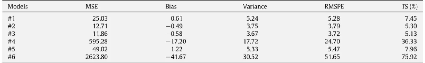
Models MSE Bias Variance RMSPE TS (%)
#1 25.03 0.61 5.24 5.28 7.45 #2 12.71 −0.49 3.75 3.79 5.30 #3 11.86 −0.58 3.67 3.72 5.13 #4 595.28 −17.20 17.72 24.70 36.33 #5 49.02 1.22 5.33 5.47 7.96 #6 2623.80 −41.67 30.52 51.65 75.92 11 18 21 0.293 0.2550.274 0.266 0.071 0.9 µ Time(weeks) Model 2 1st CP Model 1 2nd CP Model 3
Fig. 9. Fault correction rates of models 1–3 for DS1.
0.6 0.8 1 0.5 DSS GO 0.75 0.25 -0.25 -0.5 -0.75 Relative error Model 2 ISS Model 1 Normalized time 0.4 0.2 Model 3
Fig. 10. Relative error curves ofmr(t)of models 1–6 for DS1.
On the other hand, it is also noted that
µ
3of model 3 is less thanµ
1andµ
2. This means that the number of failuresdetected per unit time will decrease as time proceeds. Thus, a lower fault correction rate is obtained, and such a phenomenon is reasonable. In general, as time passes, the testing phase proceeds to the integration and system testing phases, and it becomes more difficult for testers to detect the remaining faults and for debuggers to quickly correct detected faults. In this case, the fault correction rate increases initially, and then decreases.Table 6gives the comparisons in terms of MSE, Bias, Variance, RMSPE, and TS. We can see that model 2 gives the lowest Bias, and that model 3 has the smallest values for MSE, Variance, RMSPE, and TS.
Finally,Fig. 10gives the graphical representation of the RE curves for different models against the normalized time. FromFig. 10, it seems that the proposed models 2 and 3 tend to be biased to the underestimation side when projection is made before 30% of the end of test time. But after 40% of the time, model 2 and model 3 project the future behavior well for this data set. It is also noted that some of the dispersion in the projection inFig. 10may be due to the sample size of failure data. Overall, we clearly see that the proposed models show increasingly accurate prediction when an increasing amount of historical data are used. FromTables 4–6andFigs. 7–10, we can see that the proposed models achieve a better goodness-of-fit than other SRGMs.
5.3.2. DS2
Similarly, we estimate the parameters of all selected models for the detected and corrected faults inTables 7and8. FromTable 8, we find that fault correction rates of models 2 and 3 are not constant, which reflects the variations of the fault correction rate during the fault correction process. InFigs. 11and12, we have plotted the comparisons between the observed failure data and the data estimated by the MVFsmd
(
t)
andmr(
t)
of proposed models 1–3, respectively. In addition, the faultTable 7
Estimated parameters of models 1–6 for detected faults (DS2).
Models a b c #1 4610.05 0.10 196.86 #2 4610.05 0.10 196.86 #3 4610.05 0.10 196.86 #4 4553.45 0.105 – #5 4610.05 0.100 196.86 #6 4553.45 0.105 – Table 8
Estimated parameters of models 1–6 for removed faults (DS2).
Models a b c CPs µ #1 4 610.05 0.100 196.86 – µ=0.164 #2 4 610.05 0.100 196.86 τ1=32 µ1=0.037,µ2=0.084 #3 4 610.05 0.100 196.86 τ1=32,τ2=62 µ1=0.022,µ2=0.094,µ3=0.018 #4 13 527.9 0.013 – – – #5 4 349.05 0.104 398.46 – – #6 4 318.66 0.100 – – – 20 40 60 80 4000 3000 2000 1000 Number of failures Actual data Models 1-3 Time(months)
Fig. 11. md(t)of models 1–3 versus time for DS2.
20 40 60 80 Number of failures 4000 3000 2000 1000 Model 1 Model 2 Model 3 Actual data Time(weeks)
Fig. 12. mr(t)of models 1–3 versus time for DS2.
32 62 86 0.164 0.037 0.084 0.022 0.094 0.018 µ Model 2 Model 1 1st CP Model 3 2nd CP Time(months)
Table 9
Comparison results of models 1–6 for removed faults (DS2).
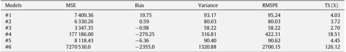
Models MSE Bias Variance RMSPE TS (%)
#1 7 409.36 19.75 93.17 95.24 4.03 #2 6 330.26 0.59 80.03 80.03 3.72 #3 3 347.35 −0.98 58.22 58.22 2.70 #4 177 186.00 −279.25 316.81 422.31 18.51 #5 8 118.43 −6.36 90.40 90.62 4.45 #6 7270 530.0 −2355.0 1320.88 2700.15 126.12 0.4 0.8 1 -1 1 2 3 GO Relative error ISS Model 1 DSS Model 3 Model 2 Normalized time 0.6 0.2
Fig. 14. Relative error curves ofmr(t)of models 1–6 for DS2.
in the starting and ending times, with maximum fault correction rate between the first and second CPs for model 3.Table 9
shows the comparisons in terms of MSE, Bias, Variance, RMSPE, and TS. We can also observe that model 2 gives the lowest value of Bias and that model 3 has the smallest value of MSE, Variance, RMSPE, and TS among the other models.
Finally, the graph inFig. 14depicts the relative errors for all selected models against the normalized time. Referring to
Fig. 14, we can clearly see that, after 20% of the time, the RE curves of model 2 and model 3 have better performances than the other models. Besides the models 2 and 3, we find that the other models tend to be biased to the overestimation side. As seen from these tables and figures, the proposed model give a better fit to DS2, and it predicts the future behavior well.
6. Conclusions
The fault correction process plays an important part in software development and reliability estimation. One major factor of fault correction modeling is the delay represented by the debugging time. In industries, software engineers have to update or revise the developed software many times during the life cycle of the software. In this case, a traditional SRGM may be good for one revision period rather than the whole life cycle. In this paper, we have shown how to apply a queueing-based model with multiple CPs to model the fault correction process. An EISQM with multiple CPs is proposed that can accurately reflect the variations in the fault correction rate and enhance the prediction and assessment of software reliability. Experiments are performed based on two real software failure data sets, and experimental results show that the proposed models give a better fit to the observed data. It is worthwhile noting that, by adding some extra parameters when modeling the fault correction process, the estimation becomes more tedious as more numerical calculations are involved. However, these additional calculations can be fully automated. Actually, based on the integrated theoretical foundation, the approaches presented in this paper offer a consistent, quantitative software reliability analysis scheme in both the testing and debugging phases.
Acknowledgements
The work described in this paper was supported by the National Science Council, Taiwan, under Grants NSC 97-2221-E-007-052-MY3, NSC 98-2221-E-007-067, and NSC 99-2220-E-007-022. The comments of the editor and anonymous referees are gratefully acknowledged.
References
[1] J.D. Musa, A. Iannino, K. Okumoto, Software Reliability, Measurement, Prediction and Application, McGraw-Hill, 1987. [2] M.R. Lyu, Handbook of Software Reliability Engineering, McGraw-Hill, 1996.
[3] C.Y. Huang, M.R. Lyu, S.Y. Kuo, A unified scheme of some non-homogenous poisson process models for software reliability estimation, IEEE Transactions on Software Engineering 29 (3) (2003) 261–269.
[4] M. Xie, Software Reliability Modeling, World Scientific Publishing Company, 1991.
[5] B. Yang, H. Hu, L. Jia, A study of uncertainty in software cost and its impact on optimal software release time, IEEE Transactions on Software Engineering 34 (6) (2008) 813–825.
[6] V.A. Almering, M.J.I.M. van Genuchten, P.J.M. Sonnemans, G. Cloudt, Using software reliability growth models in practice, IEEE Software 24 (6) (2007) 82–88.
[7] N.F. Schneidewind, A quantitative approach to software development using IEEE 982.1, IEEE Software 24 (1) (2007) 65–72.
[8] K. Kanoun, M. Bastos Martini, J. Moreira De Souza, A method for software reliability analysis and prediction application to the TROPICO-R switching system, IEEE Transactions on Software Engineering 17 (4) (1991) 334–344.
[9] N.F. Schneidewind, T.W. Keller, Application of reliability models to the space shuttle, IEEE Software 9 (4) (1992) 28–33.
[10] P. Carnes, Software reliability in weapon systems, in: Proceedings of the 8th International Symposium on Software Reliability Engineering: Case Studies, 1997, pp. 95–100.
[11] W.K. Ehrlich, K. Lee, R.H. Molisani, Applying reliability measurements: a case study, IEEE Software 7 (2) (1990) 56–64.
[12] W.D. Jones, Reliability models for very large software systems in industry, in: Proceeding of the 2nd International Symposium on Software Reliability Engineering, 1991, pp. 35–42.
[13] Recommended Practice for Software Reliability, R-013-1992, American National Standards Institute/American Institute of Aeronautics and Astronautics, 370 L’Enfant Promenade, SW, Washington, DC 20024, 1993.
[14] M. Baumer, P. Seidler, R. Torkar, R. Feldt, P. Tomaszewski, L. Damm, Predicting fault inflow in highly iterative software development processes: an industrial evaluation, in: Supplementary CD-ROM Proceedings of the 19th IEEE International Symposium on Software Reliability Engineering: Industry Track, 2008.
[15] C.Y. Huang, C.T. Lin, Software reliability analysis by considering fault dependency and debugging time lag, IEEE Transactions on Reliability 55 (3) (2006) 436–450.
[16] B. Luong, D.B. Liu, Resource allocation model in software development, in: Proceedings of the 47th IEEE Annual Reliability and Maintainability Symposium, 2001, pp. 213–218.
[17] S. Inoue, S. Yamada, A software reliability growth modeling based on infinite server queueing theory, in: Proceedings of the 9th ISSAT International Conference on Reliability and Quality in Design, 2003, pp. 305–309.
[18] S.S. Gokhale, R.E. Mullen, Queueing models for field defect resolution process, in: Proceedings of the 17th IEEE International Symposium on Software Reliability Engineering, Raleigh, North Carolina, 2006, pp. 353–362.
[19] K.Z. Yang, An infinite server queueing model for software readiness assessment and related performance measures, Ph.D. Dissertation, Department of Computer Engineering, Syracuse University, Syracuse, NY, 1996.
[20] C.Y. Huang, W.C. Huang, Software reliability analysis and measurement using finite and infinite server queueing models, IEEE Transactions on Reliability 57 (1) (2008) 192–203.
[21] C.Y. Huang, Performance analysis of software reliability growth models with testing-effort and change-point, Journal of Systems and Software 76 (2) (2005) 181–194.
[22] S. Inoue, S. Yamada, Optimal software release policy with change-point, in: Proceedings of 2008 IEEE International Conference on Industrial Engineering and Engineering Management, 2008, pp. 531–535.
[23] M. Zhao, Statistical reliability change-point estimation models, in: Handbook of Reliability Engineering, 2003, pp. 157–163. [24] H. Pham, Software Reliability, Springer-Verlag, 2000.
[25] M. Xie, Software reliability models—past, present and future, in: Recent Advances in Reliability Theory: Methodology, Practice and Inference, Birkhauser, Boston, 2000, pp. 323–340.
[26] A.L. Goel, Software reliability models: assumptions, limitations, and applicability, IEEE Transactions on Software Engineering 11 (12) (1985) 1411–1423.
[27] S. Yamada, M. Ohba, S. Osaki, S-shaped software reliability growth models and their applications, IEEE Transactions on Reliability 33 (4) (1984) 289–292.
[28] M. Ohba, Software reliability analysis models, IBM Journal of Research and Development 28 (4) (1984) 428–443. [29] B. Hailpern, P. Santhanam, Software debugging, testing, and verification, IBM Systems Journal 41 (1) (2002) 4–12. [30] M. Haug, E.W. Olsen, L. Consolini, Software Quality Approaches: Testing, Verification, and Validation, Springer, Berlin, 2001. [31] C. Kaner, J. Falk, H.Q. Nguyen, Testing Computer Software, 2nd ed., Wiley Computer Publishing, 1999.
[32] Y.P. Wu, Q.P. Hu, M. Xie, S.H. Ng, Modeling and analysis of software fault detection and correction process by considering time dependency, IEEE Transactions on Reliability 56 (4) (2007) 629–642.
[33] D. Wallace, C. Coleman, Application and improvement of software reliability models, Technical Report, Software Assurance Technology Center, SATC, NASA Goddard Space Flight Center, 2001.
[34] M.L. Shooman, Software Engineering: Design, Reliability, and Management, McGraw-Hill, 1983.
[35] B. Littlewood, A Bayesian differential debugging model for software reliability, in: Proceedings of the 4th IEEE International Computer Software and Applications Conference, 1980, pp. 511–517.
[36] F.Z. Zou, A change-point perspective on the software failure process, Software Testing, Verification and Reliability 13 (2) (2003) 85–93.
[37] J. Zhao, J. Wang, Testing the existence of change-point in NHPP software reliability models, Communications in Statistics—Simulation and Computation 36 (3) (2007) 607–619.
[38] P.K. Kapur, V.B. Singh, S. Anand, V.S.S. Yadavalli, Software reliability growth model with change-point and effort control using a power function of the testing time, International Journal of Production Research 46 (3) (2008) 771–787.
[39] J. Durand, O. Gaudoin, Software reliability modelling and prediction with hidden Markov chains, Statistical Modelling 5 (1) (2005) 75–93. [40] X. Li, M. Xie, S.H. Ng, Sensitivity analysis of release time of software reliability models incorporating testing effort with multiple change-points, Applied
Mathematical Modelling 34 (11) (2010) 3560–3570.
[41] J.D. Musa, Software Reliability Engineering: More Reliable Software, Faster and Cheaper, 2nd ed., McGraw-Hill, 2004.
[42] K.S. Trivedi, Probability and Statistics with Reliability, Queueing, and Computer Science Application, 2nd ed., John Wiley & Sons, 2002.
[43] K. Okumoto, Stochastic modelling for reliability and other performance measures of software systems with applications, Ph.D. Dissertation, Dept. of Industrial Engineering and Operations Research, Syracuse University, Syracuse, NY, 1979.
[44] R.S. Pressman, Software Engineering: A Practitioner’s Approach, International Edition, 7/e, McGraw-Hill, 2010.
[45] P. Jalote, A. Saxena, Optimum control limits for employing statistical process control in software process, IEEE Transactions on Software Engineering 28 (12) (2002) 1126–1134.
[46] W.A. Florac, A.D. Carleton, Measuring the Software Process: Statistical Process Control for Software Process Improvement, in: SEI Series in Software Engineering, Addison-Wesley, 1999.
[47] P.K. Kapur, D.N. Goswami, A. Bardhan, O. Singh, Flexible software reliability growth model with testing effort dependent learning process, Applied Mathematical Modelling 32 (7) (2008) 1298–1307.
[48] K. Pillai, V.S.S. Nair, A model for software development effort and cost estimation, IEEE Transactions on Software Engineering 23 (8) (1997) 485–497. [49] K. Srinivasan, D. Fisher, Machine learning approaches to estimating software development effort, IEEE Transactions on Software Engineering 21 (2)
(1995) 126–137.
[50] J.S. Armstrong, F. Collopy, Error measures for generalizing about forecasting methods: empirical comparisons, International Journal of Forecasting 8 (1) (1992) 69–80.
[51] P.L. Li, J. Herbsleb, M. Shaw, Forecasting field defect rates using a combined time-based and metrics-based approach: a case study of OpenBSD, in: Proceedings of the 16th IEEE International Symposium on Software Reliability Engineering, 2005, pp. 193–202.
[52] C.Y. Huang, C.T. Lin, Analysis of software reliability modeling considering testing compression factor and failure-to-fault relationship, IEEE Transactions on Computers 59 (2) (2010) 283–288.