DigitalCommons@University of Nebraska - Lincoln
Faculty Publications, Department of Statistics
Statistics, Department of
3-22-2012
Sample Size under Inverse Negative Binomial
Group Testing for Accuracy in Parameter
Estimation
Osval Antonio Montesinos-López
Universidad de Colima
, [email protected]
Abelardo Montesinos-López
Centro de Investigacion en Matematicas
Jose Crossa
Maize and Wheat Improvement Center
, [email protected]
Kent M. Eskridge
University of Nebraska-Lincoln
, [email protected]
Follow this and additional works at:
http://digitalcommons.unl.edu/statisticsfacpub
Part of the
Other Statistics and Probability Commons
This Article is brought to you for free and open access by the Statistics, Department of at DigitalCommons@University of Nebraska - Lincoln. It has been accepted for inclusion in Faculty Publications, Department of Statistics by an authorized administrator of DigitalCommons@University of Nebraska - Lincoln.
Montesinos-López, Osval Antonio; Montesinos-López, Abelardo; Crossa, Jose; and Eskridge, Kent M., "Sample Size under Inverse Negative Binomial Group Testing for Accuracy in Parameter Estimation" (2012).Faculty Publications, Department of Statistics. 24. http://digitalcommons.unl.edu/statisticsfacpub/24
Sample Size under Inverse Negative Binomial Group
Testing for Accuracy in Parameter Estimation
Osval Antonio Montesinos-Lo´pez1*, Abelardo Montesinos-Lo´pez2, Jose´ Crossa3*, Kent Eskridge4 1Facultad de Telema´tica, Universidad de Colima, Colima, Colima, Me´xico,2Departamento de Estadı´stica, Centro de Investigacio´n en Matema´ticas (CIMAT), Guanajuato, Guanajuato, Me´xico,3Biometrics and Statistics Unit, Maize and Wheat Improvement Center (CIMMYT), Mexico D.F., Mexico,4Department of Statistics, University of Nebraska, Lincoln, Nebraska, United States of America
Abstract
Background:The group testing method has been proposed for the detection and estimation of genetically modified plants (adventitious presence of unwanted transgenic plants, AP). For binary response variables (presence or absence), group testing is efficient when the prevalence is low, so that estimation, detection, and sample size methods have been developed under the binomial model. However, when the event is rare (low prevalence,0.1), and testing occurs sequentially, inverse (negative) binomial pooled sampling may be preferred.
Methodology/Principal Findings: This research proposes three sample size procedures (two computational and one analytic) for estimating prevalence using group testing under inverse (negative) binomial sampling. These methods provide the required number of positive pools (rm), given a pool size (k), for estimating the proportion of AP plants using the
Dorfman model and inverse (negative) binomial sampling. We give real and simulated examples to show how to apply these methods and the proposed sample-size formula. The Monte Carlo method was used to study the coverage and level of assurance achieved by the proposed sample sizes. An R program to create other scenarios is given in Appendix S2.
Conclusions:The three methods ensure precision in the estimated proportion of AP because they guarantee that the width (W) of the confidence interval (CI) will be equal to, or narrower than, the desired width (v), with a probability ofc. With the Monte Carlo study we found that the computational Wald procedure (method 2) produces the more precise sample size (with coverage and assurance levels very close to nominal values) and that the samples size based on the Clopper-Pearson CI (method 1) is conservative (overestimates the sample size); the analytic Wald sample size method we developed (method 3) sometimes underestimated the optimum number of pools.
Citation:Montesinos-Lo´pez OA, Montesinos-Lo´pez A, Crossa J, Eskridge K (2012) Sample Size under Inverse Negative Binomial Group Testing for Accuracy in Parameter Estimation. PLoS ONE 7(3): e32250. doi:10.1371/journal.pone.0032250
Editor:Ken R. Duffy, National University of Ireland Maynooth, Ireland
ReceivedAugust 16, 2011;AcceptedJanuary 25, 2012;PublishedMarch 22, 2012
Copyright:ß2012 Montesinos-Lo´pez et al. This is an open-access article distributed under the terms of the Creative Commons Attribution License, which permits unrestricted use, distribution, and reproduction in any medium, provided the original author and source are credited.
Funding:These authors have no support or funding to report.
Competing Interests:The authors have declared that no competing interests exist. * E-mail: [email protected] (OM); [email protected] (JC)
Introduction
To detect the presence of a rare event, thousands of individuals need to be tested, and the cost of such testing usually exceeds the available budget and staff. The pooling methodology (Dorfman method) was first proposed to save a significant amount of money when detecting soldiers with syphilis [1]. Significant cost savings were achieved by first testing a sample created by mixing blood from several people. If the sample tested positive, the blood from each individual in that pool would be retested; if the sample tested negative, all individuals in that pool were declared free of the disease [1]. Currently the Dorfman method is used for detecting and estimating the proportion of positive individuals in fields such as medicine [2,3,4,5], agriculture [6], telecommunications [7], and science fiction [8]. Most applications for detecting and estimating a proportion are developed using binomial sampling; however, Pritchard and Tebbs [9] have suggested that inverse (negative) binomial pooled sampling may be preferred when prevalencepis known to be small, when sampling and testing occur sequentially, or when positive pool results require immediate analysis—for
example, in the case of many rare diseases. Unlike binomial sampling, in this model the number of positive pools to be observed is fixeda priori, and testing is complete when the rth positive pool is reached [10].
George and Elston [11] recommended using geometric sampling when the probability of an event is small; they gave confidence intervals for the prevalence based on individual testing. Also, according to Haldane [12], using a binomial distribution may not provide an unbiased and precise estimate ofpwhenpis small (pƒ0:1). Lui [13] extended George and Elston’s work [11]
on the confidence interval (CI) by considering negative binomial sampling and showed that as the required number of successes increased, the width of the CI decreased. However, this extension was also under individual testing. Using negative binomial group testing sampling, Katholi [14] derived point and interval estimators ofp, obtained by both classical and Bayesian methods, and investigated their statistical properties.
Recently Pritchard and Tebbs [9] used maximum likelihood as a basis for developing three point and interval estimators for p
with Katholi’s [14] proposed point and interval estimators. Pritchard and Tebbs [10] extended their work to Bayesian point and interval estimation of the prevalence under negative binomial group testing. They used different distributions to incorporate prior knowledge of disease incidence and different loss functions, and derived closed-form expressions for posterior distributions and point and credible interval estimators [10]. However, until now sample size procedures under inverse (negative) binomial sampling for group testing have not been proposed.
In practice, pooling is a simple process; for example, if 40,000 plants are collected from the field, they could be tested one at a time for detecting unwanted transgenic plants (AP). If each test takes 15 minutes and costs US$12, then this project will take 10,000 hours and cost US$480,000. A shorter approach would be to smash 10 plants together and test this pooled sample [15]. This approach would take 1000 hours and cost US$48,000. Even greater savings are achieved with larger pool sizes. However, because the maximum likelihood estimator (MLE) of p under binomial [16] and negative binomial [9,10] group testing is biased to the right, then, on average, the MLE ofpoverestimates the true prevalence for any pool size (assuming a perfect diagnostic test); however, this bias is usually small whenpis small (p,0.1) [17]. In addition, if the diagnostic test is imperfect, a high rate of false positives is very likely. Thus, there are benefits and risks attached to the use of pooling methodology [15]. For this reason, it is important to choose the pool size with care in order to guarantee precision in the estimation process.
Under binomial group testing, some authors have proposed methods for determining the required sample size (number of required pools) to guarantee a certain level of power and/or precision [18,19,20,21]. Yamamura and Hino [18] and Herna´n-dez-Sua´rez et al. [19] developed sample size methods in terms of power considerations. This approach is consistent with the emphasis on hypothesis testing for inference, with results reported in terms of p-values. Montesinos-Lo´pez et al. [20,21] developed sample size procedures under the accuracy in parameter estimation
(AIPE) framework that guarantee narrow confidence intervals for estimating the parameter. The use of this approach is increasing, not only because the CIs ensure that the magnitude of the effect can be better assessed, but also because the effect in question can be readily identified by the reader. Furthermore, CIs also convey information about how precisely the magnitude of the effect can be ascertained from the data at hand [22]. Another advantage of the AIPE approach is that it treats the estimates (from pilot studies or literature review) used to determine the required sample size as random to guarantee that the desired CI width for estimating the parameter of interest is achieved, as originally planned [23].
However, under binomial group testing sampling when the prevalence is low, the calculated sample size sometimes does not contain any pools with the trait of interest (i.e., failure to detect and estimate AP). For this reason, inverse (negative) binomial sampling is a good alternative because each sample will contain the desired number of rare units and also the sample size is not a fixed quantity [12,9,10]. In binomial group testing, the number of required pools is treated as a fixed quantity, whereas under inverse (negative) binomial group testing, the pools are drawn one by one until the sample contains exactlyrpositive pools (here the number of positive pools is fixed).
Based on the previous findings, the purpose of the present study is to develop methods for determining sample size (number of positive pools) under inverse (negative) binomial group testing with the objective of increasing accuracy in the estimation of the population proportion. This research proposes methods for determining the required number of positive pools, with the aim of estimating the proportion of AP (p) using inverse (negative)
binomial group testing with a perfect test and fixed pool size (k) that will assure a narrow CI. Accuracy in the estimation ofpis achieved because CI width is considered stochastic and thus treated as a random variable. The methods used for achieving the objectives of the present research are: point and interval estimation for the population proportion, delta method, and central limit theorem. We provide an R program that reproduces the results presented in this study and makes it easy for the researcher to create other scenarios.
Materials and Methods
Suppose thatYi~yirepresents the number of pools tested until
the first positive pool is detected andY1,Y2,. . .,Yrare observed
to obtain the rth positive pool. Therefore, Yi has a geometric
distribution. Therefore, the overall number of pools that are tested to findrpositive pools is equal toT~Pr
i~1Yi. In what follows,
we shall denote the size of the pools collected ask and assume equal pool size; the prevalence of infection is denoted byp, the number of pools tested to find one positive pool isYi~yi, and the
number of times this experiment is carried out is denoted byr. It is important to mention that in this paper we consider that: (i) the sample size is the value ofrthat represents the number of positive pools required to stop the sampling and testing process, and (ii) the overall number of pools tested is the value ofT~Pr
i~1Yi. If the
prevalence of infection isp, then the probability that a pool of size
ktests positive isP~1{(1{p)k. Therefore, the sufficient sta-tisticsT~Pr
i~1Yi follows a negative binomial distribution (nib)
with waiting parameterrand success probabilityP~1{(1{p)k
[9,10,14]. According to Pritchard and Tebbs [9,10] and Katholi [14], the maximum likelihood estimate (MLE) ofpusing inverse (negative) binomial group testing is
^ p p~1{ 1{r T 1=k ð1Þ
wherekis the pool size andris the fixed required number of positive pools. This MLE ofpfor inverse (negative) binomial group testing with groups of equal size assumes a perfect diagnostic test. On the other hand, the variance of^ppaccording to Pritchard and Tebbs [9,10] and Katholi [14] is given byV(^pp)~ 1{(1{p) k 2 rk2(1{p)k{2 ~ P2(1{P)(2=k){1 rk2 .
According to Pritchard and Tebbs [9], the corresponding Wald CI is as follows: pL~^pp{Z1{a=2 ffiffiffiffiffiffiffiffiffiffi ^ V V(^pp) q pU~^ppzZ1{a=2 ffiffiffiffiffiffiffiffiffiffi ^ V V(^pp) q ð2Þ
where Z1{a=2 is the 1{a=2 quantile of the standard normal
distribution, and ^pp is the MLE estimated from Eq. (1). This approximation of the CI is easy to calculate and allows deriving closed-form sample size formulas. However, when r is small, the normal approximation for MLE is doubtful; in such cases, the Wald-type CI often produces negative endpoints. In addition, the coverage probability of the CIs constructed by Wald-type CIs is often smaller
than100(1{a)%.
Derivation of the sample size formula for detecting transgenic plants The quantity Z1{a=2 ffiffiffiffiffiffiffiffiffiffi ^ V V(^pp) q
(added and subtracted from the observed proportion,^pp) in Eq. (2) is defined asW/2(whereWis
the full width of the CI; W or W/2 can be set a priori by the researcher depending on the desired precision). The observed CI width for any realization of a confidence interval (from Eq. 2) can be expressed as: W~2Z1{a=2 (1{(1{^pp))k ffiffi r p k(1{^pp)k=2{1 ~2Z1{a=2 ffiffiffiffiffiffiffiffiffiffiffiffiffiffiffiffiffiffiffiffiffiffiffiffiffiffiffiffiffiffiffiffi ^ P P2(1{PP^)(2=k){1 rk2 s ð3Þ
Letvbe the desired CI width; then the basic AIPE approach seeks to find the minimum sample size so that the expected CI width is sufficiently narrow [24,25]. In other words, the AIPE approach seeks the minimal sample size so thatE(W)ƒv. The problem is that the
expected CI width is an unknown quantity, although it can be approximated. AsPP^~1=TTr, whereTTr~Pri~1Yi=r, the observed
width,W, is a function ofh(TTr)~ ffiffiffiffiffiffiffiffiffiffiffiffiffiffiffiffiffiffiffiffiffiffiffiffiffiffiffiffiffiffiffiffiffiffiffiffiffiffiffiffiffiffiffiffiffiffiffiffi 1{1=TTr ð Þ2=k{1ð1=TTrÞ2 k2 s . Since the distribution ofh(TTr)is unknown, it is not possible to obtain an
analytic solution forE(W). An alternative is to use the delta method to derive the asymptotic distribution of h(TTr). From Result 1 in
Appendix S1, we have that
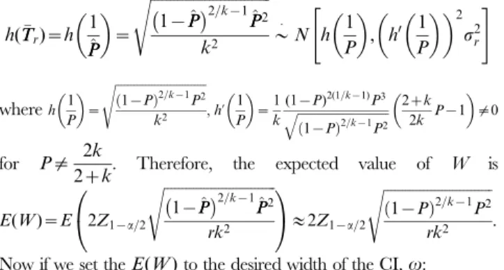
h(TTr)~h 1 ^ P P ~ ffiffiffiffiffiffiffiffiffiffiffiffiffiffiffiffiffiffiffiffiffiffiffiffiffiffiffiffiffiffiffi 1{PP^ 2=k{1^ P P2 k2 s *: N h 1 P , h0 1 P 2 s2r " # whereh 1 P ~ ffiffiffiffiffiffiffiffiffiffiffiffiffiffiffiffiffiffiffiffiffiffiffiffiffiffiffiffiffiffi 1{P ð Þ2=k{1P2 k2 s ,h’ 1 P ~1 k (1{P)2(1=k{1)P3 ffiffiffiffiffiffiffiffiffiffiffiffiffiffiffiffiffiffiffiffiffiffiffiffiffiffiffiffiffiffi 1{P ð Þ2=k{1P2 q 2zk 2k P{1 =0 for P= 2k
2zk. Therefore, the expected value of W is E(W)~E 2Z1{a =2 ffiffiffiffiffiffiffiffiffiffiffiffiffiffiffiffiffiffiffiffiffiffiffiffiffiffiffiffiffiffiffi 1{PP^ 2=k{1^ P P2 rk2 s 0 @ 1 A&2Z1{a=2 ffiffiffiffiffiffiffiffiffiffiffiffiffiffiffiffiffiffiffiffiffiffiffiffiffiffiffiffiffiffi 1{P ð Þ2=k{1 P2 rk2 s . Now if we set theE(W)to the desired width of the CI,v:
v~2Z1{a=2 ffiffiffiffiffiffiffiffiffiffiffiffiffiffiffiffiffiffiffiffiffiffiffiffiffiffiffiffiffiffi 1{P ð Þ2=k{1P2 rk2 s ð4Þ
Solving forr, Eq. (4) yields the following formulation:
rp~ 4Z2 1{a=2 1{(1{p) k 2 v2k2(1{p)k{2 ~4Z 2 1{a=2P2(1{P) (2=k){1 v2k2 ð5Þ
Note that ifk~1, Eq. (5) reduces to the formula derived by Lui [13]
rp~
4Z2
1{a=2p2(1{p)
v2
" #
. However, Eq. (5) requires the population value of p, which is unknown and in practice is replaced by an estimation of the true proportion. Eq. (5) finds the required sample size for achieving an expected CI width,E(W), that is sufficiently narrow for estimating the proportion of AP using pools; however, this does not guarantee that for any particular CI, the observed expected CI width,E(W), will be sufficiently narrow, because the expectation only approximates the mean CI width. Kelley and Rausch [25] state that this issue is similar to the case where a mean is estimated from a normal distribution; although the sample mean is an unbiased estimator of the population mean, the sample mean will almost certainly be smaller or larger than the population value. This is because the sample mean is a continuous random variable, as is the CI width, due to the fact that both are based on random data.
Thus, approximately half of the time, the computed confidence interval will be wider than the desired (specified) width [25].
Since Eq. (3) uses an estimate ofp,the CI width (W) is a random variable that will fluctuate from sample to sample. This implies that, using rp from Eq. (5), less than 50% of the sampling
distribution ofWwill be smaller thanv(see the third column in Table 1). To demonstrate this, we need to calculate the probability of obtaining a CI width that is smaller than the specified value (v). This can be computed as:
P(Wƒv)~ X? t~rp I(wt,t) t{1 rp{1 1{(1{p)k rp (1{p)k t{rp
whereI(wt,t)is an indicator function showing whether or not the
actual CI width calculated using Eq. (3 ) is #v, p is the true population proportion and rp is the sample size obtained using
equation (5). To avoid possible computer limitations, the above probability can be approximated by the following:
P(Wƒv)~ Xt t~rp I(wt,t) t{1 rp{1 1{(1{p)k rp (1{p)k t{rp ð6Þ
wheret~rp,rpz1,rpz2,. . .,t, andW is considered a random
variable because the exact value ofpis not known andtis the
value that satisfies P(Tƒt)~0:9999; we use this value of t
because in the R package summing to infinity is not possible.
Degree to which the sample size is underestimated using Eq. 5
To show the degree to whichrpis underestimated using Eq. (5),
we give an example (Table 1A) in which Eq. (6) is used to calculate
P(Wƒv), that is, the probability thatWwill be smaller than, or
equal to, the desired CI width (v) for a given valuerp(number of
positive pools) obtained using Eq. (5). The numerical example in Table 1 is given for several values of the population proportion (p) for a CI of 95%, k~25, and for a desired width ofv~0:007. Table 1A presents the preliminary sample sizerpcomputed with
Eq. (5), and three other increments computed asrm10~rpz10,
rm20~rpz20, and rm40~rpz40. For each sample size, the
probability thatWis smaller than the specified value (v~0:007),
P(Wƒv), is calculated using Eq. (6). This is done to show that the
required number of positive pools for the proportion (rp, second
column in Table 1A) computed using Eq. (5) has a probability of around 0.50 thatWƒv~0:007(third column in Table 1A). For
example, whenp~0:0125, the preliminary sample size (rp) is 49
and the probability of obtaining a Wƒv~0:007 is 0.4825564.
Withp~0:02,rp~126, we can only be 49.235% certain thatW
will beƒv~0:007. When the number of pools increases by 10
(rm10, fourth column, Table 1A) or by 20 (rm20, sixth column,
Table 1A), the probability P(Wƒv~0:007) increases. For
example, when p~0:0125, there are rm20= 69 units (pools) in
the sample with P(Wv0:007)~0:9091713; for rm40= 89 pools
in the sample, the P(Wv0:007)~0:9962656. Thus, results of
Table 1A show that in order to ensure a highP(Wƒv~0:007), a
bigger sample size (number of positive pools) than the preliminary one (rp) calculated using Eq. (5), is required. Also, we see in
Table 1A that 8 times out of 9 the preliminary sample size (number of positive pools) resulting from using Eq. (5) produces a
P(Wƒv)v0:50, that is, 88.89% of the time P(Wƒv~0:007)
was lower than 50%.
Forp~0:005, and a different combination of values ofkandr
values ofr, the percentage of times that the MLE ofpis larger than the population proportion is lower. These results also show that the level of underestimation of the required number of pools (rp)
caused by the use of Eq. (5) is important and is mainly due to the fact that half of the time the population proportionpwill be lower than the estimated proportion^pp(Table 1B);thus the obtained CI width (W) will be larger than the specifiedvabout more than half of the time. However, the expected value of the computedWis the value specified a priori (v), provided the correct value of the population variance is used. Therefore, the use of Eq. (5) will ensure that the desired width(v)for the CI will be obtained less than 50% of the time, that is,P(Wƒv)v0:5. The values of the
Mean Square Error (MSE) for p~0:005and different combina-tions ofkandr(Table 1C) indicate MSE increases for lower values ofr, however, no values ofkseem to guarantee low bias.
Since Eq. (5) underestimates the required number of pools, in the following section, we propose three new methods to estimate the optimum sample size (two computational and one analytic).
Computational optimum sample size estimation–methods 1 and 2
The optimal sample size is the smallest integer value (rm) such
that P(Wƒv)~ Xt t~rm I(wt,t) t {1 rm{1 1{(1{p)k rm (1{p)k t{rm §cð7Þ
whererm will start with a minimal sample size, say r0~1, and
I(wt,t)is an indicator function showing whether or not the actual
CI width (W) is #v. The CI width will be calculated as
wt~pU{pL. We determined that method 1 is when an exact
100(1{a)% CI for pis used, and method 2 is when the CI is
computed using the Wald CI (Eq. 2) and Eq. (7), which we call the computational Wald procedure.
The CI used for the exact method (method 1) is the Clopper-Pearson CI, as explained in the following. When equal pool sizesk
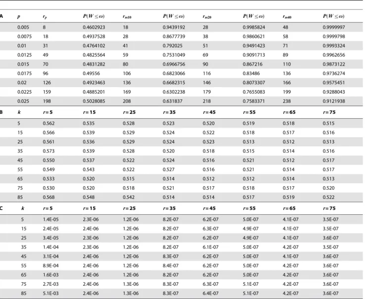
Table 1.Underestimation of the sample size given by using Eq. (5) (Table 1A).
A p rp P(Wƒv) rm10 P(Wƒv) rm20 P(Wƒv) rm40 P(Wƒv) 0.005 8 0.4602923 18 0.9439192 28 0.9985824 48 0.9999997 0.0075 18 0.4937528 28 0.8677739 38 0.9860621 58 0.9999798 0.01 31 0.4764102 41 0.792025 51 0.9491423 71 0.9993324 0.0125 49 0.4825564 59 0.7531049 69 0.9091713 89 0.9962656 0.015 70 0.4831282 80 0.6966756 90 0.867216 110 0.9873122 0.0175 96 0.49556 106 0.6823066 116 0.83486 136 0.9736274 0.02 126 0.4923463 136 0.6682315 146 0.8073307 166 0.9575451 0.0225 159 0.4885201 169 0.6302238 179 0.7655083 199 0.9288043 0.025 198 0.5028085 208 0.631837 218 0.7583371 238 0.9121938 B k r= 5 r= 15 r= 25 r= 35 r= 45 r= 55 r= 65 r= 75 5 0.562 0.535 0.528 0.523 0.520 0.519 0.518 0.515 15 0.566 0.539 0.529 0.524 0.522 0.518 0.517 0.516 25 0.561 0.536 0.529 0.524 0.523 0.513 0.512 0.513 35 0.573 0.539 0.528 0.520 0.518 0.515 0.514 0.516 45 0.550 0.537 0.522 0.524 0.516 0.521 0.512 0.517 55 0.549 0.543 0.522 0.527 0.516 0.521 0.514 0.517 65 0.533 0.520 0.515 0.514 0.512 0.512 0.514 0.513 75 0.530 0.520 0.518 0.521 0.517 0.518 0.517 0.520 85 0.568 0.548 0.542 0.514 0.514 0.517 0.519 0.522 C k r= 5 r= 15 r= 25 r= 35 r= 45 r= 55 r= 65 r= 75
5 1.4E-05 2.3E-06 1.2E-06 8.2E-07 6.2E-07 5.0E-07 4.1E-07 3.5E-07
15 2.4E-05 2.4E-06 1.2E-06 8.2E-07 6.3E-07 4.9E-07 4.1E-07 3.5E-07
25 3.4E-05 2.3E-06 1.2E-06 8.2E-07 6.2E-07 4.9E-07 4.1E-07 3.6E-07
35 1.4E-04 2.3E-06 1.2E-06 8.2E-07 6.1E-07 5.0E-07 4.2E-07 3.5E-07
45 3.1E-04 2.4E-06 1.2E-06 8.3E-07 6.2E-07 5.0E-07 4.1E-07 3.6E-07
55 8.9E-04 2.4E-06 1.2E-06 8.4E-07 6.2E-07 5.0E-07 4.2E-07 3.6E-07
65 1.6E-03 2.4E-06 1.2E-06 8.2E-07 6.2E-07 5.0E-07 4.2E-07 3.6E-07
75 2.7E-03 2.4E-06 1.3E-06 8.3E-07 6.3E-07 5.1E-07 4.2E-07 3.6E-07
85 5.1E-03 2.4E-06 1.3E-06 8.3E-07 6.4E-07 5.1E-07 4.2E-07 3.6E-07
Table 1A. Preliminary sample size (rp, number of required positive pools) for estimating the population proportion, computed with Eq. (5) and three sample size increments
(rm10~rpz10,rm20~rpz20, andrm40~rpz40) with their corresponding probability that the confidence interval width(W)is smaller than the specified value (v~0:007),
P(Wƒv)computed with Eq. (6). For a 95% CI andk~25,v~0:007is the desired CI width.P(Wvv)is the probability that (W) is smaller than the specified value
(v~0:007) calculated using Eq. (6). Table 1B. Proportion of times the MLE ofpis greater than the population proportionp~0:005for different combinations of values ofk
andrthat produce simulated 40, 000 samples. Table 1C. Mean Square Error for 40, 000 simulated samples withp~0:005and different values ofkandr. doi:10.1371/journal.pone.0032250.t001
are used,T*nib(rm,P), whereP~1{(1{p)k. Using the
relation-ship between the negative binomial distribution and the incomplete beta function, Lui [13] derived an exact interval forP. The lower and upper confidence limits arePL~B1{a=2,rm,t{rmz1andPU~Ba=2,rm,t{rm,
respectively, wheret~Pr
i~1yiandBa,a,b denotes theaquantile
of the two-parameter beta distribution [9]. Thus an exact
100(1{a)%CI for p can be obtained by suitably transforming
the endpoints of the Pinterval, i.e.,pU~1{ 1{Ba=2,rm,t{rm
1=k
and pL~1{ 1{B1{a=2,rm,t{rmz1
1=k
[9]. Also, this interval forp
can be formed using the relationship between the negative binomial and F distribution, in this casePL~ 1ztzrm1F1{a=2, 2(tz1), 2rm
h i{1 and PU~ rm t Fa=2, 2rm, 2t 1zrm t Fa=2, 2rm, 2t
, where Fa,a,b denotes the upper a
quantile of the two-parameter F distribution. Again, an exact
100(1{a)%CI forpispU~1{ 1{ rm t Fa=2, 2rm, 2t 1zrm t Fa=2, 2rm, 2t 0 B @ 1 C A 1=k and pL~1{ 1{ 1z tz1 rm F1{a=2, 2(tz1), 2rm {1!1=k [26]. This last version of the Clopper-Pearson CI has the advantage that the exact CI for p can be calculated by hand using standard F tables.
In methods 1 and 2, we start with a minimal sample size, say r0, and increase the initial number of pools (rm) by one
unit, recalculating Eq. (7) each time, until the desired degree of certainty (c) is achieved; this will produce a modified number of pools (rm) that assures, with a probability§c, that theWwill
be no wider than v. In other words, rm ensures that the
researcher will have approximately 100c percent certainty that the computed CI will have the desired width or smaller. For example, if the researcher requires 90% confidence that the obtained W will be no larger than the desired width (v), (1{c) would be defined as 0.10, and there would be only a 10% chance that the CI width, around^pp, would be larger than specified (v) [24,27].
Contrary to Eq. (5) above, the computational sample size proposed by Eq.(7) with methods 1 and 2 considers^ppas a random variable and gives a non-closed-form solution for computing a minimum sample size (rm) that guarantees thatWis smaller than,
or equal to, vwith a probability of at least c. In the following section, we propose a closed-form analytic method for determining the optimal sample size (number of positive pools required) that uses a single formula which assures the estimation of a narrow confidence interval.
Analytic optimum sample size estimation–method 3
The CI width using the Wald interval for p is
W~2Z1{a=2 ffiffiffiffiffiffiffiffiffiffi ^ V V(^pp) q
, and W must be smaller than a specified value (v) with probability (c). Therefore, the optimal sample size is defined as being the smallest integer value (rm) such that
P(Wƒv)~P 2Z1{a=2 ffiffiffiffiffiffiffiffiffiffiffiffiffiffiffiffiffiffiffiffiffiffiffiffiffiffiffiffiffiffiffi 1{PP^ 2=k{1^ P P2 rmk2 s ƒv 2 4 3 5§c ð8Þ
From Result 2 in Appendix S1, for fixed v, the number of required positive pools with method 3 is given by
rm~ h 1 P z ffiffiffiffiffiffiffiffiffiffiffiffiffiffiffiffiffiffiffiffiffiffiffiffiffiffiffiffiffiffiffiffiffiffiffiffiffiffiffiffiffiffiffiffiffiffiffiffiffiffiffiffiffiffiffiffiffiffiffiffiffiffiffiffiffiffiffiffiffiffiffiffi h 1 P 2 z 2v Z1{a=2 Zch’ 1 P ffiffiffiffiffiffiffiffiffiffiffi 1{P P2 r s v Z1{a=2 0 B B B B @ 1 C C C C A 2 ~ ffiffiffiffiffiffiffiffiffiffiffiffiffiffiffiffiffiffiffiffiffiffiffiffiffiffiffiffiffiffi 1{P ð Þ2=k{1P2 k2 s z ffiffiffiffiffiffiffiffiffiffiffiffiffiffiffiffiffiffiffiffiffiffiffiffiffiffiffiffiffiffiffiffiffiffiffiffiffiffiffiffiffiffiffiffiffiffiffiffiffiffiffiffiffiffiffiffiffiffiffiffiffiffiffiffiffiffiffiffiffiffiffiffiffiffiffiffiffiffiffiffiffiffiffiffiffiffiffiffiffiffiffiffiffiffiffiffiffiffiffiffiffiffiffiffiffiffiffiffiffiffiffiffiffiffiffiffiffiffiffiffiffiffiffiffiffiffiffiffiffiffiffiffiffiffiffiffiffiffiffiffiffiffi 1{P ð Þ2=k{1P2 k2 z 2v Z1{a=2 Zc 1 k (1{P)2(1=k{1)P3 ffiffiffiffiffiffiffiffiffiffiffiffiffiffiffiffiffiffiffiffiffiffiffiffiffiffiffiffiffiffi 1{P ð Þ2=k{1P2 q 2zk2k P{1 ffiffiffiffiffiffiffiffiffiffiffi 1{P P2 r v u u u u t v Z1{a=2 0 B B B B B B B B B B @ 1 C C C C C C C C C C A 2 ð9Þ
wherecrepresents the desired degree of certainty (required probability) of achieving a CI width (W) forpthat is no wider than the desired value (v).Zc is thecquantile of the standard normal
distribution.P~1{ð1{pÞk is the probability of a positive pool. Note that if c~0:5,Zc~0 (because the 50% quantile of a
standard normal distribution is required), then Eq. (9) reduces to Eq. (5), that is, the formula determines the required number of pools assuming that the proportion of the populationpis known and fixed; this means, as already anticipated, that the required widthWwill be achieved only 50% of the time approximately. On the other hand, ifk~1, Eq. (9) reduces to
r~ Z1{a=2 v 2 ffiffiffiffiffiffiffiffiffiffiffiffiffiffiffiffiffiffi p2(1{p) p z ffiffiffiffiffiffiffiffiffiffiffiffiffiffiffiffiffiffiffiffiffiffiffiffiffiffiffiffiffiffiffiffiffiffiffiffiffiffiffiffiffiffiffiffiffiffiffiffiffiffiffiffiffiffiffiffi p2(1{p)z2v1:5p 4{p3 j jZc Z1{a=2p2 s " #2 ð10Þ
which is appropriate for determining the sample size without grouping (without making pools) (individual testing becausek= 1) and guarantees thatWwill be smaller than, or equal to,vwith a probabilityc. In other words, only(1{c) of the time willWbe larger than the desired CI width,v.
Also note that when c~0:5, Eq. (10) [individual inverse (negative) binomial sample size] reduces to the formula proposed by Lui [13] under individual inverse (negative) binomial sampling,
r~4Z 2
1{a=2p2(1{p)
v2 when the stochastic nature of the CI width is
not considered. It is important to point out that Eq. (7) and the proposed formulas Eq. (9) and (10) determine a minimum sample size (rm) that guarantees thatWwill be smaller than, or equal to,v
with a probability of at leastc. In contrast to Eq. (5), Eqs. (7), (9), and (10) account for the stochastic nature of the random variable^pp
via the desired degree of certainty (c). It should be pointed out that
rpis what we call the sample size obtained from Eq. (5) or from Eq.
(9) or (7) usingc~0:5, andrmis the sample size obtained with Eq.
(9) or (7) whencw0:5. For this reason, the level of assurance would
bec§0:5. When using Equations (9) or (7), we suggest three ways
of specifying the value ofp: (1) perform a pilot study, (2) use the value ofpreported in the literature of similar studies, and (3) use the upper bound forpthat was reported. The upper bound should be chosen carefully to avoid estimators with high bias and high MSE; also, the upper bound needs to be used when the study was performed under group testing and when the value ofris not small [9]. In addition, if the value ofpreported in the literature was not obtained using group testing (but rather individual testing), then using an upper bound for sample size determination is not recommended. On the other hand, it is important to point out that the sample size from Equation (5) or from Equation (7) or (9) when using c~0:5will be called preliminary sample size in order to
distinguish it from the sample size obtained from Equations (7) or (9) when levelcw0:5.
Results
Sample sizes are shown forkvalues of 40 (Table 2), pvalues ranging from 0.005 to 0.025, andvvalues from 0.007 to 0.010 by 0.001 for each method. Within this table, we delineated three sub-tables with the modified number of pools(rm)andcvalues of 0.50,
0.80, and 0.90, each for a CI coverage of 95%. Each condition is crossed with all other conditions in a factorial manner; thus there are a total of 108 different cases for planning an appropriate sample size for each proposed method. To examine the results shown in Table 2, a simulation study was performed to examine the coverage and assurances of the samples as compared with the nominal coverage and assurances [Table 3 for the analytic
procedure (method 3); Table 4 for the computational Wald procedure (method 2), and Table 5 for the exact Clopper-Pearson procedure (method 1)].
Comparing the proposed analytic formula with two exact
computational procedures using group sizek= 40
Although the Clopper-Pearson CI is conservative, it is regarded as the gold standard reference method. First the sample size of methods 2 (computational Wald procedure) and 3 (analytic formula Eq. 9) are compared with the sample size resulting from using the exact Clopper-Pearson CI (method 1). For example, when c~0:5 and 0.8, the analytic method (method 3; Eq. 9) underestimates the sample size from 1 to 10 pools (Table 2), while the computational Wald procedure (method 2) underestimates the sample size from 1 to 9 pools with regard to the Clopper-Pearson (method 1) sample size. Whenc~0:9, the underestimation is from
Table 2.Sample size (required number of positive pools) for the three methodsb.
Analytic formula (method 3) Clopper-Pearson (method 1) Computational Wald (method 2)
v v v
p 0.007 0.008 0.009 0.010 0.007 0.008 0.009 0.010 0.007 0.008 0.009 0.010
rp(assurancec~0:5) rp(assurancec~0:5) rp(assurancec~0:5)
0.005 8 6 5 4 9 7 6 5 9 7 6 5 0.0075 18 14 11 9 19 15 12 10 19 15 12 10 0.01 31 24 19 15 34 26 21 17 33 25 20 17 0.0125 49 38 30 24 52 41 33 27 50 39 31 25 0.015 72 55 43 35 75 59 46 38 73 56 45 36 0.0175 98 75 59 48 103 80 63 52 100 76 61 50 0.02 130 99 78 64 136 105 84 68 131 101 80 65 0.0225 166 127 101 81 174 134 106 86 168 128 101 82 0.025 208 159 126 102 218 167 133 109 209 160 126 104
rm(assurancec~0:80) rm(assurancec~0:80) rm(assurancec~0:80)
0.005 12 10 8 7 14 12 10 9 14 12 10 8 0.0075 24 19 16 13 26 22 18 15 26 21 17 15 0.01 40 32 26 22 44 35 29 24 43 33 28 24 0.0125 61 48 39 32 65 52 43 35 63 50 40 34 0.015 86 67 54 45 91 71 59 49 88 69 56 47 0.0175 115 90 72 60 121 96 77 65 118 93 75 62 0.02 149 116 94 77 156 123 100 82 151 118 96 80 0.0225 189 147 118 97 198 154 126 104 190 150 120 99 0.025 234 182 146 120 244 191 154 128 237 185 148 122
rm(assurancec~0:90) rm(assurancec~0:90) rm(assurancec~0:90)
0.005 14 11 9 8 17 14 12 11 17 14 12 11 0.0075 27 22 18 15 31 25 21 18 30 25 21 18 0.01 45 36 29 25 49 39 33 29 48 38 32 27 0.0125 67 53 43 36 71 57 48 40 70 56 46 39 0.015 93 73 59 50 98 79 65 55 96 76 62 53 0.0175 123 97 79 65 130 104 85 71 127 101 82 69 0.02 159 125 101 84 167 134 109 91 163 128 105 87 0.0225 200 157 127 105 211 166 136 113 203 160 131 110 0.025 247 193 156 129 260 205 167 138 250 197 159 132 b
For a CI of 95%,k~40, four desired widths (v~0:007, 0:008, 0:009, 0:010) and three values ofc(0.5, 0.8, and 0.90). The value ofpis the population proportion,rpis the
preliminary number of required positive pools,rmis the modified required number of positive pools, andcis the assurance for the desired degree of certainty of
achieving a CI forpthat is no wider than the desired CI width (v). doi:10.1371/journal.pone.0032250.t002
3 to 13 pools using the analytic method (method 3; Eq. 9) and from 1 to 10 pools using the computational Wald procedure (method 2). It is important to point out that the level of underestimation increases for bigger values of the proportion (p); when the proportion is less than 0.01, the underestimation can be considered negligible because it is less than 5 pools and decreases for smaller values ofp.
On the other hand, comparing the analytic method (method 3; Eq. 9) with the computational Wald procedure (method 2), the analytic method (method 3; Eq. 9) produces at most 5 pools less than the exact Wald procedure (Table 2), which shows that the difference between these two methods is not important. For the analytic method (method 3; Eq. 9), the level of underestimation can be considered irrelevant whenpƒ0:01and of little relevance
whenpw0:01, given that the Clopper-Pearson method (method 1)
produces a considerable overestimation due to the use of a conservative CI procedure.
Suppose a researcher is interested in estimating p for AP maize in the region of Oaxaca, Mexico, where AP maize was
reported to be found. With this information and after doing a literature review, it is considered thatp= 0.01, with a CI of 95%, and k = 40, and it is assumed that the final CIW is
Wt~(pU{pL)ƒv~0:008. The application of the proposed
methods leads to the required number of preliminary pools of
rp~24, 26, and 25, each of sizek= 40, using the analytic (method
3; Eq. 9), Clopper-Pearson (method 1; Eq.7), and computational Wald methods (method 2; Eq.7), respectively. These sample sizes are contained in the first sub-table of Table 2 (rp with c&0:5,
wherek= 40,p= 0.01, andv~0:008).
Realizing that rp~24, 26, and 25 will lead to a sufficiently
narrow CI only about 50% of the time, the researcher incorporates an assurance of c= 0.90, which implies that the width of the 95% CI will be larger than the required width (i.e., 0.008) no more than 10% of the time. From the third sub-table of Table 2 (rm withc~0:90), it can be seen that the modified
sample size procedure yields the necessary number of pools
rm~36, 39, and 38for the analytic method (method 3),
Clopper-Pearson method (method 1), and computational Wald procedure
Table 3.Simulation study of the coverage and assurance for method 3 (analytic formula)c.
v v P 0.007 0.008 0.009 0.010 0.007 0.008 0.009 0.010 ---Coverage(1{a~0:95)--- ---Assurance(c~0:5) ---0.0050 0.9550 0.9553 0.9590 0.9534 0.4670 0.4323 0.4764 0.4543 0.0075 0.9530 0.9585 0.9534 0.9573 0.4917 0.4782 0.4863 0.4613 0.0100 0.9512 0.9546 0.9508 0.9555 0.4573 0.4713 0.4669 0.4546 0.0125 0.9508 0.9518 0.9551 0.9522 0.4601 0.4973 0.4920 0.4787 0.0150 0.9497 0.9475 0.9527 0.9541 0.4886 0.4731 0.4485 0.4614 0.0175 0.9513 0.9506 0.9533 0.9533 0.4821 0.4696 0.4826 0.4895 0.0200 0.9525 0.9516 0.9539 0.9523 0.4867 0.4835 0.4893 0.4826 0.0225 0.9483 0.9527 0.9458 0.9539 0.4949 0.4878 0.5046 0.4850 0.0250 0.9527 0.9514 0.9481 0.9472 0.5019 0.4907 0.4992 0.4725 ---Coverage(1{a~0:95)--- ---Assurance(c~0:80) ---0.0050 0.9521 0.9542 0.9546 0.9581 0.7314 0.7523 0.7352 0.7334 0.0075 0.9546 0.9571 0.9549 0.9542 0.7367 0.7324 0.7626 0.7191 0.0100 0.9509 0.9515 0.9534 0.9548 0.7603 0.7573 0.7538 0.7743 0.0125 0.9489 0.9557 0.9495 0.9494 0.7725 0.7594 0.7622 0.7653 0.0150 0.9511 0.9488 0.9525 0.9520 0.7819 0.7704 0.7536 0.7839 0.0175 0.9521 0.9538 0.9499 0.9511 0.7760 0.7781 0.7630 0.7678 0.0200 0.9484 0.9495 0.9507 0.9493 0.7780 0.7692 0.7740 0.7522 0.0225 0.9491 0.9514 0.9541 0.9495 0.7848 0.7636 0.7766 0.7656 ---Coverage(1{a~0:95)--- ---Assurance(c~0:90) ---0.0050 0.9535 0.9524 0.9551 0.9546 0.8300 0.8007 0.7798 0.8127 0.0075 0.9504 0.9534 0.9527 0.9532 0.8434 0.8537 0.8385 0.8301 0.0100 0.9502 0.9503 0.9521 0.9508 0.8741 0.8686 0.8384 0.8583 0.0125 0.9534 0.9495 0.9539 0.9552 0.8689 0.8672 0.8483 0.8580 0.0150 0.9476 0.9545 0.9510 0.9501 0.8670 0.8722 0.8646 0.8677 0.0175 0.9515 0.9538 0.9543 0.9521 0.8757 0.8682 0.8633 0.8570 0.0200 0.9490 0.9484 0.9487 0.9549 0.8781 0.8723 0.8764 0.8644 0.0225 0.9490 0.9500 0.9520 0.9544 0.8766 0.8767 0.8850 0.8744 0.0250 0.9522 0.9488 0.9543 0.9492 0.8803 0.8671 0.8784 0.8698 c
These coverages and these levels of assurance are for sample sizes obtained with the analytic formula (method 3) presented in Table 2, for a CI of 95%,k~40, four desired widths (v~0:007, 0:008, 0:009, 0:010), and three values of assurance(c~0:5, 080, and 0:90):
(method 2), respectively. Using these sample sizes (36, 39, and 38) will provide 90% assurance that the CI obtained forpwill be no wider than 0.008 units. This sample size is contained in the third sub-table of Table 2 (rmwithc&0:90, wherek= 40,p= 0.01, and
v~0:008).
An example using the proposed formula (method 3)
In this subsection, we will illustrate the use of the developed formula (Eq. 9) called method 3. Assume that a researcher is interested in estimating p and she/he hypothesizes that
p= 0.02, and wants a CI of 95%, pool size k = 40, and a desired error equal to Wx~(pU{pL)ƒv~0:008, with an
assurance level of 99% (c~0:99). First, it is necessary to cal-culate P~1{(1{p)k~1{(1{0:02)40~0:5542996, h 1 P ~ ffiffiffiffiffiffiffiffiffiffiffiffiffiffiffiffiffiffiffiffiffiffiffiffiffiffiffiffiffiffi 1{P ð Þ2=k{1P2 k2 s ~ ffiffiffiffiffiffiffiffiffiffiffiffiffiffiffiffiffiffiffiffiffiffiffiffiffiffiffiffiffiffiffiffiffiffiffiffiffiffiffiffiffiffiffiffiffiffiffiffiffiffiffiffiffiffiffiffiffiffiffiffiffiffiffiffiffi (1{0:5542996)2=40ð0:5542996Þ2 402 s ~0:02034179, and h’ 1 P ~1 k (1{P)2(1=k{1)P3 ffiffiffiffiffiffiffiffiffiffiffiffiffiffiffiffiffiffiffiffiffiffiffiffiffiffiffiffiffiffi 1{P ð Þ2=k{1P2 q 2zk 2k P{1 ~1 40 (1{0:5542996)2(1=40{1)ð0:5542996Þ3 ffiffiffiffiffiffiffiffiffiffiffiffiffiffiffiffiffiffiffiffiffiffiffiffiffiffiffiffiffiffiffiffiffiffiffiffiffiffiffiffiffiffiffiffiffiffiffiffiffiffiffiffiffiffiffiffiffiffiffiffiffiffiffiffiffiffiffiffiffiffi 1{0:5542996 ð Þ2=40{1ð0:5542996Þ2 q 22(40)z40ð0:5542996Þ{1 ~ {0:01793628:Z1{0:05=2~1:96because the CI is 95%,Z0:99~2:33
because it is assumed that the assurance level is99% (c~0:99),
v~0:008,k~40. Therefore, rm~ h 1 P z ffiffiffiffiffiffiffiffiffiffiffiffiffiffiffiffiffiffiffiffiffiffiffiffiffiffiffiffiffiffiffiffiffiffiffiffiffiffiffiffiffiffiffiffiffiffiffiffiffiffiffiffiffiffiffiffiffiffiffiffiffiffiffiffiffiffiffiffiffiffiffiffiffi h 1 P 2 z 2v Z1{a=2 Zch’ 1 P ffiffiffiffiffiffiffiffiffiffiffi 1{P P2 r s v Z1{a=2 0 B B B B @ 1 C C C C A 2 ~ 0:02034179z ffiffiffiffiffiffiffiffiffiffiffiffiffiffiffiffiffiffiffiffiffiffiffiffiffiffiffiffiffiffiffiffiffiffiffiffiffiffiffiffiffiffiffiffiffiffiffiffiffiffiffiffiffiffiffiffiffiffiffiffiffiffiffiffiffiffiffiffiffiffiffiffiffiffiffiffiffiffiffiffiffiffiffiffiffiffiffiffiffiffiffiffiffiffiffiffiffiffiffiffiffiffiffiffiffiffiffiffiffiffiffiffiffiffiffiffiffiffiffiffiffiffi 0:02034179 ð Þ2z2(0:008)(2:33)(0:01793628) 1:96 ffiffiffiffiffiffiffiffiffiffiffiffiffiffiffiffiffiffiffiffiffiffiffiffiffiffiffiffi 1{0:5542996 0:5542996 ð Þ2 s v u u t 0:008 1:96 0 B B B B B B @ 1 C C C C C C A ~144
With Eq. (9), the optimum number of positive pools is calculated with a 99% probability that the CI width will be smaller than
Table 4.Simulation study of coverage and assurance for method 2d.
v v p 0.007 0.008 0.009 0.010 0.007 0.008 0.009 0.010 ---Coverage(1{a~0:95)--- ---Assurance(c~0:5) ---0.0050 0.9544 0.9580 0.9538 0.9581 0.5393 0.5431 0.5653 0.5498 0.0075 0.9548 0.9523 0.9533 0.9595 0.5388 0.5329 0.5576 0.5337 0.0100 0.9524 0.9502 0.9574 0.9536 0.5397 0.5012 0.5028 0.5383 0.0125 0.9499 0.9508 0.9518 0.9557 0.5040 0.5134 0.5079 0.5015 0.0150 0.9505 0.9522 0.9520 0.9507 0.5216 0.5116 0.5384 0.5107 0.0175 0.9489 0.9497 0.9489 0.9479 0.5149 0.5069 0.5165 0.5317 0.0200 0.9522 0.9485 0.9494 0.9509 0.5133 0.5112 0.5139 0.5113 0.0225 0.9514 0.9519 0.9457 0.9548 0.5072 0.5076 0.5048 0.5151 0.0250 0.9520 0.9512 0.9465 0.9516 0.5086 0.5115 0.5051 0.5179 ---Coverage(1{a~0:95)--- ---Assurance(c~0:80) ---0.0050 0.9543 0.9528 0.9532 0.9566 0.8286 0.8531 0.8413 0.8109 0.0075 0.9554 0.9523 0.9551 0.9516 0.8206 0.8051 0.8029 0.8293 0.0100 0.9516 0.9524 0.9560 0.9545 0.8296 0.8019 0.8206 0.8415 0.0125 0.9476 0.9473 0.9508 0.9529 0.8092 0.8226 0.8016 0.8167 0.0150 0.9477 0.9517 0.9511 0.9526 0.8077 0.8028 0.8161 0.8128 0.0175 0.9504 0.9503 0.9502 0.9466 0.8108 0.8170 0.8063 0.8180 0.0200 0.9508 0.9514 0.9504 0.9504 0.8089 0.8050 0.8180 0.8146 0.0225 0.9498 0.9500 0.9460 0.9527 0.7995 0.8131 0.8092 0.8034 ---Coverage(1{a~0:95)--- ---Assurance(c~0:90) ---0.0050 0.9492 0.9525 0.9527 0.9537 0.9223 0.9104 0.9223 0.9294 0.0075 0.9504 0.9529 0.9526 0.9548 0.9050 0.9165 0.9242 0.9103 0.0100 0.9505 0.9520 0.9518 0.9493 0.9130 0.9054 0.9106 0.9056 0.0125 0.9524 0.9533 0.9512 0.9513 0.9113 0.9093 0.9039 0.9158 0.0150 0.9484 0.9498 0.9492 0.9551 0.8985 0.8999 0.9016 0.9088 0.0175 0.9486 0.9486 0.9510 0.9478 0.9070 0.9023 0.9090 0.9061 0.0200 0.9518 0.9482 0.9495 0.9567 0.9019 0.9011 0.9074 0.9067 0.0225 0.9494 0.9534 0.9509 0.9472 0.8969 0.9041 0.9064 0.9089 0.0250 0.9492 0.9511 0.9533 0.9530 0.9056 0.8986 0.9036 0.9019 d
These coverages and these levels of assurance are for sample sizes obtained with the computational Wald procedure (method 2) presented in Table 2, for a CI of 95%,
k~40four desired widths (v~0:007, 0:008, 0:009, 0:010), and three values of assurance(c~0:5, 080, and 0:90): doi:10.1371/journal.pone.0032250.t004
0.008, the desired error. Note that for calculating rm~144, the
double precision format was used; otherwise, a slight overestima-tion would have occurred. It should be pointed out that ifc~0:5, the value ofZc~0and the required number of pools reduces to
Eq. (5), that is, 99 pools.
Appendix S2 provides information for implementing the proposed methods and for obtaining sufficiently narrow CIs for any combination ofk,p,v,c, andausing the R package [28]. The R package computes the sample size using the proposed formula, Eq. (9), and the two proposed computational sample size methods.
Coverage and assurance levels–simulation study
In this subsection we will examine whether the three sample size procedures [analytic (method 3), computational Wald (method 2) and exact Clopper-Pearson (method 1)] achieve: (1) the coverage probabilities of the nominal (1-a)100% CI used to calculate the CIs, and (2) the nominal levels of assurance, because this sample size formula (Eq. 9) and the two computational methods were derived under the AIPE approach.
For each sample size (number of positive pools, (rporrm) from
each combination ofp,v,r,c,kreported in Table 2 and obtained from Equations (7) or (9), we took 40,000 random samples of size
r(Y1,. . .,Yr), whereYi*Geometric P~1{(1{p)k
, to exam-ine the coverage and assurance levels for each sample size (rp,rm).
First we obtained the corresponding CI from the 40,000 random samples, and then we counted the proportion of CI that contains the true value ofp, and the proportion of CI that has a CI width narrower than the desired CI width (v). In Table 3, we can see that the coverage of the confidence intervals corresponding to the sample sizes for the analytic method (method 3) obtained from Table 2 is very similar to the nominal level (95%) and in most cases is slightly greater than 95%. These results are not in agreement with other studies that showed that the coverage of small sample sizes using the Wald CI is poor. The Wald CI performed very well here perhaps due to the relatively large sample sizes and also because the parameterP~1{(1{p)kin the
cases studied here is around 0.5, which causes less skewing in the distribution ofT; consequently, the normal approximation is
Table 5.Simulation study of coverage and assurance for method 1e.
v v p 0.007 0.008 0.009 0.010 0.007 0.008 0.009 0.010 ---Coverage(1{a~0:95)--- ---Assurance(c~0:5) ---0.0050 0.9537 0.9564 0.9532 0.9566 0.5383 0.5426 0.5696 0.5513 0.0075 0.9555 0.9535 0.9543 0.9593 0.5404 0.5303 0.5564 0.5375 0.0100 0.9499 0.9547 0.9527 0.9537 0.5673 0.5402 0.5721 0.5426 0.0125 0.9540 0.9517 0.9513 0.9527 0.5607 0.5776 0.5795 0.5863 0.0150 0.9556 0.9493 0.9550 0.9500 0.5650 0.5945 0.5486 0.5651 0.0175 0.9529 0.9525 0.9554 0.9509 0.5660 0.5968 0.5521 0.5635 0.0200 0.9517 0.9506 0.9552 0.9505 0.5953 0.5836 0.5930 0.5740 0.0225 0.9527 0.9488 0.9516 0.9545 0.5940 0.6096 0.5919 0.5859 0.0250 0.9507 0.9491 0.9487 0.9523 0.6014 0.6093 0.6103 0.5903 ---Coverage(1{a~0:95)--- ---Assurance(c~0:80) ---0.0050 0.9549 0.9518 0.9526 0.9551 0.8299 0.8509 0.8453 0.8478 0.0075 0.9538 0.9549 0.9529 0.9538 0.8182 0.8563 0.8384 0.8296 0.0100 0.9511 0.9502 0.9505 0.9551 0.8403 0.8336 0.8388 0.8369 0.0125 0.9511 0.9526 0.9547 0.9541 0.8422 0.8602 0.8517 0.8324 0.0150 0.9523 0.9517 0.9537 0.9521 0.8493 0.8456 0.8631 0.8429 0.0175 0.9489 0.9537 0.9471 0.9517 0.8444 0.8534 0.8478 0.8544 0.0200 0.9513 0.9537 0.9537 0.9510 0.8567 0.8593 0.8587 0.8530 0.0225 0.9494 0.9512 0.9512 0.9531 0.8525 0.8427 0.8692 0.8606 ---Coverage(1{a~0:95)--- ---Assurance(c~0:90) ---0.0050 0.9529 0.9543 0.9522 0.9509 0.9234 0.9112 0.9235 0.9280 0.0075 0.9521 0.9536 0.9507 0.9534 0.9235 0.9140 0.9237 0.9086 0.0100 0.9500 0.9516 0.9527 0.9522 0.9217 0.9107 0.9188 0.9350 0.0125 0.9492 0.9501 0.9547 0.9529 0.9165 0.9263 0.9269 0.9185 0.0150 0.9493 0.9533 0.9535 0.9494 0.9232 0.9284 0.9323 0.9385 0.0175 0.9492 0.9531 0.9505 0.9518 0.9249 0.9355 0.9321 0.9307 0.0200 0.9477 0.9512 0.9486 0.9520 0.9238 0.9402 0.9299 0.9336 0.0225 0.9530 0.9471 0.9478 0.9539 0.9346 0.9380 0.9340 0.9347 0.0250 0.9511 0.9492 0.9504 0.9516 0.9381 0.9371 0.9416 0.9316 e
These coverages and levels of assurance are for sample sizes obtained with the exact Clopper-Pearson (method 1) presented in Table 2, for a CI of 95%,k~40, four desired widths (v~0:007, 0:008, 0:009, 0:010), and three values of assurance(c~0:5, 080, and 0:90):
better. Also, the coverage of the sample sizes in Table 4 [for the computational Wald (method 2)] and in Table 5 [exact Clopper-Pearson (method 1)] is in most cases slightly greater than the nominal level (95%).
Concerning the level of assurance, we can see in Table 3 [for the analytic procedure (method 3)] that for the three levels studied
(c~0:5, 0:8, 0:9) the obtained assurances are smaller than the
specified nominal values. The results forc~0:5are consistent with the results in Table 1, which indicates that sample sizes with no assurance (c~0:5) guarantee a desired CI width around 50% of the time and, in most cases, less than 50%. Also, when the assurance is 80% or 90%, the achieved levels of assurance are smaller than the nominal levels. For the computational Wald procedure (Table 4), we can see that the assurance levels in most cases are slightly greater than the specified nominal level
(c~0:5, 0:8, 0:9). Finally, for the exact Clopper-Pearson procedure
(Table 5), the levels of assurance reached are larger than the nominal values in all cases, and we can say that there is an evident overestimation of the specified nominal values (c~0:5, 0:8, 0:9).
Discussion
This paper presented three methods for determining the optimal sample size for estimating the proportion of transgenic plants in a population, assuming perfect sensitivity and specificity, which must be taken into account when designing a study. The proposed methods guarantee that the desired CI width (v) will be achieved with a probabilityc, because they take into account the stochastic nature of the confidence interval width. Of the three methods presented, two are computational and one is analytic. According to the Monte Carlo study, the computational Wald procedure (method 2) is the best option because its corresponding coverage and assurance levels are very close to the nominal specified values. On the other hand, the exact Clopper-Pearson procedure (method 1) is conservative (overestimates the required sample size) because the coverage (in most cases) and assurance levels (in all cases) are larger than the nominal values; the analytic procedure (method 3) slightly underestimates the required sample sizes because in most cases the observed levels of assurance are smaller than the nominal values, even though in most cases the coverage reached is slightly greater than the nominal level (95%). The main advantage of the analytic procedure (method 3) is that a simple formula (Eq. 9) was derived which, within a certain range ofk,p, andc, is very precise and produces similar results to the two computational methods proposed. However, the proposed formula underestimated the optimum number of positive pools, mainly for
c§0:90, for k.75 at p.0.01. However, if the number of pools
given by the formula (Eq. 9) of the analytic method increases to 6, the resulting sample size will be very close to the computational Wald CI, which produces, on average, 5 pools more than the analytic procedure (method 3).
The three proposed methods are good approximations for determining the optimal sample size under negative binomial group testing, because they were derived using two types of confidence intervals (Wald and Pearson). Although the Clopper-Pearson CI is considered the gold standard, its corresponding
sample size (method 1) is conservative (overestimates the sample size) and it is not possible to compute it analytically. For this reason, we recommend using the sample size resulting from the computa-tional Wald procedure (method 2). A disadvantage of method 2 is that it does not have an analytic solution.
These methods using group testing are an excellent option under the assumption that AP concentration is low,pv0:1. Pool
size can be an important consideration, since from an economic perspective, it is always better to have a large pool size and a smaller number of pools than vice versa. However, pool size should be chosen carefully to avoid a high rate of false negatives. On the other hand, an important point to take into account when using the negative binomial group testing sampling method is that the sample size (rm) given by Equations (7) and (9) represents the
number of positive pools required to stop the sampling and testing process. The sampling and testing process is performed pool by pool using simple random sampling until we find the required number of positive pools (rm). That is, sampling and testing will
stop when the number of positive pools,rm, is reached and we
need to record the observed data Y1,Y2, . . .,Yr, to get the
overall number of pools testedT~Pr
i~1Yi.
Note that the sample size formula developed by Montesinos-Lo´pez et al. [21] under binomial group testing looks similar to those developed in this study; however, here we derived the three procedures under inverse negative binomial group testing sampling, that is, using negative binomial distribution. In the method of Montesinos-Lo´pez et al. [21], the required sample size is a fixed quantity (gm: number of pools to study, which represents
the number of laboratory tests to be performed); under negative binomial group testing, the number of positive pools (rm) is the
quantity that is fixed in advance, whereas the overall number of pools tested is a random variable, because the sampling and testing process stops when the rthpositive pool is found. The methods proposed here give the value of the required number of positive pools (rm).
The R program (see Appendix S2) developed using the R package [28] allows the user to quickly and simply plan the sample size according to her/his requirements or needs using the three proposed methods [the analytic (method 3), exact Clopper-Pearson (method 1) and computational Wald methods (method 2)]. However, if the researcher does not have access to the R program, the best practical solution is the analytic procedure using Eq. (9). Supporting Information Appendix S1 (DOC) Appendix S2 (DOC) Author Contributions
Conceived and designed the experiments: OM AM JC KE. Performed the experiments: OM. Analyzed the data: OM AM. Contributed reagents/ materials/analysis tools: OM AM JC KE. Wrote the paper: OM JC.
References
1. Dorfman R (1943) The detection of defective members of large populations. The Annals of Mathematical Statistics 14(4): 436–440.
2. Westreich DJ, Hudgens MG, Fiscus SA, Pilcher CD (2008) Optimizing screening
for acute human immunodeficiency virus infection with pooled nucleic acid amplification tests. Journal of Clinical Microbiology 46(5): 1785–1792.
3. Dodd R, Notari E, Stramer S (2002) Current prevalence and incidence of
infectious disease markers and estimated window-period risk in the American Red Cross donor population. Transfusion 42: 975–979.
4. Remlinger K, Hughes-Oliver J, Young S, Lam R (2006) Statistical design of pools using optimal coverage and minimal collision. Technometrics 48: 133–143. 5. Verstraeten T, Farah B, Duchateau L, Matu R (1998) Pooling sera to reduce the
cost of HIV surveillance: a feasibility study in a rural Kenyan district. Tropical Medicine and International Health 3: 747–750.
6. Tebbs J, Bilder C (2004) Confidence interval procedures for the probability of disease transmission in multiple-vector-transfer designs. Journal of Agricultural, Biological, and Environmental Statistics 9(1): 79–90.
7. Wolf J (1985) Born again group testing-multi access communications. IEEE Transactions on Information Theory 31(2): 185–191.
8. Bilder CR (2009) Human or Cylon? Group Testing on Battlestar Galactica.
Chance 22(3): 46–50.
9. Pritchard N, Tebbs J (2010) Estimating disease prevalence using inverse
binomial pooled testing. Journal of Agricultural, Biological, and Environmental Statistics 16(1): 70–87.
10. Pritchard N, Tebbs J (2011) Bayesian inference for disease prevalence using negative binomial group testing. Biometrical Journal 53(1): 40–56.
11. George V, Elston RC (1993) Confidence limits based on the first occurrence of an event. Statistics in Medicine 12: 685–90.
12. Haldane JB (1945) On a method of estimating frequencies. Biometrika 33: 222–225.
13. Lui KJ (1995) Confidence limits for the population prevalence rate based on the negative binomial distribution. Statistics in Medicine 14(13): 1471–1477. 14. Katholi CR (2006) Estimation of prevalence by pool screening with equal sized
pools and a negative binomial sampling model. Department of Biostatistics Technical Report. Available: http://images.main.uab.edu/isoph/BST/ BST2006technicalReport.pdf, University of Alabama at Birmingham. 15. Ebert TA, Brlansky R, Rogers M (2010) Reexamining the pooled sampling
approach for estimating prevalence of infected insect vectors. Annals of the Entomological Society of America 103: 827–837.
16. Swallow WH (1985) Group testing for estimating infection rates and probabilities of disease transmission. Phytopathology 75(8): 882–889. 17. Katholi CR, Unnasch TR (2006) Important experimental parameters for
determining infection rates in arthropod vectors using pool screening approaches. Am J Trop Med Hyg 74(5): 779–785.
18. Yamamura K, Hino A (2007) Estimation of the proportion of defective units by using group testing under the existence of a threshold of detection. Communications in Statistics - Simulation and Computation 36(5): 949–957.
19. Herna´ndez-Sua´rez CM, Montesinos-Lo´pez OA, McLaren G, Crossa J (2008) Probability models for detecting transgenic plants. Seed Science Research 18(2): 77–89.
20. Montesinos-Lo´pez OA, Montesinos-Lo´pez A, Crossa J, Eskridge K, Herna´ndez-Sua´rez CM (2010) Sample size for detecting and estimating the proportion of transgenic plants with narrow confidence intervals. Seed Science Research 20(2): 123–136.
21. Montesinos-Lo´pez OA, Montesinos-Lo´pez A, Crossa J, Eskridge K, Sa´enz-Casas RA (2011) Optimal sample size for estimating the proportion of transgenic plants using the Dorfman model with a random confidence interval. Seed Science Research 21(3): 235–246.
22. Beal SL (1989) Sample size determination for confidence intervals on the population mean and on the difference between two population means. Biometrics 45: 969–977.
23. Wang H, Chow SC, Chen M (2005) A Bayesian approach on sample size calculation for comparing means. Journal of Biopharmaceutical Statistics 15(5): 799–807.
24. Kelley K (2007) Sample size planning for the coefficient of variation from the accuracy in parameter estimation approach. Behavior Research Methods 39(4): 755–766.
25. Kelley K, Rausch JR (2011) Sample size planning for longitudinal models: Accuracy in parameter estimation for polynomial change parameters. Psychological Methods 16(4): 391–405.
26. Casella G, Berger RL (2002) Statistical Inference. 2nd ed. (1990, 1st ed.). Duxbury Press, Belmont, CA.
27. Kelley K, Maxwell SE (2003) Sample size for multiple regression: Obtaining regression coefficients that are accurate, not simply significant. Psychological Methods 8(3): 305–321.
28. R Development Core Team (2007) R: A language and environment for statistical computing [Computer software and manual]. R Foundation for Statistical Computing. Retrieved from www.r-project.org.