General rights
Copyright and moral rights for the publications made accessible in the public portal are retained by the authors and/or other copyright owners and it is a condition of accessing publications that users recognise and abide by the legal requirements associated with these rights.
Users may download and print one copy of any publication from the public portal for the purpose of private study or research. You may not further distribute the material or use it for any profit-making activity or commercial gain
You may freely distribute the URL identifying the publication in the public portal
If you believe that this document breaches copyright please contact us providing details, and we will remove access to the work immediately and investigate your claim.
Decoding the auditory brain with canonical component analysis
de Cheveigné, Alain; Wong, Daniel D E; Di Liberto, Giovanni M; Hjortkjær, Jens; Slaney, Malcolm; Lalor,
Edmund
Published in:
NeuroImage
Link to article, DOI:
10.1016/j.neuroimage.2018.01.033
Publication date:
2018
Document Version
Publisher's PDF, also known as Version of record
Link back to DTU Orbit
Citation (APA):
de Cheveigné, A., Wong, D. D. E., Di Liberto, G. M., Hjortkjær, J., Slaney, M., & Lalor, E. (2018). Decoding the
auditory brain with canonical component analysis. NeuroImage, 172, 206-216.
Decoding the auditory brain with canonical component analysis
Alain de Cheveign
e
a,b,c,*, Daniel D.E. Wong
a,b, Giovanni M. Di Liberto
a,b, Jens Hjortkjær
d,e,
Malcolm Slaney
f, Edmund Lalor
g,h,ia
Laboratoire des Systemes Perceptifs, UMR 8248, CNRS, France
bDepartement d’Etudes Cognitives, Ecole Normale Superieure, France cUCL Ear Institute, United Kingdom
dHearing Systems Group, Department of Electrical Engineering, Technical University of Denmark,Ørsteds Plads, Building 352, 2800, Kgs. Lyngby, Denmark eDanish Research Centre for Magnetic Resonance, Centre for Functional and Diagnostic Imaging and Research, Copenhagen University Hospital Hvidovre, Kettegaard Alle
30, 2650, Hvidovre, Denmark
fGoogle AI for Perception, United States g
Department of Biomedical Engineering, University of Rochester, Rochester, NY, United States
hDepartment of Neuroscience, University of Rochester, Rochester, NY, United States
iSchool of Engineering, Trinity Centre for Bioengineering and Trinity College Institute of Neuroscience, Trinity College Dublin, Dublin, Ireland
A R T I C L E I N F O Keywords: EEG MEG LFP CCA Canonical correlation PCA ICA TRF Reverse correlation Speech Modulationfilter A B S T R A C T
The relation between a stimulus and the evoked brain response can shed light on perceptual processes within the brain. Signals derived from this relation can also be harnessed to control external devices for Brain Computer Interface (BCI) applications. While the classic event-related potential (ERP) is appropriate for isolated stimuli, more sophisticated“decoding”strategies are needed to address continuous stimuli such as speech, music or environmental sounds. Here we describe an approach based on Canonical Correlation Analysis (CCA) thatfinds the optimal transform to apply to both the stimulus and the response to reveal correlations between the two. Compared to prior methods based on forward or backward models for stimulus-response mapping, CCAfinds significantly higher correlation scores, thus providing increased sensitivity to relatively small effects, and supports classifier schemes that yield higher classification scores. CCA strips the brain response of variance unrelated to the stimulus, and the stimulus representation of variance that does not affect the response, and thus improves ob-servations of the relation between stimulus and response.
Introduction
Common techniques to measure brain activity include
electroen-cephalography (EEG), magnetoencephalography (MEG),
electro-corticography (ECoG), and functional magnetic resonance imaging (fMRI). Paired with controlled sensory stimulation, such techniques allow sensory and perceptual processes to be probed. In the case of EEG and MEG, one common approach has been to examine how the time
course of brain potentials/fields is affected by particular stimuli.
How-ever, stimuli usually need to be repeated several times, and the recorded signals averaged to overcome the many sources of noise and brain ac-tivity unrelated to the stimulation. This is practical only for short stimuli or isolated events, and precludes the study of responses to longer and more naturalistic stimuli such as speech, music, or environmental sound.
Recently, new approaches based on system identification allow
mean-ingful response functions to be derived from ongoing stimulation.
A short event such as a click or sound onset produces a stereotyped EEG/MEG response, with peaks and troughs that are referred to by conventional names (N100, P300, etc.). Their morphology, timing and dependency on experimental conditions have yielded a wealth of
infor-mation about perceptual processes (Woodman, 2010). Activity related to
ongoing stimulation is harder to interpret because responses to each in-dividual event overlap in time, and the lack of repetition precludes simple averaging over trials. Nonetheless, supposing that the system is
linearandtime-invariant, the relation between stimulus and response can
be described as a convolution, and characterized by an impulse response
ortemporal response function(TRF) that can be estimated from the
stim-ulus and response pair by systems identification techniques (Lalor et al.,
2009; Crosse et al., 2016).
This linear model can be estimated and evaluated in either of two
ways. In thefirst (“forward model”) the model is used to predict the
neural response from the stimulus, and the prediction is compared to the * Corresponding author. Audition, DEC, ENS, 29 rue d’Ulm, 75230, Paris, France.
E-mail address:[email protected](A. de Cheveigne).
Contents lists available atScienceDirect
NeuroImage
journal homepage:www.elsevier.com/locate/neuroimage
https://doi.org/10.1016/j.neuroimage.2018.01.033
Received 5 September 2017; Received in revised form 11 December 2017; Accepted 15 January 2018 Available online 31 January 2018
actual measurement. In the second (“backward model”, or “stimulus
reconstruction”), the model is used to infer the stimulus from the
response, and the inferred stimulus is compared to the actual stimulus.
The quality offit may be quantified in terms of correlation coefficient,
and results cross-validated by measuring the correlation on data distinct from the data that served to train the model. The model can also be used to design a classifier, and its quality quantified by percentage correct
classification, or area under the Receiver Operating Curve (ROC).
With either approach correlation scores are usually modest (on the
order of r¼0.1–0.2 for EEG data) albeit statistically significant. Such low
scores are sobering, but they should not come as a surprise. EEG signals
reflect many brain processes in addition to those related to sensory
processing, and thus only a fraction of EEG variance can be predicted
from the stimulus (Woodman, 2010). Conversely, certain features of the
stimulus may have little or no impact on the percept or brain activity evoked. Low correlation scores thus reflect the fact that the EEG and the stimulus each include variance that is irrelevant to the perceptual process.
In this paper we explore a third approach: transform both stimulus and response so as to minimize irrelevant variance, and evaluate the quality of the model by measuring the correlation after each data set has been transformed. This allows the stimulus representation to be stripped of dimensions irrelevant for measurable brain responses, and the EEG to be stripped of activity unrelated to auditory perception. The method we
use is based oncanonical correlation analysis(CCA) (Hotelling, 1936).
Given two sets of data (here stimulus and EEG), CCAfinds the best linear
transform W1 to apply to thefirst to maximize its projection on the
second, and the best linear transform W2 to apply to the second to
maximize its projection on thefirst. CCA is a linear technique, but it can
be extended to characterize non-linear and convolutional relations by including appropriate transforms of the data before applying CCA (see Discussion).
Methods
EEG/MEG data model
Electrical activity within the brain is picked up by electrodes on the skull (EEG) or magnetometers (MEG) surrounding the head. The
source-to-sensor relation is assumed linear: theJmeasured brain signalsbjðtÞat
Ttime steps, forming a matrix of dimensionsTJ, are linearly related to
the activities ofIsourcessiðtÞwithin the brain:
bjðtÞ ¼ X
i siðtÞmij;
(1)
wheretis time and themijare unknown source-to-sensor mixing weights.
In matrix notationB¼SU. The sources include both brain sources
sen-sitive to sensory stimulation, and“noise”sources unrelated to
stimula-tion. A role of data processing is to minimize the noise relative to the activity of interest.
Acoustic data model
An auditory stimulus consists of a pressure waveformpðtÞ, orpLðtÞ
andpRðtÞif the ears are independently stimulated, that is transduced and
processed within the auditory system (cochlearfiltering, haircell
trans-duction, neural processing, etc.). To more easily relate the rapidly-varying sound signal to the slower brain signals measured by EEG, the
pressure waveformpðtÞmust be transformed to a slower-varying
repre-sentationaðtÞ. Standard transforms (or“sound descriptors”) include the
temporal envelopeobtained by smoothing the instantaneous powerp2ðtÞ
or the absolute value of the analytical signal obtained by the Hilbert
transform, and thespectrogramobtained as a time series of short-term
Fourier transform coefficients or of demodulated filterbank outputs
mimicking the frequency selectivity found at multiple stages in the
auditory system (“auditory spectrogram”). For convenience, the acoustic
representation is usually resampled to the same sampling rate as the EEG. It is well known that the same percept can arise from different stimuli
(metamers) (Zaidi et al., 2013), and a yet larger set of stimuli may trigger
EEG responses that are indistinguishable. A desirable feature of an
EEG-relevant stimulus descriptor is todiscarddimensions of the data that
are not relevant to predict the response.
Processing model
There are many linear processing techniques that may be used to enhance relevant components of EEG and acoustic representations. EEG
sources responsive to sound may be enhanced in three ways: (1) byspatial
filtering
bðtÞ ¼X j
bjðtÞuj; (2)
(2) byspectralfilteringimplemented as afinite impulse response (FIR)
filter bjðtÞ ¼
X
τ bjðtτÞuτ;
(3)
or (3) by a combination of the two implemented as amultichannel FIR
filter bðtÞ ¼X j X τ bjðtτÞujτ; (4)
wherebðtÞis a linear combination of time-lagged brain signals. Spatial
filtering allows unwanted sources to be suppressed based on the
corre-lation structure between channels, whereas spectralfiltering allows them
to be attenuated based on their rate offluctuation. The multichannel FIR
filter of Eq.(4)subsumes both, as well as more complex”spatio-spectral”
filters, for example for which different spectralfiltering affects different spatial components.
The acoustic representation can likewise be enhanced with a FIRfilter
(for the stimulus envelope) or multichannel FIRfilter (for a multichannel
representation such as a spectrogram) aðtÞ ¼X
i X
τ aiðtτÞviτ;
(5)
whereaðtÞis a linear combination of time-lagged audio descriptor
sig-nals. A FIRfilter applied to the audio envelope or a channel of a
spec-trogram might select components based on theirmodulation spectrum,
whereas the multichannel FIR applied to a spectrogram also captures more complex cross-spectral structure.
These linear models allow greatflexibility to optimize the relation
between audio and EEG. However, the question remains as to how tofind
the appropriate coefficientsujτ andviτ to apply to the EEG and audio
signals respectively to maximize the correlation between the two.
Canonical correlation analysis
Given two sets of multichannel data, CCAfinds linear transforms of
both that are maximally correlated. Given data matricesX1of sizeTJ1
andX2of sizeTJ2, CCA produces transform matricesW1andW2of
sizesJ1J0andJ2J0, whereJ0is at most equal to the smaller ofJ1and
J2. The columns ofX1W1are mutually uncorrelated, as are the columns
ofX2W2, while pairs of columns taken from both (“canonical correlate
pairs”) are maximally correlated. Thefirst pair of canonical correlates
(CC) define the linear combinations of each data set with the highest
possible correlation. The next pair of CCs are the most highly correlated
combinations orthogonal to thefirst, and so-on. Assuming thatX1andX2
represent audio and EEG signals, possibly with time lags, CCA will pro-–
duce weighted sums as in Eqs.(4) and (5)that are maximally correlated, which is exactly what we are looking for.
Dimensionality and overfitting
Reasoning in terms of vector spaces, theJEEG signals span a space of
dimensionJ(at most) that contains all of their linear combinations. IfT
time lags are applied to those signals (as in Eqs.(4) and (5)), the resulting
space is of dimensionJT at most. Likewise, a spectrogram descriptor
withJ' bands spans a signal space of dimension of at mostJ', orJ'T' ifT'
time lags are applied. The weighted sums produced by CCA belong to these vector spaces. For each CC pair, the data-driven CCA process needs tofind as many weights as the number of dimensions of the signal spaces
(JT þJ'T' in this example). The number of dimensions is important
because it determines the risk ofoverfittingin the data-driven calculation.
Overfitting occurs when there are too many parameters relative to the amount of data and the algorithm latches on to spurious features.
There is a tradeoff betweenflexibility and overfitting: increasing the
number of EEG channels and/orfilter taps increases the ability tofit the
data and resolve interesting sources and features, but this comes with a greater risk of misleading results.
Our strategy with respect to overfitting is twofold. First, the outcome
of any analysis can be tested for overfitting by applyingcross-validation.
Second, overfitting itself can be limited bydimensionality reductionor
regularization techniques, which are closely related (Jiang and Guo,
2007). Dimensionality reduction can be obtained by applying principal
component analysis (PCA) and discarding principal components (PCs) with smallest variance. However this procedure implicitly equates vari-ance to relevvari-ance, which may not always be appropriate (EEG artifacts and noise components often have high variance). Alternative approaches are considered in the Discussion.
Filter bases
The processing model (Eqs.(4) and (5)) allows for FIRfilters of order
T to equalize EEG and audio signals and attenuate irrelevant power. A
largerT captures temporal structure (of target and/or interference) on a
longer-term scale, but there are more parameters and greater risk of
overfitting. An alternative is to replace the set of time lags by a set ofT
fixed filters with impulse responses of duration longer than T , for
example a logarithmic (or wavelet)filterbank. Again, it is useful to reason
in terms of a vector space:T time lags span the space of FIRfilters of
orderT, subspace of the space of allfilters, whereas aT-channel
fil-terbank spans a different subspace with the same dimension, distinct
from thefirst and includingfilters with different properties (in particular
longer impulse responses). The number of parameters in either case is the
same, but one subspace may betterfit the requirements than the other.
Tailoring the convolutional basis in this way is akin toparameter tying
within a space of higher-orderfilters (LeCun et al., 2015). Whichever
basis is chosen, CCAfinds optimal coefficients on that basis.
The quadratic trick
CCA can be made to handle nonlinear relations between data sets by replacing the data (or augmenting them) with a set of nonlinear trans-forms. A class of nonlinearity that deserves particular mention is
quadratic forms. The rationale for considering this is the following.
Sup-pose that there exists a source within the brain that displays a useful
pattern ofpower(for example its power is correlated with the stimulus),
but that source is weak and can only be observed after applying a spatial
filter with coefficientsuj. The values of these coefficients are unknown.
However we note that the expression for the instantaneous power of the
spatiallyfiltered signal:
sðtÞ2¼ X
j
bjðtÞuj
!2
(6)
can be expanded as: sðtÞ2¼X
jj'
bjðtÞbj'ðtÞvjj': (7)
This expression is linear in the cross productsbjðtÞbj'ðtÞ, and thus we
can apply linear techniques such as CCA tofind a set ofvjj'that maximize
the correlation between the stimulus and the space of cross-products,
from which we may derive an approximation of the optimal weightsuj
(de Cheveigne, 2012). This technique is equally applicable to spectral
(FIR)filtering as to spatialfiltering.
Implementation
Processing is done in MATLAB using routines from the NoiseTools
toolbox (http://audition.ens.fr/adc/NoiseTools/). Time lags and other
transforms lead to large data matrices, and care must be given to computational constraints. The main ingredient used by the algorithms is
the covariance matrix of the joint data set (½X1;X2'*½X1;X2) which can be
calculated incrementally from subsets of the data, without loading all of the data into in memory. The main computational bottleneck is
eigen-decomposition of the covariance matrix (MATLAB‘eig’function) with a
cost that varies asOðn3Þwherenis the total number of columns.
Evaluation
We implement several models, and evaluate each to determine the
benefit of using CCA relative to other techniques. Model performance is
quantified by calculating the correlation coefficient between
stimulus-derived and EEG-stimulus-derived quantities according to a cross-validation pro-cedure. In brief, the model parameters are estimated using a subset of the data, and the correlation score is measured on the remaining data. This is
repeated, leaving out different parts of the data in turn, and thefinal
score is calculated as the mean of these estimates. When comparing models we take care to use the same number of parameters.
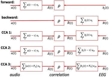
Auditory processing involves response latencies that are not perfectly known, and the convolutional transforms produced by CCA also contribute delays. In order to compensate for eventual differences in
Fig. 1. Overview of the models tested. In the forward model, the audio en-velope is transformed and compared with the EEG. In the backward model, the EEG is transformed and compared with the audio envelope. In CCA model
1, a FIRfilter is applied to the audio envelope and a spatialfilter to the EEG. In
CCA model 2, the spatialfilter is replaced by a multichannel FIRfilter. In CCA
model 3, FIR filters are implemented using a bank of filters Fk instead
of delays.
temporal alignment between stimulus and EEG, the entire process (model parameter estimation and correlation evaluation) is repeated for various
time shifts L of the audio relative to the EEG. The optimal shift is
determined from the peak of the correlation as a function of shift (see
Figs. 1–3). This ensures an optimal temporal alignment for every model.
This overall time shiftLis distinct from thefilter time lagsτthat appear in
some of the models (e.g. Eqs.(4) and (5)).
The decision to introduce a global time shiftLdistinct fromτwas
motivated by the desire to capture the effect of audio-to-EEG latency (fit
byL) separately from that of spectral mismatch (fit by coefficients of
aðtτÞorbðtτÞ,τ¼1…T). The alternative of a wider range ofτto
absorb latency would have entailed a larger number of parameters, and
made it harder to make a fair comparison with models that don't involveτ
(e.g. Eq.(4)). Introducing the parameterLallows each model to operate
in optimal conditions.
Models are also evaluated by designing aclassifierfor a simple
match-vs-mismatch classification task that involves deciding which of two
segments of audio gave rise to a particular segment of EEG data of
durationD. Segment duration is varied as a parameter, shorter durations
being harder to classify because they contain less discriminative infor-mation. Again, cross-validation is used to control for overfitting: the classifier is trained on a subset of the data, and the classification score
measured on unseen data. The classifier is trained and tested using the
time shiftLthat maximized correlation.
Evaluation data
The algorithms are evaluated using a database of EEG responses to
natural speech reported in a previous study (Di Liberto et al., 2015). Full
details of the stimulus and recording conditions are given in that refer-ence. In brief, EEG data were recorded from 8 subjects using a 128-channel Biosemi system with standard electrode layout, at 512 Hz sampling rate (data from 2 additional subjects recorded with a 160-channel system were not used). Each subject listened to 32 speech excerpts, each of duration approximately 155s from an audio book pre-sented diotically via headphones, for a total of approximately 1.4 h. The EEG data were downsampled to 64 Hz and detrended by subtracting a
10th-order polynomialfit weighted to exclude outliers using a robust
detrending routine (de Cheveigne and Arzounian, 2018). The STAR
al-gorithm (de Cheveigne, 2016) was used to suppress channel-specific
noise, and the data were convolved with a boxcar window of duration 20 ms to suppress 50 Hz and harmonics. The data were then high-pass filtered with a Butterworthfilter of order 2 and cutoff 0.1 Hz and rere-ferenced to the mean over channels. To calculate the stimulus' temporal envelope, the stimulus (sampled at 44,100 Hz) was squared, smoothed by convolution with a square window of width 15.6 ms (1/64 Hz), down-sampled to 64 Hz, and then raised to the power 1/3.
Models tested
To allow comparisons, we implemented backward and forward
models, and three versions of the CCA model as schematized inFig. 1.
In thebackward modelthe stimulus representationaðtÞis inferred
or“reconstructed”as a transformbðtÞof the EEG, for example a spatial filter:
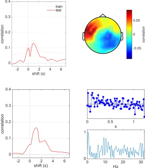
Fig. 2.Backward model. Left: correlation score between the
speech temporal envelope and the best linear combination of EEG, as a function of the overall temporal shiftL of the stimulus relative to the EEG, for one subject (EL). A positive value of the abscissa means that the envelope has been delayed relative to the EEG. Dotted line is measured on the training set, full line on the test set. Right: spatial topography of the correlation between EEG and envelope at the optimal shift.
Fig. 3.Forward model. Left: cross-validated correlation
score between the FIR-filtered stimulus temporal envelope and the best EEG channel as a function of the overall tem-poral shiftL of the stimulus relative to the EEG, for one subject (EL). Right: impulse response (top) and correspond-ing amplitude transfer function (bottom).
bðtÞ ¼X j bjðtþLÞuj; (8) or spatiotemporalfilter: bðtÞ ¼X j X τ bjτðtτþLÞuj; (9)
where the weightsujare calculated as the cross-correlation between the
audio and time-lagged EEG. This model was simulated based on Eq.(8)
(spatialfilter). The 128 EEG channels werefirst submitted to PCA and the
first 80 PCs retained, so the model had 80 parameters. The overall time
shiftLwas varied over a range from 3 toþ7 s, tofind the highest
correlation coefficient betweenaðtÞandbðtÞ. A variant of the model was
simulated based on Eq.(8)(spatiotemporal filter) with 17 time lags,
again with PCA to reduce the number of parameters to 80 (see Results).
In theforward modelthe response of a brain signal channelbjðtÞis
predicted from a transformaðtÞof the stimulus, for example a weighted
sum of time-lagged stimulus envelope samples (FIRfilter):
aðtÞ ¼X
τ aðtτþLÞvτ;
(10)
where the time shift L absorbs any temporal misalignment between
stimulus and EEG. To give this model the best chances to succeed, the prediction was applied to the optimal linear combination of channels found by the backward model, rather than to a particular brain signal
channel. The model was applied with 80 values of the delayτ(spanning
0–1.25 s), so this model too has 80 parameters.
InCCA model 1, both the stimulus and the EEG are transformed
ac-cording to: bðtÞ ¼X k bðtÞuk; aðtÞ ¼ X τ aðtτþLÞvτ; (11)
where the shiftLis varied to absorb any mismatch in response or
pro-cessing latency. CCA was applied to a set of 40 time lagged envelope signals and a set of 40 principal components of the EEG, producing 40 canonical correlate pairs. This model too has 80 parameters.
InCCA model 2, time lags are applied also to the EEG channels:
bðtÞ ¼X k X τ bðtτÞukτ; aðtÞ ¼ X τ aðtτþLÞvτ: (12)
The EEG was submitted to PCA and thefirst 60 PCs were selected and
submitted to 10 time lags. The compound matrix (600 channels) was submitted to PCA and 40 PCs retained, while the stimulus envelope was split into 40 time-lagged versions. This model too has 80 parameters. In a
variant of this model (model 2þ), 80 PCs were retained for both EEG and
audio, so the model had 160 parameters.
InCCA model 3, time lags are replaced by afilter bank, motivated as
follows. The stimulus envelope and EEG both include long-termfl
uctu-ations on the order of seconds. For example, these could reflect slow patterns shared by stimulus and response (e.g. phrase or semantic structure), or else slow artifacts that need to be removed. To resolve them
requiresfilters with a long impulse response which, if implemented as a
FIR, would require a filter of high order and thus many parameters
leading to overfitting. For example, at 64 Hz sampling rate a two-second impulse response requires 128 taps, which applied separately to 50 EEG PCs (multichannel FIR) involves 6400 parameters. To address this issue,
one can use a set offilterbank output channels as a“basis”for the space of
filters, instead of time lags. For aT-channelfilterbank the number of
parameters is the same as forT time lags, but thefilter subspace spanned
is different. With a logarithmic or waveletfilterbank the basis can include
both narrowfilters with long impulse response, and widerfilters with
shorter impulse response. CCA model 3 was tested with a dyadic bank of
FIR bandpassfilters with characteristics (center frequency, bandwidth,
duration of impulse response) approximately uniformly distributed on a
logarithmic scale. There was a total of 21 channels with impulse response
durations ranging from 2 to 128 samples (2 s). Thefilterbank was applied
to the stimulus envelope, yielding 21filtered signals, and also to the EEG
represented by 60 PCs, yielding 1260filtered signals that were submitted
to another PCA from which 139 PCs were retained. These two data sets (21 and 139 channels respectively) were then processed by CCA. Like the
previous model (CCA model 2þ), this model has 160 parameters. The
numbers chosen for this and previous models are largely arbitrary, the aim being to put the models in a range where they perform reasonably well, and allow comparisons between models with the same number of parameters.
Match-vs-mismatch classification was performed using Linear
Discriminant Analysis (LDA) trained on the model correlation scores. The ability of each model to identify matching EEG and audio segments was
assessed using leave-one-out cross-validation. The classifier was trained
on all time segments from 31 of the 32 trials and tested on all segments in
the remaining trial. To examine classification accuracy as a function of
test data duration, we performed the classification with time segments of
duration 1–64 s. This provided between 4960 (for 1 s segments) and 64 (for 60 s segments) non-overlapping tokens for classification.
Results
This section compares the performance of the different approaches
described in Sect.2, and investigates how the multiple canonical
corre-late pairs revealed by CCA can be used for classification.
Comparison between models
In the paragraphs to follow, we compare forward and backward models with CCA, using correlation as a performance metric.
Backward model
Fig. 2(left, full line) shows the correlation coefficient between the
spatially filtered EEG and the speech temporal envelope, with
cross-validation, as a function of the shiftL, for one subject. The correlation
coefficient is large for values ofLnear zero and falls for larger positive or
negative values. The dotted line shows the coefficient without
cross-validation. Plots in all otherfigures represent cross-validated
correla-tion coefficients.Fig. 2(right) shows the spatial distribution over the
scalp of the correlation coefficient between stimulus envelope and
indi-vidual EEG channels. Coefficients for individual channels approach
~0.09, whereas the linear combination (Eq.(8)) yields a score of ~0.13,
reflecting the benefit of the spatialfiltering.
Other studies, e.g. (O'Sullivan et al., 2014), used a model similar to
Eq. (9) in which the stimulus is modeled as a weighted sum of
time-lagged EEG channels. We simulated such a model using a set of 17
time lags (spanning 0–250 ms) as described in the Methods, using PCA to
reduce the number of parameters to 80 as in the previous model. The peak score with this version was 0.17, vs 0.13 with the previous
non--lagged model (Eq.(8)), suggesting a benefit of reconstruction based on
spatio-spectralfiltering over purely spatialfiltering.
Forward model
Fig. 3(left) shows the correlation coefficient between the filtered
stimulus envelopeajðtÞand the best EEG channel (the channel that yields
the highest correlation score). As for the backward model, the correlation
coefficient peaks for small values ofLand falls for larger positive or
negative values.Fig. 3 (right) shows the impulse response (top) and
transfer function (bottom) of the FIRfilter for the best shift. The transfer
function peaks near 1 Hz, suggesting that correlation is better at the lower end of the frequency range.
The backward model was calculated from 80 PCs, while the forward model involved 80 time lags, so the degrees of freedom were the same for
both. The second model applies an FIRfilter applied to the stimulus
envelope to predict an EEG channel, whereas the second applies spatial –
filter applied to the EEG data to infer the stimulus envelope. Since these
filtering operations address different sources of noise, it is worth
considering combining the two. The next sections explore how to do so in a systematic way using CCA.
CCA model 1
Thisfirst model is designed to be most comparable to the forward and
backward model. Subsequent models take advantage of theflexibility of
CCA to introduce a series of improvements.Fig. 4(first panel, red) shows
the correlation coefficients for thefirst canonical correlate (CC) pair as a
function of time shift. Values are comparable to the forward and
back-ward models, but CCA producesmultipleCCs beyond thefirst (thin lines),
several of which seem to show elevated correlation scores for a limited
range of shiftsL.
CCA model 2
CCA model 2 allows time shifts for the EEG channels (Eq.(12)).Fig. 4
(second panel, red) shows the correlation coefficients for thefirst
ca-nonical correlate (CC) pair as a function of temporal alignment between stimulus and EEG. Values are higher than for the previous model,
pre-sumably as a result of the moreflexible spatio-spectralfilter. It is likely
that the multichannel FIRfilter adapts the spectral content of the EEG
signals to that of the stimulus envelope. Thin lines show correlation
co-efficients for subsequent CC pairs.
Fig. 4(third panel, red) shows similar results assuming 80 time lagged stimulus envelope signals (instead of 40), and 80 PCs of time-lagged EEG signals (instead of 40) for a total of 160 parameters. Values are higher than for the smaller model, indicating that the more complex model gives
a betterfit to the data. This outcome was not a forgone conclusion, as the
more complex model could instead have led to overfitting and thus a
lower score with cross-validation. The larger correlation coefficients
likely reflect the ability of higher-order FIRs to capture and resolve fea-tures on a longer time scale.
CCA model 3
Fig. 4(fourth panel, red) shows the correlation coefficient for thefirst
CC pair as a function of time shift. The correlation coefficient approaches
0.4 at the best shift, indicating that CCA has discovered a transform of the stimulus that is highly predictive of a component extracted from the EEG
by applying a spatio-spectralfilter. In addition to this CC pair, there are
additional well-correlated pairs, further discussed in the next Section. The correlation coefficients for all subjects for these different models
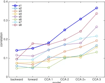
are summarized inFig. 5(the previous subject is the thick blue line). The
values differ greatly between subjects, but the trends are overall similar. A Wilcoxon rank-sum test indicates that CCA conditions yield
significantly larger scores than either forward or backward models
(p<0.002, not corrected for multiple tests) and that CCA model 3 yields
larger scores than any other model (p<0.002, not corrected).
Exploiting multiple canonical components
A useful feature of CCA solutions is that there aremultipleCCs with
elevated correlation scores (Fig. 4). Each CC corresponds to a particular
FIR-filtered stimulus-envelope signal, orthogonal to those of the other
CCs, and that differs from the others in spectral magnitude and/or phase. In this sense, CCA performs a decomposition of the stimulus envelope in
the modulation spectrum domain (Dau et al., 1997). Each CC is also
associated with a spatial- or spatio-spectrally filtered EEG signal
orthogonal to those of the other components, that differs from the others in spatial pattern and/or spectral magnitude and/or phase. CCA thus also decomposes the brain response into uncorrelated components, each mapped to a component of the stimulus envelope.
Fig. 6(top) shows the magnitude transfer functions of the FIRfilters
corresponding to thefirst 12 CCs of model 3 for subject EL. For most CCs
the transfer function peaks in a particular spectral region, although the peak-to-skirt ratio is usually modest (roughly 4:1 in magnitude, 16:1 in
Fig. 4.CCA models. See text for a description of each model.
Each plot shows the correlation coefficient between canoni-cal correlate pairs as a function of the temporal shift of the stimulus relative to the EEG, with cross-validation, for one subject (EL). One signal of each pair is derived byfiltering the stimulus envelope with a FIRfilter, and the other from the EEG byfiltering with a spatial (leftmost) or multichannel FIRfilter. The red line in each plot is thefirst (“best”) pair, other lines are for subsequent CC pairs.
Fig. 5.Best correlation scores for each subject as a function of the model. The
thick blue line is the subject (EL) used for the comparison in Figs. 1–3
andFig. 5.
power density). Each CC appears to cover a different spectral region but with considerable overlap between CCs. In this example, the transfer functions are peaked, and the peak frequencies roughly follow the order of the components, suggesting greater correlation values for lower fre-quencies, although the pattern is not perfect.
Fig. 6(bottom) shows the corresponding EEG topographies, calcu-lated as the cross-correlation between the FIR-filtered envelope signal and the raw EEG channels (the polarity of each component is arbitrary). The topography gives a rough indication of the spatial substrate of the EEG component of the CC pair. Whereas the time-courses of activation are mutually orthogonal, there is no such constraint on the associated topographies, and indeed several seem quite similar. The patterns for weaker components tend to be noisy (note the different color scales for each CC).
As argued elsewhere (de Cheveigne and Parra, 2014) it is not possible
to establish a one-to-one correspondence between components and
spe-cific sources within the brain. Component waveforms are mutually
un-correlated, whereas brain activity implicated in perceptual processing is likely to be correlated between sources. Even if the sources were un-correlated, the source-to-component mixing matrix might not be diago-nal. What can be said is that the components obtained from the analysis
span a subspace of the EEG data containing the stimulus-related behavior. From a neuroscience perspective, the most interesting impli-cation is that there are multiple processes, and that they cannot be sub-sumed by a single TRF model. CCA may be a useful tool to unravel them.
Classification
Another yardstick to measure a stimulus-response model is its per-formance in a classification task. Here we consider the task of deciding,
given segments of stimulus and EEG of durationT, whether the EEG was
in response to that stimulus or to an unrelated stimulus, using correlation scores as a feature as in prior studies. Classification involves determining
whether a sample belongs to either of two distributions (Duda et al.,
2012), in this case those of correlation scores for matched and
mis-matched segments respectively. Assuming Gaussian distributions with
equal variance, the performance of a one dimensional linear classifier
depends on the ratio of between-class to within-class variance, that can
be quantified by the d' metric (distance between means divided by
standard deviation). In the case of the forward and backward models, there is only one discriminant dimension, in the case of CCA there may be multiple discriminant dimensions.
Fig. 6.CCA model 3. Top: amplitude transfer functions of
thefirst 12 CCA-derived FIRfilters applied to the stimulus envelope normalized to a peak value of 1, for one subject (EL). Bottom: corresponding topographies. The value at each point of the topography is the normalized cross-correlation coefficient between the EEG component waveform and the EEG channel waveform. Signs are arbitrary. Note that the color scale differs between components, reflecting the lower SNR of higher-order components.
Fig. 7(a) shows thed' scores for thefirst 6 CC pairs from CCA model 3, as a function of the size of the data segment over which the correlation
between pairs is calculated. Thed' values increase as the data segment
becomes longer (as there is more information and estimates are more
stable), and are greater for thefirst than for subsequent CC pairs. Values
for thefirst few pairs are also greater than for the forward and backward
models (Fig. 7(c)). CC pairs that lead to large correlation scores tend to
show large values ofd' (Fig. 7(b)), although the ratio betweend' and
correlation tends to be smaller for pairs for which the component waveforms are dominated by low frequencies (coded as blue) rather than
higher frequencies (coded as red). Frequency content is quantified here
by calculating the centroid of the power spectrum of the component waveform.
Rather than using individual CCs, correlation values can be combined over CC pairs using multivariate Linear Discriminant Analysis (LDA), as
illustrated inFig. 7(d) (thick blue line) for the principal discriminant
dimension. As expected, combining features from multiple CC pairs leads
to better discrimination than the best CCFig. 7(d) (thin blue line), itself
better than either the forward and backward models (red and orange
lines). The dashed line in Fig. 7(d) shows the 95th percentile of the
classification score attained for 1000 random permutations of the class
labels. We chose a simple linear classifier for simplicity and ease of exposition. A companion paper describes results with more sophisticated
classifiers and classification strategies.
The match-vs-mismatch task, also chosen for simplicity of exposition, differs from the cocktail-party task considered by other studies (which of two concurrent streams is attended by the listener), although it captures
the main aspects of that task. Here, the classifiers were trained over a
relatively large dataset (>one hour) and tested on segments of new data,
analogous to what might occur in a practical system designed to control a device (see paragraph Relevance for Applications of the next Section).
Note that the durations indicated inFig. 7(d) do not take into account the
impulse responses offilters implied in certain models, so the amount of
data involved in each case is slightly longer. In other words, the nominal durations may not faithfully characterize the ability of a classifier to track rapid changes in attention. The issue of classification latency is complex (it depends on the time scales of attention-dependent features as well as noise) and is explored in a companion paper.
Discussion
This study used CCA to reveal a subspace of cortical activity well correlated with ongoing auditory stimulation (speech). CCA yielded more accurate predictions (larger correlation values) than simpler for-ward and backfor-ward models on the same data, and allowed better
classification. The presence of multiple CC pairs with different spatial
signatures suggests that the analysis taps a complex cortical process involving multiple sources. The multiple discriminative dimensions support a wider range of classification schemes, and relatively good
classification scores were obtained with short data segments, which is a
step towards the goal of controlling an external device (for example a hearing aid) on the basis of cortical signals measured by EEG.
This study builds upon a growing body of work exploring stimulus-response relations using system-identification techniques and decoding (Lalor et al., 2009; Lalor and Foxe, 2010; Power et al., 2011, 2012; Pasley et al., 2012; Ding and Simon, 2012; Brandmeyer et al., 2013; Ding and Simon, 2013; Ding et al., 2014; O'Sullivan et al., 2014; Koskinen and Sepp€a, 2014; Treder et al., 2014; Di Liberto et al., 2015; Mirkovic et al., 2015; Baltzell et al., 2016; Crosse et al., 2016; Ki et al., 2016; O'Sullivan et al., 2017; Biesmans et al., 2017; Fiedler et al., 2017; Khalighinejad et al., 2017; Fuglsang et al., 2017). Invasive measurements such as ECoG (Mesgarani and Chang, 2012; Tankus et al., 2012; Zion Golumbic et al., 2013; Chan et al., 2014; Martin et al., 2014; Leonard and Chang, 2014; Mesgarani et al., 2014; Lotte et al., 2015; Martin et al., 2015; Herff et al., 2015; Rao et al., 2017) support reconstruction of detailed spec-trotemporal or symbolic representations of the stimulus, while EEG and MEG have been related to coarser representations such as the stimulus waveform envelope, as used here. Whereas ECoG samples mass electric
fields relatively close to their source, the quality of EEG and MEG signals
is degraded by source-to-sensor mixing and additional sources of noise. Methods such as CCA can contribute to improve the quality of these signals.
A complex stimulus-response relationship for continuous speech
Each CC pair is characterized by afilterapplied to the speech
enve-lope. Each suchfiltered envelope waveform is orthogonal to the others,
and together they form an empirical decomposition that splits the stim-ulus envelope into components spectrally distinct in amplitude and/or
phase (Fig. 6, top). This is analogous to decomposition over amodulation
filterbank, a hypothesized component of perceptual processing (Dau et al.,
1997; Ewert and Dau, 2000; Lorenzi et al., 2001; Singh and Theunissen, 2003; Joris et al., 2004; Ghitza, 2011; McDermott and Simoncelli, 2011; Giraud and Poeppel, 2012; Wang et al., 2012; Xiang et al., 2013) that has also been proposed as relevant for processing temporally modulated
sounds such as speech (Elhilali et al., 2003; Sukittanon et al., 2004;
Hermansky, 2010; Nemala et al., 2013). Early studies applied a bandpass filter to EEG data to optimize SNR, e.g. 2–35 Hz (Lalor and Foxe, 2010) or
2–8 Hz (O'Sullivan et al., 2014).Koskinen and Sepp€a (2014)applied a
logarithmic filterbank (wavelet analysis) to MEG data, obtaining
Fig. 7. Match-vs-mismatch classification. (a)d' metric for the correlations of thefirst 6 CC pairs from CCA model 3, calculated over intervals of various durations.
(b) Scatterplot ofd' values (for an interval of 64s) versus correlation for all subjects and CC pairs up to rank 12. The color indicates the spectral centroid (in Hz) of
the audio envelope-derived component of the pair. (c)d' metric for the forward and backward models, thefirst CC pair of CCA model 3, and the joint multivariate
LDA model (thick blue line). (d) Percentage correct scores for a linear discriminant classifier for the same models as in (c). The dashed line inFig. 7(d) shows the
95th percentile of the classification score attained for 1000 random permutations of the class labels.
relatively high correlation values within each band, particularly for the
lowest frequency bands.Crosse et al. (2015)performed a similar analysis
on EEG data using a linearfilterbank (bandwidth 2 Hz). Compared to a
filterbank, the empirical decomposition provided by CCA allowsfilter parameters to be directly optimized in both amplitude and phase (at the risk of overfitting, see paragraph Caveats).
Each CC is also characterized by aspatiotemporalfilterapplied to the
EEG data. Eachfiltered EEG waveform is orthogonal to the others, and
together they form a decomposition of the cortical activity into compo-nents that are spectrally and/or spatially distinct. Evidence has been found for spatially differentiated responses as a function of selective
attention (Power et al., 2012; O'Sullivan et al., 2014; Fuglsang et al.,
2017), linguistic competence (Brandmeyer et al., 2013), intelligibility
(Tiitinen et al., 2012), phonemic feature (Khalighinejad et al., 2017), or
modulation frequency band (Wang et al., 2012; Koskinen and Sepp€a,
2014). The general pattern suggests an early response to acoustic features
from primary regions, and later responses to higher-order features (e.g.
phonetic) from multiple secondary cortical regions (Norman-Haignere
et al., 2015). CCA captures this spatially distributed and
temporally-staggered activity, although, as mentioned earlier, there is not a one-to-one correspondence between components and neural sources.
Canonical correlation analysis
CCA is a powerful tool tofind linear transforms to apply to time series
of brain data (Correa et al., 2010a; D€ahne et al., 2015). Like PCA it
produces component time series that are mutually decorrelated, but whereas PCA maximizes variance, CCA is designed to maximize corre-lation with a second set of time series. CCA is symmetrical with respect to the datasets, and thus a similar transform is found for the second set that
maximizes correlation with the first. Components come by pairs
(ca-nonical correlates), thefirst pair consisting of the linear combinations of
either data set with the highest possible correlation between them. CCA is intended for multichannel data, but can be applied to single channel data by augmenting them with time-lags. The solution (linear
combination of time-lagged data) is then aFIRfilter, the effect of which is
to equalize the spectrum of the time series so as to maximize its corre-lation with the other dataset. Applying time lags to multichannel data
results in multichannel FIRfiltersthat exploit both spectral and spatial
structure. The time lags can also be replaced by other convolutional
transforms (such as the logarithmicfilterbank we used here). Finally,
applying nonlinear transforms to the data before CCA allows it to capture non-linear relations between data sets, that can also be found using deep
learning techniques (Bießmann et al., 2009; Andrew et al., 2013; D€ahne
et al., 2015; Wang et al., 2015; Tang et al., 2017). CCA is aflexible tool to discover complex convolutional and non-linear relations between sets,
but thisflexibility is of course offset by the risk of overfitting entailed by
the many parameters involved (see paragraph Caveats).
In a recent study CCA was used to characterize auditory and
audio-visual EEG responses (Dmochowski et al., 2017). They applied
time-lags to the stimulus representation but not both stimulus and EEG, and they did not consider a convolutional basis other than time lags, both of which provided significant improvements in our study. CCA was used byBiesmans et al. (2017)to combine information across channels of an
auditoryfilterbank to maximize correlation with EEG, and byKoskinen
and Sepp€a (2014) to maximize trial-to-trial reproducibility before relating stimuli to responses. CCA is one example of a wider class of methods that apply linear transforms to EEG to isolate components
correlated between datasets (Bießmann et al., 2009; Dmochowski et al.,
2012, 2015; Lankinen et al., 2014; Sturm et al., 2015; Biesmans et al.,
2017) or between modalities (Correa et al., 2010b; Sui et al., 2013).
Caveats and cautions
As other data-driven analysis techniques, CCA is prone to overfitting
and circularity (Kriegeskorte et al., 2009). The risk is aggravated because
of the many parameters, particularly if multiple transforms of the data (convolutional and non-linear) are included. Overfitting may be detected and to some degree remediated using standard cross-validation and
surrogate data techniques, and the tendency to overfit limited by
dimensionality reduction, regularization, or prior constraints (Jiang and
Guo, 2007; Lahti et al., 2009; Andrew et al., 2013). While dimensionality reduction and regularization are closely related, we prefer the former as it allows dimensionality to be reduced based on criteria other than that optimized by CCA (e.g. spectral content, or repeatability), and competing models can be put on a similar footing by giving them the same number of free parameters.
CCA, based on least-squares minimization, is prone to large-amplitude outliers and glitches that may dominate the solution. It may also pick up artifacts that happen to be correlated between data sets,
such as power line interference, linear trends, or filtering transients.
Introducing time lags (orfilters) allows CCA to synthesizefilters that
isolate particular frequency regions, leading to higher correlation scores (compare CCA model 2 and 3 to CCA model 1). However, higher correlation might also arise merely from the greater serial correlation
introduced by lowpass or narrowbandfiltering, that reduces the degrees
of freedom within the data and thus exacerbates overfitting. Indeed,
we observed that, for a given value of correlation, discriminability (d')
tends to be lower for components dominated by lower frequencies (Fig. 7(b)).
Fig. 7(d) reports classification scores for data segments as short as 1 s,
but it should be noted that these nominal durations donotinclude the
length of the FIR filters. This should be taken into account when
comparing models, or judging the ability of an algorithm to track fast changes in an application (see next section).
Relevance for applications
A motivation for this study was to develop a method to steer an auditory assistive device (e.g. hearing aid) using brain signals. Several studies have shown that it is possible to determine which sound source
among several is the focus of attention using EEG (Power et al., 2012;
O'Sullivan et al., 2014; Mirkovic et al., 2015; Fuglsang et al., 2017; Ki et al., 2016; Biesmans et al., 2017). Good performance has been reported for stimulus-response data of long duration (e.g. 30 or 60 s) for some subjects, but accuracy falls short of what would be needed for real-time control in a usable device. For example, a 95% accuracy (as reported byBiesmans et al. (2017)for their best subject at 30 s duration) would amount to one error in every 20 decisions. An error rate such as this is likely to be frustrating for a user, and having to wait tens of seconds for a decision is also not acceptable.
CCA brings our goal closer in at least three ways. The first is by
allowing the representations of both stimulus and response to be
opti-mized jointly, leading to higher correlation scores (Fig. 5) and better
classification (Fig. 7). The second is by providingmultiplediscriminant
measures that support multivariate classification as illustrated here with
a simple multivariate LDA classifier (Fig. 7(d)). The third is by providing
aflexible framework that can harness additional streams of information
(for example non-linear transforms of the data). The best scores reported
here (Fig. 7) still fall short of what is needed for a useful device, but the
CCA methodology opens many routes that may lead to better perfor-mance. In our opinion the value of CCA lies less in the scores reported here, however encouraging, as in the potential it offers for further development. A companion paper describes results with more
sophisti-cated classifiers based on CCA.
The computational costs associated with CCA are mild. The solution requires eigendecomposition of a covariance matrix that can be
calcu-lated incrementally and updated in real time, and efficient standard
methods are available for eigendecomposition. Once the solution has been derived, processing amounts merely to application of a
multi-channel FIR (Eqs.(4) and (5)).
Conclusion
CCA strips the brain response of variance unrelated to the stimulus, and the stimulus of variance that does not affect the brain response, and thus improves our observation of the relation between stimulus and response. The best performing CCA model produced multiple component
pairs, each consisting of a FIRfilter applied to the stimulus waveform,
and a multichannel FIRfilter (spatiotemporalfilter) applied to the EEG
signal. The spatial signatures of thesefilters were diverse, suggesting that
the analysis is sensitive to multiple neural sources, although there is no simple mapping of components to sources. Each pair was also associated
with a different FIRfilter applied to the stimulus envelope, indicating
sensitivity to different rates of change. Signal components isolated by
CCA supported effective classification, in particular thanks to the fact
that multiple discriminative components are available, bringing closer the perspective of a cognitively-controlled device based on recording of attention-sensitive correlates of auditory stimulation. CCA is of great interest as a tool to explore the effectiveness of transforms (e.g. nonlinear or convolutional) applied to the data, to further our understanding of perceptual processes and increase the effectiveness of applications.
Acknowledgements
This work was supported by the EU H2020-ICT grant 644732 (COCOHA), and grants ANR-10-LABX-0087 IEC and ANR-10-IDEX-0001-02 PSL*, as well as a Ulysses grant (2015) from the French Ministry of Foreign Affairs and the Irish Research Council. It draws on work per-formed at the 2015 and 2016 Telluride Neuromorphic Engineering workshops. Giovanni Di Liberto was supported by an Irish Research Council (GOIPG/2013/1249) Postgraduate Scholarship.
References
Andrew, G., Arora, R., Bilmes, J., Livescu, K., 2013. Deep canonical correlation analysis. In: Proceedings of the 30th International Conference on Machine Learning (ICML-13), vol. 28, pp. 1247–1255.
Baltzell, L.S., Horton, C., Shen, Y., Richards, V.M., D'Zmura, M., Srinivasan, R., 2016. Attention selectively modulates cortical entrainment in different regions of the speech spectrum. Brain Res. 1644, 203–212.
Biesmans, W., Das, N., Francart, T., Bertrand, A., 2017. Auditory-inspired speech envelope extraction methods for improved EEG-based auditory attention detection in a cocktail party scenario. IEEE Trans. Neural Syst. Rehabil. Eng. 25, 402–412.
Bießmann, F., Meinecke, F.C., Gretton, A., Rauch, A., Rainer, G., Logothetis, N.K., Müller, K.R., 2009. Temporal kernel CCA and its application in multimodal neuronal data analysis. Mach. Learn. 79, 5–27.
Brandmeyer, A., Farquhar, J.D., McQueen, J.M., Desain, P.W., 2013. Decoding speech perception by native and non-native speakers using single-trial electrophysiological data. PLoS One 8.
Chan, A.M., Dykstra, A.R., Jayaram, V., Leonard, M.K., Travis, K.E., Gygi, B., Baker, J.M., Eskandar, E., Hochberg, L.R., Halgren, E., Cash, S.S., 2014. Speech-specific tuning of neurons in human superior temporal gyrus. Cerebr. Cortex 24, 2679–2693. Correa, N.M., Adali, T., Li, Y.O., Calhoun, V.D., 2010a. Canonical correlation analysis for
data fusion and group inferences. IEEE Signal Process. Mag. 39–50. July. Correa, N.M., Eichele, T., Adalı, T., Li, Y.O., Calhoun, V.D., 2010b. Multi-set canonical
correlation analysis for the fusion of concurrent single trial ERP and functional MRI. NeuroImage 50, 1438–1445.
Crosse, M.J., Butler, J.S., Lalor, E.C., 2015. Congruent visual speech enhances cortical entrainment to continuous auditory speech in noise-free conditions. J. Neurosci. 35, 14195–14204.
Crosse, M.J., Di Liberto, G.M., Bednar, A., Lalor, E.C., 2016. The multivariate temporal response function (mTRF) toolbox: a MATLAB toolbox for relating neural signals to continuous stimuli. Front. Hum. Neurosci. 10, 604.
D€ahne, S., Bießman, F., Samek, W., Haufe, S., Goltz, D., Gundlach, C., Villringer, A., Fazli, S., Müller, K.R., 2015. Multivariate machine learning methods for fusing functional multimodal neuroimaging data. Proc. IEEE 103, 1–22.
Dau, T., Kollmeier, B., Kohlrausch, A., 1997. Modeling auditory processing of amplitude modulation. I. Detection and masking with narrow-band carriers. J. Acoust. Soc. Am. 102, 2892–2905.
de Cheveigne, A., 2012. Quadratic component analysis. NeuroImage 59, 3838–3844. de Cheveigne, A., 2016. Sparse time artifact removal. J. Neurosci. Meth. 262, 14–20. de Cheveigne, A., Arzounian, D., 2018. Robust detrending, rereferencing, outlier
detection, and inpainting for multichannel data. NeuroImage 172, 903–912. de Cheveigne, A., Parra, L.C., 2014. Joint decorrelation, a versatile tool for multichannel
data analysis. NeuroImage 98, 487–505.
Di Liberto, G.M., O'Sullivan, J.A., Lalor, E.C., 2015. Low-frequency cortical entrainment to speech reflects phoneme-level processing. Curr. Biol. 25, 2457–2465.
Ding, N., Simon, J.Z., 2012. Neural coding of continuous speech in auditory cortex during monaural and dichotic listening. J. Neurophysiol. 107, 78–89.
Ding, N., Simon, J.Z., 2013. Adaptive temporal encoding leads to a background insensitive cortical representation of speech. J. Neurosci. 33, 5728–5735. Ding, N., Chatterjee, M., Simon, J.Z., 2014. Robust cortical entrainment to the speech
envelope relies on the spectro-temporalfine structure. NeuroImage 88, 41–46. Dmochowski, J.P., Greaves, A.S., Norcia, A.M., 2015. Maximally reliable spatialfiltering
of steady state visual evoked potentials. NeuroImage 109, 63–72. Dmochowski, J.P., Ki, J.J., DeGuzman, P., Sajda, P., Parra, L.C., 2017. Extracting
multidimensional stimulus-response correlations using hybrid encoding-decoding of neural activity. NeuroImage 1–13.
Dmochowski, J.P., Sajda, P., Dias, J., Parra, L.C., 2012. Correlated components of ongoing EEG point to emotionally laden attention a possible marker of engagement? Front. Hum. Neurosci. 6, 112.
Duda, R.O., Hart, P.E., Stork, D.G., 2012. Pattern Classification. John Wiley&Sons. Elhilali, M., Chi, T., Shamma, S.A., 2003. A spectro-temporal modulation index (STMI) for
assessment of speech intelligibility. Speech Commun. 41, 331–348.
Ewert, S.D., Dau, T., 2000. Characterizing frequency selectivity for envelopefluctuations. J. Acoust. Soc. Am. 108, 1181–1196.
Fiedler, L., W€ostmann, M., Graversen, C., Brandmeyer, A., Lunner, T., Obleser, J., 2017. Single-channel in-ear-EEG detects the focus of auditory attention to concurrent tone streams and mixed speech. J. Neural. Eng. 14, 036020.
Fuglsang, S.A., Dau, T., Hjortkjær, J., 2017. Noise-robust cortical tracking of attended speech in real-world acoustic scenes. NeuroImage 156, 435–444.
Ghitza, O., 2011. Linking speech perception and neurophysiology: speech decoding guided by cascaded oscillators locked to the input rhythm. Front. Psychol. 2, 1–13. Giraud, Al, Poeppel, D., 2012. Cortical oscillations and speech processing: emerging
computational principles and operations. Nat. Neurosci. 15, 511–517.
Herff, C., Heger, D., de Pesters, A., Telaar, D., Brunner, P., Schalk, G., Schultz, T., 2015. Brain-to-text: decoding spoken phrases from phone representations in the brain. Front. Neurosci. 9, 1–11.
Hermansky, H., 2010. History of modulation spectrum in ASR. In: 2010 IEEE International Conference on Acoustics, Speech and Signal Processing. IEEE, pp. 5458–5461.
Hotelling, H., 1936. Relations between two sets of variates. Biometrika 28, 321–377. Jiang, Y., Guo, P., 2007. Regularization versus dimension reduction, which is better? Adv.
Neural Networks 474–482. ISNN 2007.
Joris, P.X., Schreiner, C.E., Rees, a, 2004. Neural processing of amplitude-modulated sounds. Physiol. Rev. 84, 541–577.
Khalighinejad, B., Cruzatto da Silva, G., Mesgarani, N., 2017. Dynamic encoding of acoustic features in neural responses to continuous speech. J. Neurosci. 37, 2176–2185. Ki, J., Kelly, S., Parra, L.C., 2016. Attention strongly modulates reliability of neural
responses to naturalistic narrative stimuli. J. Neurosci. 36, 3092–3101.
Koskinen, M., Sepp€a, M., 2014. Uncovering cortical MEG responses to listened audiobook stories. NeuroImage 100, 263–270.
Kriegeskorte, N., Simmons, W.K., Bellgowan, P.S.F., Baker, C.I., 2009. Circular analysis in systems neuroscience: the dangers of double dipping. Nat. Neurosci. 12, 535–540. Lahti, L., Myllykangas, S., Knuutila, S., Kaski, S., 2009. Dependency detection with
similarity constraints. In: Machine Learning for Signal Processing XIX - Proceedings of the 2009 IEEE Signal Processing Society Workshop. MLSP, 2009.
Lalor, E.C., Power, A.J., Reilly, R.B., Foxe, J.J., 2009. Resolving precise temporal processing properties of the auditory system using continuous stimuli. J. Neurophysiol. 102, 349–359.
Lalor, E.C., Foxe, J.J., 2010. Neural responses to uninterrupted natural speech can be extracted with precise temporal resolution. Eur. J. Neurosci. 31, 189–193. Lankinen, K., Saari, J., Hari, R., Koskinen, M., 2014. Intersubject consistency of cortical
MEG signals during movie viewing. NeuroImage 92, 217–224. LeCun, Y., Bengio, Y., Hinton, G., 2015. Deep learning. Nature 521, 436–444. Leonard, M.K., Chang, E.F., 2014. Dynamic speech representations in the human temporal
lobe. Trends Cognit. Sci. 18, 472–479.
Lorenzi, C., Soares, C., Vonner, T., 2001. Second-order temporal modulation transfer functions. J. Acoust. Soc. Am. 110, 1030–1038.
Lotte, F., Brumberg, J.S., Brunner, P., Gunduz, A., Ritaccio, A.L., Guan, C., Schalk, G., 2015. Electrocorticographic representations of segmental features in continuous speech. Front. Hum. Neurosci. 9, 1–13.
Martin, S., Brunner, P., Holdgraf, C., Heinze, H.J., Crone, N.E., Rieger, J., Schalk, G., Knight, R.T., Pasley, B.N., 2014. Decoding spectrotemporal features of overt and covert speech from the human cortex. Front. Neuroeng. 7, 14.
Martin, S., Millan, JdR., Knight, R.T., Pasley, B.N., 2015. The use of intracranial recordings to decode human language: challenges and opportunities. Brain Lang. https://www.sciencedirect.com/science/article/pii/S0093934X15301243. McDermott, J.H., Simoncelli, E.P., 2011. Sound texture perception via statistics of the
auditory periphery: evidence from sound synthesis. Neuron 71, 926–940. Mesgarani, N., Chang, E.F., 2012. Selective cortical representation of attended speaker in
multi-talker speech perception. Nature 485, 233–236.
Mesgarani, N., Cheung, C., Johnson, K., Chang, E.F., Francisco, S., 2014. Phonetic feature encoding in human superior temporal gyrus. Science 343, 1006–1010.
Mirkovic, B., Debener, S., Jaeger, M., Vos, M.D., 2015. Decoding the attended speech stream with multi-channel EEG: implications for online, daily-life applications. J. Neural. Eng. 12, 046007.
Nemala, S.K., Patil, K., Elhilali, M., 2013. A multistream feature framework based on bandpass modulationfiltering for robust speech recognition. IEEE Trans. Audio Speech Lang. Process. 21, 416–426.
Norman-Haignere, S., Kanwisher, N.G., McDermott, J.H., 2015. Distinct cortical pathways for music and speech revealed by hypothesis-free voxel decomposition. Neuron 88, 1281–1296.
O'Sullivan, J.A., Power, A.J., Mesgarani, N., Rajaram, S., Foxe, J.J.,
Shinn-Cunningham, B.G., Slaney, M., Shamma, S.A., Lalor, E.C., 2014. Attentional selection in a cocktail party environment can Be decoded from single-trial EEG. Cerebr. Cortex 25, 1697–1706.
O'Sullivan, J., Chen, Z., Herrero, J., McKhann, G.M., Sheth, S.A., Mehta, A.D., Mesgarani, N., 2017. Neural decoding of attentional selection in multi-speaker environments without access to separated sources. J. Neural. Eng. 14, 1–14. Pasley, B.N., David, S.V., Mesgarani, N., Flinker, A., Shamma, S.A., Crone, N.E.,
Knight, R.T., Chang, E.F., 2012. Reconstructing speech from human auditory cortex. PLoS Biol. 10, e1001251.
Power, A.J., Foxe, J.J., Forde, E.J., Reilly, R.B., Lalor, E.C., 2012. At what time is the cocktail party? A late locus of selective attention to natural speech. Eur. J. Neurosci. 35, 1497–1503.
Power, A.J., Lalor, E.C., Reilly, R.B., 2011. Endogenous auditory spatial attention modulates obligatory sensory activity in auditory cortex. Cerebr. Cortex 21, 1223–1230.
Rao, V.R., Leonard, M.K., Kleen, J.K., Lucas, B.A., Mirro, E.A., Chang, E.F., 2017. Chronic ambulatory electrocorticography from human speech cortex. NeuroImage 153, 273–282.
Singh, N.C., Theunissen, F.E., 2003. Modulation spectra of natural sounds and ethological theories of auditory processing. J. Acoust. Soc. Am. 114, 3394–3411.
Sturm, I., D€ahne, S., Blankertz, B., Curio, G., 2015. Multi-variate EEG analysis as a novel tool to examine brain responses to naturalistic music stimuli. PLoS One 10, 1–30. Sui, J., Adalı, T., Yu, Q., Calhoun, V.D., 2013. A review of multivariate methods for
multimodal fusion of brain imaging data. J. Neurosci. Meth. 204, 68–81. Sukittanon, S., Atlas, L.E., Pitton, J.W., 2004. Modulation-scale analysis for content
identification. IEEE Trans. Signal Process. 52, 3023–3035.
Tang, Q., Wang, W., Livescu, K., 2017. Acoustic feature learning via deep variational canonical correlation analysis. ArXiv 1708, 04673v2.
Tankus, A., Fried, I., Shoham, S., 2012. Structured neuronal encoding and decoding of human speech features. Nat. Commun. 3, 1015.
Tiitinen, H., Miettinen, I., Alku, P., May, P.J.C., 2012. Transient and sustained cortical activity elicited by connected speech of varying intelligibility. BMC Neurosci. 13, 157. Treder, M.S., Purwins, H., Miklody, D., Sturm, I., Blankertz, B., 2014. Decoding auditory attention to instruments in polyphonic music using single-trial EEG classification. J. Neural. Eng. 11, 026009.
Wang, W., Livescu, K., Bilmes, Ja, 2015. Unsupervised learning of acoustic features via deep canonical correlation analysis. In: IEEE International Conference on Acoustics, Speech and Signal Processing (ICASSP), pp. 4590–4594.
Wang, Y., Ding, N., Ahmar, N., Xiang, J., Poeppel, D., Simon, J.Z., 2012. Sensitivity to temporal modulation rate and spectral bandwidth in the human auditory system: MEG evidence. J. Neurophysiol. 107, 2033–2041.
Woodman, G.F., 2010. A brief introduction to the use of event-related potentials in studies of perception and attention. Atten. Percept. Psychophys. 72, 2031–2046. Xiang, J., Poeppel, D., Simon, J.Z., 2013. Physiological evidence for auditory modulation
filterbanks: cortical responses to concurrent modulations. J. Acoust. Soc. Am. 133, EL7.
Zaidi, Q., Victor, J., McDermott, J., Geffen, M., Bensmaia, S., Cleland, T.A., 2013. Perceptual spaces: mathematical structures to neural mechanisms. J. Neurosci. 33, 17597–17602.
Zion Golumbic, E.M., Ding, N., Bickel, S., Lakatos, P., Schevon, C.A., McKhann, G.M., Goodman, R.R., Emerson, R., Mehta, A.D., Simon, J.Z., Poeppel, D., Schroeder, C.E., 2013. Mechanisms underlying selective neuronal tracking of attended speech at a “cocktail party”. Neuron 77, 980–991.