José-María Montero
Gema Fernández-Avilés
University of Castilla-La Mancha, E-45071 Toledo, SpainE-mails: Jose.mlorenzo@uclm.es and Gema.faviles@uclm.es
Keywords: Mixed Environmental Quality Index (MEQI), pollutant, hedonic house price model, area-to-point kriging
Mixed environmental quality
indexes for hedonic housing price
models: an alternative with
area-to-point kriging with external drift
(a) When environmental variables are included in hedonic house price models, the locations where a property trans-action has been taken place are more than those equipped with an environmental monitoring station. (b) When en-vironmental variables are numerous, an enen-vironmental quality index (EQI) is needed. The solution is to interpo-late (kriging) environmental variables and, subsequently, elaborate an EQI, because of the lower prediction variance. (c) Environmental informations can be both objective and subjective. The potential mismatch between the spatial support for both the objective informations and the sub-jective ones is solved by using a kriging strategy (area-to-point kriging) that forces scarce objective environmental informations to be coherent with dense subjective ones. These options for elaborating EQIs are compared in Ma-drid City (Spain).1. Introduction
It is well known that environmental pollution is one of the main components to take into account in housing pricing, overall in the case of weekend houses, holiday houses or vacation apartments. Consequently, it is reasonable to assume that air and noise pollutants enter into the utility function of potential house buy-ers (Anselin and Lozano-Gracia, 2008), and it is not surprising that hedonic house price models that incorporate environmental variables among the set of explana-tory variables are becoming more and more popular.
But the importance of environmental variables when estimating housing pric-es is not only an intuition. It has been checked empirically. This checking procpric-ess is not an obvious question since there does not exist an explicit market for air pol-lutants, noise, etc. There exist several methods to empirically estimate the value of the above-mentioned pollutants, such as contingent valuation, conjoint analysis, discrete choice models and hedonic specifications, but the most successful have been the last ones. In the context of the framework of hedonic price theory, the traditional approach to this problem has been to use the housing market to infer the implicit prices of these non-market goods (see Freeman III, 1993, for a compre-hensive review of property value models for measuring the value of environmen-tal amenities; Braden and Kolstad, 1991, is also a recommended reference). Under standard assumptions of perfect competition, information and mobility, and the maximization of well-behaved preferences, hedonic theory unambiguously
pre-dicts that the implicit price function relating housing prices of an environmen-tal amenity will be positive sloped, all else equal. A substantial body of research empirically confirms the hedonic theory and suggests that consumers are willing to pay for environmental goods such as air quality, absence of acoustic pollution, etc. In Smith and Kaoru, 1995, 50 studies undertaken between 1967 and 1988 were reviewed, and 37 of them were identified as dealing with big cities offering he-donic price function estimations including air pollution measures. In the two last decades, Smith and Huang, 1993, 1995, Kim et al., 2003, Anselin and Le Gallo, 2006, Anselin and Lozano-Gracia, 2008, among others, are good examples of the focus on hedonic property-value models for estimating the marginal willingness of people to pay for a reduction in the local concentration of specified air pollut-ants. Nevertheless, in Chay and Greenstone, 2005, and Bayer et al., 1996, it has been questioned the traditional approach to estimating the economic benefits of environmental variables (in particular, air quality), because the “true” relationship may be obscured in cross-sectional analysis by unobserved determinants of hous-ing prices that co-vary with the environmental variables and propose the random assignment of air quality across localities.
The problem that usually arises when environmental information is included in hedonic house price models is that price of houses can be easily obtained in the desired locations of the area under study. But, unfortunately, the number of environmental monitoring stations is certainly scarce due to both physical and economic constraints (in De Iaco et al., 2002, it is used an air pollution data set available at 30 locations in Milan district, in Anselin and Le Gallo, 2006, 27 stations are considered in four Californian counties, in Anselin and Lozano-Gracia, 2008, measurements come from 28 monitoring stations for a pollutant and from 12 for the other pollutant considered in their analysis, also in South California, and in De Iaco et al,. 2002, only seven stations are investigated in Kraków).
In the specialized literature, the usual solution to the abovementioned problem is to interpolate the environmental variables to obtain their interpolated values in the locations where house prices are available. Several interpolative alternatives have been considered in recent research and they use to provide different predic-tions when dealing with environmental variables (Wong et al., 2004): Thiessen pol-ygons, inverse distance methods, splines, and kriging and cokriging. But kriging (when dealing with one environmental variable) and cokriging procedures (when dealing with several ones) have important advantages (Anselin and Le Gallo, 2006). In the presence of a unique environmental variable, kriging considers its spatial de-pendence, what is crucial obtaining optimal predictions when dealing with geo-re-ferred data. In a multivariate approach, cokriging not only accounts for the spatial dependence of each variable but also for the inter-variable correlation.
However, usually these variables are measured at the same monitoring sta-tions, and in this so-called isotopic case, cokriging obtains a hardly noticeable ben-efit in relation to kriging. In fact, in the specific case of autokrigeability, cokriging reduces to kriging (Subramanyam and Pandalai,
2004).
Otherwise, not only valid variograms are needed to represent the structure of the spatial dependence of the variables of interest, but also valid cross-variograms. This is one of the mainrea-son (particularly in a space-time context) why most of researchers opt to gener-ate a single measure as a linear combination of this variables applying Principal Component Analysis (PCA) (Preisendorfer, 1998, and De Iaco et al., 2001, 2002, in the spatial context, and Statheropoulos et al., 1998, and Wakernagel, 1998, in the spatio-temporal modelling, are good classical references). Then, as a final step, a spatial interpolation is carried out to determine the level of contamination across the city in order to point out the so called ‘hot points’. But another different pos-sibility can be considered: the cokriged (kriged in the isotopic case) interpolation of the environmental variables in the non observed locations and the subsequent elaboration of the environmental index using the weights coming from PCA.
Hedonic house pricing strategies usually only include objective environmen-tal variables (measures provided by monitoring stations), but subjective variables (people’s perceptions) are also crucial when it comes to estimate the impact of pol-lution on housing prices. Therefore, mixed EQIs (MEQIs) should be preferred to EQIs. The problem that arises when dealing with MEQIs, apart from the support problem, is the coherence between both objective and subjective environmental information. As traditional kriging strategies do not take into account this coher-ence problem between de objective and subjective environmental information, in this article a version of universal kriging, area-to-point kriging with external drift (A2PKED), is proposed to use both kinds of information (coming from different sources) in a coherent way.
Summarizing, when including several environmental variables in a hedonic house price model, three possibilities can be considered: (i) interpolate (preferably cokriging) such variables and include all variables in the model; (ii) elaborate an environmental index and then interpolate it (preferably kriging); and (iii) inter-polate (preferably cokriging) the environmental variables considered and, subse-quently, elaborate an environmental index.
Option (i) is preferred when dealing with only one environmental variable. In the case that several variables are included in the analysis, option (ii) is the one cho-sen in the specialized literature on the topic, arguing that it is a way to transform a multivariate problem in a univariate one. The last statement being true, in our opin-ion, option (ii) is not the best path to go from multivariate to univariate study of the problem. Best option is (iii) because the variance of the prediction error is less-er than using (ii); in othless-er words, replacing the vector of contaminant values, at a given location and/or time, by a weighted linear combination, as referred in option (ii), is not quite optimal as shown in Myers, 1983. But, as subjective environmental information is crucial to estimate the impact of environment on housing prices, op-tion (iii) is extended by using an A2PKED strategy, so that objective and subjective information (coming from different sources) can be coherently combined.
Therefore, when the objective is the elaboration of a MEQI to be included as an explanatory variable in a hedonic housing price model, the suggestion we make is to interpolate directly the environmental objective variables where neces-sary, taking into account two crucial aspects: their spatial autocorrelation and the coherence with people’s perceptions on pollution. Then, the last step is the gen-eration of the index. Although it is true that there are a number of articles about
kriging models applied to the area of environmental pollution and analysis in the environmental quality index theory, there are no examples in the literature follow-ing the proposal we present.
After this introduction, Section 2 includes the main rudiments of A2PKED, and theoretically faces options (ii) and (iii) above mentioned in terms of prediction mean square error. In Section 3, the proposed alternatives are empirically com-pared with the traditional one using objective air pollution measures (first alterna-tive) and both objective and subjective values (second alternaalterna-tive) in Madrid City (Spain). Finally, some concluding remarks and future research lines are reported in Section 4.
2. Methods
2.1. A2PKED theory
Researching the environment of a particular city in a real case, it is impossible to get exhaustive (even complete) values of data at every desired point because of practical constraints. Thus, interpolation is important and crucial to graphing, analyzing and understanding the environmental results. Assuming the great im-portance of the particular spatial location when analyzing environmental quality, among all the existing interpolation methods, geostatistics uses kriging to take ac-count of spatial dependencies. Kriging is a univariate procedure which interpo-lates the values of the target random function at unobserved locations using the available observations of the same random function. This interpolation procedure – which is a minimum mean-squared-error method of spatial prediction – produc-es the bproduc-est linear unbiased predictor and usproduc-es the covariance or variogram func-tion (the spatial equivalent of the autocorrelafunc-tion funcfunc-tion in time series analysis) to account for the correlation structure in making interpolative predictions.
Kriging can be viewed as a strategy equivalent to time series, but in space. It is based on the idea of stochastic processes or random functions over space, taking into account the multidirectional feature of the space in a concrete instant of time. This approach applies to a wide range of phenomena, cf. Tzeng et al., 2005, Spence et al., 2007, Montero, Larraz, 2008, and implies dealing with an infinite family of ran-dom variables X(s) constructed at all points s in a region. The variables take differ-ent values depending on the location and the correlation structure, and each set of observed dataset is supposed to be a realization of the random function under study.
Observing the set of air quality monitoring sites as a group of points in a map, the pollution level measured at each site could be regarded as a realization of a spatial random function. As the monitoring sites only report these levels for s1,
s2, …, sn then interpolation is used to predict the pollution level for the locations
(more than n) where housing prices are disposable. In our case, Xh – the level of
pollutant h – are the random functions considered in the analysis, Xh(si) are the
random variables derived from that functions, and represent the level of hth
for pollutant h at the ith site. When obtaining a kriged prediction for the level of
pollutant h, the observed Xh(si)= xhi for i=1,2,..,n, are available at each air
monitor-ing sites, and the level for that pollutant at each location where housmonitor-ing prices are disposable, j, j∈{1,…,m}, is predicted as a weighted average of the level of pollut-ant obtained at sampled sites through the linear equation (1):
Xh j iXh i n i *( )s = ( )s =
∑
λ 1 1 (1)Depending on the nature of the particular random function we deal with, dif-ferent types of punctual kriging can be distinguished: simple kriging, ordinary kriging, and universal kriging. In this work, given the nature of the air pollution, the data are considered as a realization of a non-stationary random function X( )s
that can be decomposed as follows:
X( )s =μ
( )
s +R( )
s , s∈D (2)μ(s) being the drift, that describes the average of a pollutant over the studied area, and is typically specified by a linear combination of a number of covariates describing the pollution underlying factors; and R(s) representing a zero-mean RF that captures the spatial variation of the level of a particular pollutant unex-plained by the drift. In other R(s) can be seen as a factor driving the spatial varia-tion in the polluvaria-tion process.
Now consider the task of predicting the unknown value of a particular pol-lutant at s0 using the objective information coming from the monitoring stations
located in si, i=1, 2, …, n in the area under study, x(si) and the subjective
informa-tion corresponding to the areal (census tracks) averages, x(sk), k=1, 2, …, K over
the K areas in which the studied domain has been divided. The inclusion of these last values is extremely useful when the number of objective data is limited. Given the n values provided by the monitoring stations, and the K values corresponding to the areal data, the A2PKED prediction x*(s0) of an unknown pollutant value at
location s0 is obtained as:
x ix x i n i k A k K k * s s s 0 1 1
( )
=( )
+( )
= =∑
λ∑
λ (3)where λi are the A2PKED weights associated with the objective values of a
par-ticular pollutant, and λkA denotes the A2PKED weights assigned to the K
area-av-eraged subjective data.
In the framework of the A2PKED strategy, the classical kriging requirement of
E Xk*( )s Xk( )s
0 − 0 0
⎡
⎣⎢ ⎤⎦⎥= leads to the following conditions:
λi λ i n i m i k A k K k m k m x f x f f m = =
∑
( ) ( )
+∑
( ) ( )
=( )
1 1 0 s s s s s , ==0 1, , , M (4)1 The value of the prediction depends upon the weights λ
where fm(si) the (m+1)-th predictor value known at the location si and fm(sk) is the
area-average of predictor values associated with the areal support for subjective information sk.
As in other kriging strategies, x*(s0) is obtained by minimizing the
predic-tion error variance, V Xk*( )s Xk( )s
0 − 0 subject to the previous unbiasedness constraints. This is accomplished by introducing (M+1) Lagrange multipliers
αm
( )
s0 , m=0 1, , , M the resulting A2PKED system being obtained as:Σ Σ Σ Σ ss sA s As AA A s A F F F F 0 R R R R ′ ′ ′ ′ ⎛ ⎝ ⎜⎜ ⎜⎜ ⎜⎜ ⎜⎜ ⎜⎜ ⎞ ⎠ ⎟⎟⎟ ⎟⎟⎟⎟ ⎟⎟⎟ ⎟⎟⎟ ⎛ ⎝ ⎜⎜ ⎜⎜ ⎜⎜ ⎜⎜⎜ ⎞ ⎠ ⎟⎟⎟ ⎟⎟⎟ ⎟⎟⎟ ⎟⎟ = λ λ σ σ s s A 0 0 0 0 A α 00 0 fs ⎛ ⎝ ⎜⎜ ⎜⎜ ⎜⎜ ⎜⎜ ⎜⎜ ⎞ ⎠ ⎟⎟⎟ ⎟⎟⎟ ⎟⎟⎟ ⎟⎟⎟ (5) with F s s s s s=
( )
( )
( )
( )
⎛ ⎝ ⎜⎜ ⎜⎜ ⎜⎜ ⎜⎜ ⎜⎜ ⎞ ⎠ ⎟ f f f f M n M n 0 1 1 0 ⎟⎟⎟⎟ ⎟⎟⎟ ⎟⎟⎟ ⎟⎟ =( )
( )
( )
( )
⎛ ⎝ ⎜ F A A A A A f f f f M K M K 0 1 1 0 ⎜⎜⎜ ⎜⎜ ⎜⎜ ⎜⎜⎜ ⎞ ⎠ ⎟⎟⎟ ⎟⎟⎟ ⎟⎟⎟ ⎟⎟⎟ = ⎛ ⎝ ⎜⎜ ⎜⎜ ⎜⎜ ⎜⎜⎜ ⎞ ⎠ ⎟ α α α 1 0 0 M ⎟⎟⎟⎟ ⎟⎟⎟ ⎟⎟⎟⎟ =( )
( )
⎛ ⎝ ⎜⎜ ⎜⎜ ⎜⎜ ⎜⎜ ⎜⎜ ⎞ ⎠ ⎟⎟⎟ ⎟⎟ f s s s 0 0 0 0 f fM ⎟⎟⎟⎟ ⎟⎟⎟⎟ where ΣssR s s R i j C i j n=
{
( )
, , , =1 2, , ,}
denotes (nxn) matrix of co-variance values among two individual residual RVs R(si) R(sj)ΣsAR s A
R i k
C i n k K
=
{
(
,)
, =1 2, , , , =1 2, , ,}
is a (nxK) of cross-covariance val-ues between any pair of punctual residual RVs R(si) block residual variables(ar-eal average residuals) R(sk) ΣRAA=
{
CR(
s sk, k′)
, k k, ′ =1 2, , , K}
denotes thematrix of covariances between the mean values representing the considered ar-eas; Fs is a (nx(M+1)) matrix with
{
fm( )
si i=1 2, , , , n m=0 1, , , M}
FA is aKx M
(
+)
(
1 whose terms)
{
fm( )
Ak k=1 2, , , , K m=0 1, , , M}
the area-aver-aged covariates associated with the K areas included in the domain under study. The ((M+1)x(M+1)) of zeros is denoted 0. The terms of (n+1)σ
s0 are thecov-ariance values between the n punctual residuals RVs and the prediction point RV, i.e. σs0 s s
0 1 2
=
{
CR( )
i, , i= , , ,n}
and, similarly, the (Kx1) vectorσ
0A contains thecovariance values between the K areal residuals RVs and the prediction point RV, i.e. σA0 s s
0 1 2
=
{
CR(
k,)
, k= , , , K}
Finally, fs0 a ((M+1)x1) vector that denotes thecovariate values known at the prediction s0.
The A2PKED prediction in Equation 2 can be also derived as the sum of a drift obtained via GLS, and a residual obtained via Area-to-Point Simple Kriging (A2PSK) (Chilès and Delfiner, 1999). As a consequence of this, the A2PKED predic-tion error variance at the predicpredic-tion locapredic-tion can be written as:
ˆ ˆ ˆ ˆ σ2 σ σ σ 0 2 0 2 2 0 2 1 0 s s s
( )
=( )
+( )
=( )
− = Drift A PSK R i i λ nn i k A k K k m m m M C C f∑
( )
−∑
(
)
+∑
( )
= = s s, 0 s s, s 1 0 0 0 λ α (6)That is, the A2PKED prediction variance can be expressed as the sum of the A2PSK variance for the unknown residual r(s0) and the prediction variance for the
unknown drift s0.
Variograms are obtained following a two steps procedure. First, using the clas-sical variogram estimator based on the method-of-moments (Lark and Papritz, 2003), ballpark point estimates of the variograms are reached. Second, to ensure a permissible model, a theoretical variogram function (see, e.g. Emery, 2000, pp 93-104) is fitted to the sequence of average dissimilarities in keeping with the linear model of regionalization. GeoR, a package for geoestatistical data analysis using the R software, has been used to compute variograms, carry out the cross valida-tion procedure, and obtain kriging predicvalida-tions.
2.2. An alternative kriged procedure for making EQIs
Once the A2PKED rudiments have been briefly presented, the rest of the sec-tion is focused on why kriging the environmental variables and then elaborate an environmental index is a better option than the usual procedure in the litera-ture that consists of making an environmental index to be eventually interpolated (kriged). For theoretical purposes, we use cokriging terms, more general than krig-ing ones, but in practice the simplicity criterion leads us to use krigkrig-ing as cokrig-ing obtains a hardly noticeable benefit in relation to krigcokrig-ing in the isotopic case.
Let X1, X2, …, XH the level of h different pollutants, be intrinsic stationary
ran-dom functions of order zero, and consider an EQI given by
EQI i a Xh h k K i s s A X
( )
=( )
= ′ =∑
1 (7) where ′ =(
)
A a1, , aH and X′ =(
X1( )
si , , XK( )
si)
(8) The two options to linearly predict the value of EQI the unknown location are:(i) Elaborate a EQI using the environmental information provided by the moni-toring stations and then obtain the kriged predictions in locations (N) where housing prices have been observed, that is,
EQI j iEQI j m i *
( )
s =( )
s =∑
λ 1 j=1, …, N (9)(ii) Cokrige X1(s), …, XH(s) in locations where housing prices have been observed
EQI j j a Xk h a X s h H j k i h h i h i nj
( )
s =A X =( )
s =( )
= =∑
' * * 1 1 λ∑
∑
∑
= k K 1 (10)Following Myers, 1983, in general
Var EQI*
( )
s −EQI( )
s >Var EQI( )
s −EQI( )
s (11)that is, MSE is lesser when choosing option (ii) or, in other words, replacing the vector of contaminant values at a given location by a weighted linear com-bination and then kriging such a linear comcom-bination is not quite optimal.
3. Case study: Elaboration of an EQI for Madrid City (Spain)
3.1. Air pollution in the study area
Madrid (the capital of Spain) is the third-most populous municipality in the European Union, and is suffering a rapid suburbanization process where popula-tion and jobs are moving out of the central city. This process produces an imbal-anced mobility pattern and more car dependency. In the last decade the number of vehicles in Madrid has increased by 5.6%, and in 2008 the number of unities was 1,917,382. This implies 1,202.5 vehicles per km. and 683.5 vehicles per 1.000 in-habitants (municipal register of Madrid). One million drivers enter and leave daily the city. So, car pressure is increasing as well as its negative environmental im-pacts. Nevertheless, air pollution in Madrid may be also attributed to other factors as manufacturing and heating systems during winter, among others. Currently, in Madrid there are working more than 1,200 coal boilers.
Due to the health effects of air pollution and that in recent years the major threat to clean air inside the cities is posed by traffic emissions, and following EU directives, in this article we have considered the following six pollutants: sul-phur dioxide (SO2), nitrogen oxides (NOx) – which is a generic term for
mono-nitrogen oxides (nitric oxide (NO) and mono-nitrogen dioxide (NO2)) –, carbon
monox-ide (CO), particulate matter (PM)– in this case measured through PM10, which is
the fraction of suspended particles 10 micrometers in diameter and smaller –, and ground-level ozone (O3), considered an important secondary pollutant which is
formed when NOx and volatile organic compounds (such as hydrocarbon fuel
va-pours and solvents) react chemically in the presence of sunlight.
SO2 is produced mainly from the combustion of fossil fuels that contain sulphur,
such as coal and oil. In Madrid City, 70% of this pollutant is originated in the resi-dential, commercial and institutional sectors. But in the last years its level is signifi-cantly below the current legal limits due to the municipality proceedings. NOx are formed in most combustion processes by oxidation of the nitrogen present in com-bustion air, and it is a respiratory irritant. In Madrid, motor vehicles are the major source (76.2%) of the NOx due to NO2. Nitric oxide is believed to be quite
harm-less at the levels normally encountered in urban air in Madrid, and the reduction of its current level is one of the main worries of the Municipality with regard to environment, because nowadays the level of NO2 exceed by 30% the limit values of
Directive 1990/30/EC for human health protection (200 ug/m3 in 2010). CO is a
tox-ic gas formed as a product of incomplete combustion in the burning of fossil fuels. As with NOx, the main sources in most parts of Madrid are motor vehicle exhaust emissions (91.4% in 2008, and as such elevated levels are mainly found in areas of significant traffic congestion, particularly at busy intersections on inner-city streets. Nowadays CO levels in Madrid are significantly below the legal limits due to the improvement in the vehicle carburation system. PM refers to any airborne material in the form of particles, and encompasses those pollutants that we might commonly refer to as dust, smoke, aerosols or haze. The primary effects of particulate matter are aesthetic ones, such as the development of a hazy appearance in the air, or the soiling of clean surfaces. In accordance to the current legislation, levels of PM10 are
not satisfactory in Madrid City. But the Municipality is not very worried about it be-cause they consider that in Spain (and other countries in South Europe) vegetation is scarce and the contribution of particulates with natural origin to PM10 is certainly
high. As it is well known, PM10 levels in Madrid have an important anthropogenic
component: Saharan winds. O3 can be found in the troposphere, the lowest layer
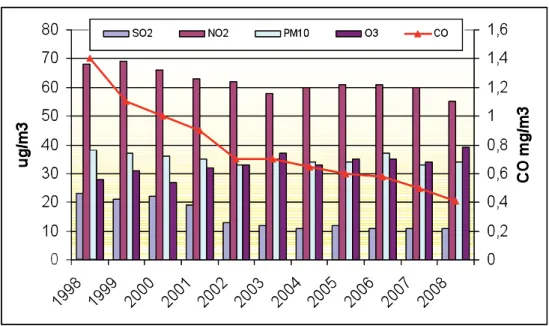
of the atmosphere. Tropospheric ozone (often termed “bad” ozone) is man-made, a result of air pollution from internal combustion engines and power plants. Automo-bile exhaust and industrial emissions release a family of nitrogen oxide gases (NOx) and volatile organic compounds (VOC), by-products of burning gasoline and coal. High levels of ozone are usually formed in Madrid in the heat of the afternoon and early evening, dissipating during the cooler nights. Figure 2 shows the annual ten-dency of these pollutants in the last ten years.
Figure 2. Sulphur dioxide, Nitrogen dioxide, Carbon monoxide, Particulate matter (PM10) and Ozone. Madrid (1998-2008)
Source: Report on Air Quality in Madrid. 2008. General Direction for Environmental Quality,
Control and Assessment. Municipality of Madrid.
3.2. Data set
The objective data used in this paper have been provided for the Atmosphere Pollution Monitoring System of Madrid municipality2. They have been hourly
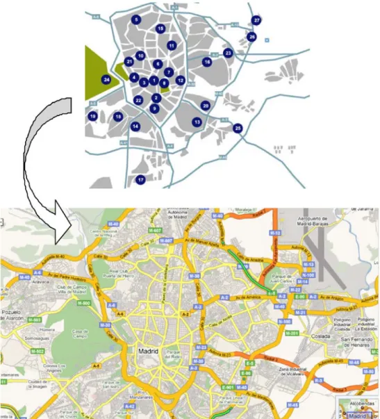
measured at the 25 fixed operative monitoring stations during January, 2008 (a month with dense traffic and low temperatures). Figure 3 shows the locations of
2 Information of these data can be obtained from the Municipality of Madrid’s web page at www.munimadrid.es
the air quality monitoring stations, and Table 1 includes address, municipal dis-trict, and coordinates and altitude level of such stations.
As can be seen in Figure 3, most monitoring stations are located in the urban centre and relatively few in the peripheral sites. Note the reasonable coverage of the domain under study by the monitoring stations since most of Madrid popula-tion is concentred in the urban centre.
Table 1. A tmosphere pollution monitoring stations in Madrid Station A ddress District Longitude latitude altitude (meters) Characteristics 01 Paseo Recoletos Centro 3º41’31.00’’ 40º25’21.36’’ 678 City centre, financial area, high traffic site 03 Pl. del Car men Centro 3º42’11.42’’ 40º25’09.15’’ 657 City centre, commercial area, pedestrian zone with ver y limited traffic 04 Pl. de España Moncloa 3º42’44.40’’ 40º25’26.37’’ 637 City centre, commercial area, high traffic site 05 Bar rio del Pilar Fuencar ral 3º42’41.56’’ 40º28’41.62’’ 673 North part of the city , commercial area, high traffic site 06 Pl. Dr . Marañon Chamberí 3º41’27.00’’ 40º26’15.39’’ 669 City centre, commercial area, high traffic site 07 Pl. M. Salamanca Salamanca 3º40’49.19’’ 40º25’47.81’’ 679 Residential and commercial area, high traffic site high income level 08 Escuelas Aguir re Salamanca 3º40’56.35’’ 40º25’17.63’’ 672 high traffic site, but opposite to the biggest green area in the city 09 Pl. Luca de Tena Arganzuela 3º41’36.35’’ 40º24’07.68’’ 605 South part of the central almond, near to the inner ring road of the city 10 Cuatro Caminos Chamberí 3º42’25.66’’ 40º26’43.95’’ 699 City centre, commercial area, high traffic site, old buildings 11 A v. Ramón y Cajal Chamartín 3º40’38.47’’ 40º27’05.30’’ 708 North part of the city , near to a highway , dispersed build-up. 12 Plaza Manuel Becer ra Salamanca 3º40’06.78’’ 40º25’43.70’’ 678 South part of the city , high traffic site, near to the inner ring road of the city 13 Vallecas Puente Vallecas 3º39’05.48’’ 40º23’17.34’’ 677 South part of the city , high traffic site, intensive build-up, low income level 14 Plaza Fdez. Ladrada Usera 3º42’59.71’’ 40º23’06.28’’ 605 South part of the city , intensive build-up, high traffic site, industries, ver y low income level.
Station A ddress District Longitude latitude altitude (meters) Characteristics 15 Pl. de Castillla Tetuán/ Chamartín 3º41’19.29’’ 40º28’05.73’’ 729 North part of the city , institutions, high income level, dispersed build-up, high traffic site 16 Arturo Soria Ciudad Lineal 3º38’21.24’’ 40º26’24.17’’ 698 North-East part of the city , high income level, dispersed build-up 18 General Ricardos Carabanchel 3º43’54.60’’ 40º23’41.20’’ 625 South-W est part of Madrid, populous area, intensive build-up, low income level 19 Alto Extremadura Latina 3º44’30.83’’ 40º24’28’.29’’ 632 W est part of Madrid, green areas, dispersed build-up 20 A v. Moratalaz Moratalaz 3º38’43.06’’ 40º24’26.64’’ 671 East part of the city , intensive build-up, medium income level 21 Isaac Peral Moncloa 3º43’04.54’’ 40º26’24.51’’ 672 W est part of Madrid, near to an important highway 22 Paseo de Pontones Arganzuela 3º42’46.56’’ 40º24’22.95’’ 622 Ne xt to the city centre, near to the inner ring road of the city 23 Alcalá (end) San Blas 3º36’34.62’’ 40º26’55.44’’ 637 North-East part of Madrid, populous area, intensive build-up, low income level 24 Casa de Campo Moncloa 3º44’50.44’’ 40º25’09.68’’ 645 Main green area in the city 25 Santa Eugenia V illa Vallecas 3º36’09.18’’ 40º22’44.48’’ 652 South-East part of the city , old buildings, industries, near one important highway , ver y low income level 26 Urb. Embajada Barajas 3º34’48.42’’ 40º27’33.56’’ 620 North-East part of the city , near the airport, dispersed build-up 27 Barajas Pueblo Barajas 3º34’48.10’’ 40º28’36.94’’ 631 North-East part of the city , near the airport, intensive build-up Source: General Direction for Environmental Quality , Control and Assessment. Municipality of Madrid. (*) Pl.: Square. A v: A venue. Urb: con -dominium. Monitoring Stations 17 and 2 are not operative.
For each hour, data have been daily averaged. As can be seen in Table 2, the range, mean, and standard deviation of the six daily averaged (objective) variables considered in the analysis considerably vary. This is the reason why data have been standardised. Summing up, we work with 24 hourly data sets, each one in-cluding six environmental variables.
Table 2. Environmental variables: Main descriptive statistics
Min. Max. Mean deviationStandard SO2(a) 10.11 21.84 15.99 5.17 NOx(a) 66.82 238.65 150.10 40.85 NO2(a) 37.14 99.79 69.01 14.16 PM(a) 13.44 49.08 32.16 8.75 O3(a) 9.75 24,65 15.50 3.49 CO(b) 0.31 0.86 0.58 0.18 (a): μ/m3; (b): mg/m3 Source: Own elaboration.
In the literature of making EQIs, it is usual to average the hourly data and obtain monthly averages of the level of pollutants. Evidently, it makes easier the task of elaborating EQIs, but we have preferred not to use monthly averaged data because: (i) the spatial structure of dependencies is not the same every hour, and the averaging process could lead to compensate such different structures. (ii) Pro-ceeding in this way, we have at our disposal 24 data sets to empirically compare the usual way of predicting EQIs with the alternative we propose.
Subjective information for areas (census tracks) has been derived from the results of a questionnaire referring to pollution perceptions, the respondents be-ing aware that, supposedly, they were to buy a house. The number of responses was 5,300.
Variables included in the drift were the number of urban road kilometres, proximity to the main radial highways, M-30 first belt, and M-40 second belt, number of coal boilers that still work with coal in a radius of 250 meters, number of houses, number of offices, number of commercial premises, altitude, and prox-imity to a green area (weighted by the size of that area). The basic information was obtained from the Population and Houses Spanish Census; the number of coal boilers and their location was facilitated by the Council of Madrid; and dis-tances are own calculations.
Finally, note that in the specialized literature hedonic specifications typi-cally include only one air pollutant such as ground-level ozone (O3) –Banzhaf, 2005, Hendrix, 2005, Anselin, 2006–, or particulate matter (PM) –Chay,
Green-stone, 2005, Murthy et al., 2007–, since these are most visible in the form of “smog” and are thought to have the greatest health impacts. In some cases, the variables included are two (Neill et al., 2007, which include carbon monoxide (CO) and PM, and Anselin and Lozano-Gracia, 2008, which consider the meas-ures of O3 and PM concentrations, are recent examples) or, at most, three, in order to minimize omitted variable problems. But a viable treatment of environ-mental data should consider multiple contaminants. Obviously, the incorpora-tion of six (or more) variables to a hedonic house price model is not an easy task, and it is preferred to incorporate an environmental index that gathers the information contained in such variables.
3.3. Kriging modelling, results, and discussion
As it was pointed out in the introduction, it is more and more frequent the use of environmental variables as explanatory variables in hedonic housing price models. But if the number of environmental variables is more than one, it is a common practice to elaborate EQIs that condense the information provided for the environmental variables, so that only one environmental variable (EQI) is in-cluded in the model. However, the number of housing prices is much larger than the number of monitoring stations.
Additionally, people’s perceptions about pollution are core information, be-cause it is really the component that enters in the utility function of the potential owners of the property. The combination of both objective (in a punctual support) and subjective information (in a block support) leads to a coherence problem, which modifies the usual expression of the kriging predictor.
In particular, in our study case (Madrid City) we deal with six environmen-tal variables (so, an EQI is needed), and the number of monitoring stations is 25, while, for example, official statistics provide mean housing prices in the 2,358 cen-sus tracks of Madrid. This mismatching leads to the prediction of EQI values at the locations (punctual or block locations as census tracks) where there is not en-vironmental information at our disposal. As also pointed out in the introductory section, several interpolative alternatives have been considered in recent research, but when dealing with environmental variables kriging has important advantages, because it takes into account the spatial dependencies, what is crucial to obtain optimal predictions when dealing with geo-referred data (Bokwa, 2008, Hooy-berghs et al., 2006, are good examples of the advantage of kriging over the other interpolative methods in the environmental field).
The classical geostatistical model assumes that data are Gaussian. In the Gaus-sian case, as it is well known, the optimal predictor (taking the mean square error as a loss function) is linear and coincides with kriging predictor. This assumption may be certainly strong for some data sets, but in our particular standardized data set Gaussian transformation has been no needed. Also, UTM coordinates have been transformed in [0–1]×[0–1] coordinates to easily interpret the resulting em-pirical semivariograms.
Once decided that kriging is the appropriate strategy to match the monitoring stations registers to the housing prices data, and standardized the environmen-tal variables, we next face and compare the usual approach in the literature (first elaborate an EQI and then obtain kriged predictions of the EQI) to the alterna-tive approach we propose. With regard to this alternaalterna-tive approach, in a first step we krige the objective environmental variables to obtain predictions in the desired locations and finally, we elaborate the environmental index. In a second step, we include the subjective information and compute the A2PKED MEQI following the same path as previously. In order to build the final synthetic index, we use Princi-pal Components Analysis (PCA), as usual in the literature.
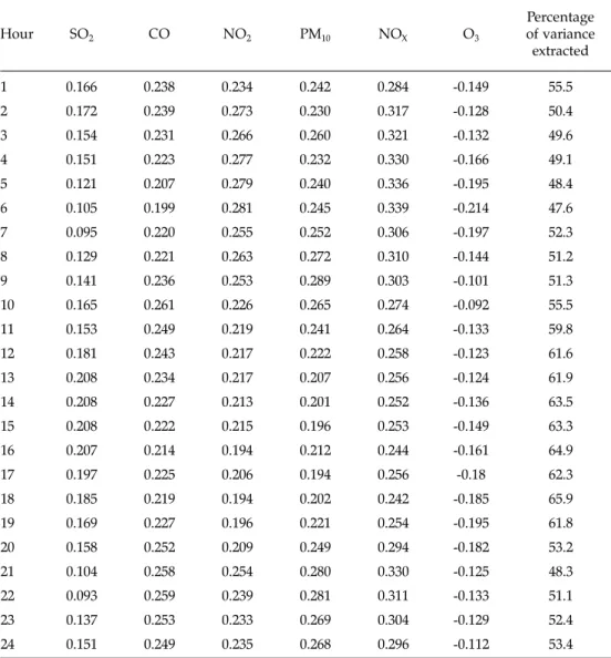
When it comes to implement the traditional approach, in a first stage we pro-ceed to elaborate what we call the “standardized observed EQI”. That is, we apply PCA to the six standardized environmental variables at our disposal and extract the first component, obtaining the coefficients for the environmental variables in the observed EQI3 (see Table 3). Finally, the values of the observed EQI are com-puted for every monitoring station and every hour.
In a second stage, krided predictions of the observed index have been ob-tained in the locations equipped with a monitoring station. A cross-validation procedure has been carried out to obtain such predictions. Spatial dependencies have been represented by Gaussian variograms from 01a.m to 06a.m, exponential variograms (with one exception) between 07a.m. and 04p.m., and spherical mod-els from 05p.m to 12p.m. Except from 11a.m. to 18p.m., there are notable nugget effects, and ranges are, in average, around 20 percent of the domain longitude.
In the third and last stage, these predictions (one for each hour and each monitoring station) are compared to the observed EQI values, and hourly MSE are computed. Table 4 reports these hourly MSE.
Alternatively, we proceed to implement a new approach consisting of:
1. Obtaining, by a cross-validation procedure, kriging predictions of the envi-ronmental variable values at locations where monitoring stations are sited in Madrid City. We first have computed the 144 classical empirical variograms, which have being represented by their corresponding theoretical models. In particular, most of semivariograms representing the spatial dependencies of levels of SO2 and CO levels were exponential. In the case of NO2 and PM10
most of variograms were spherical. When dealing with the spatial dependen-cies in the NOx case the semivariograms used to be Gaussian. And finally, the
O3 spatial dependence was modelled by Spherical semivariograms in the night
hours and Exponential ones from 9 a.m. to 8 p.m.
2. Weighting the predictions of the environmental variable values with the co-efficients obtained through PCA, and computing the predicted EQI for each hour and each monitoring station.
3. Comparing the EQI predicted and observed values and computing hourly MSE. 3 The averaged percentage of the total variance extracted with the first component is 55.6%.
Finally, we have implemented the previous alternative combining punctual objective environmental variables with areal subjective air pollution information and solving the coherence problems by using a A2PKED predictor (as shown in the methodological Section). Selected variograms does not differ significantly from the ones obtained in the previous approach.
Table 4 shows the hourly MSE derived from the usual and the two alternative approaches to estimating an EQI (or MEQI in case of including both objective and subjective information) for Madrid City.
Table 3. Environmental variable coefficients in EQI (ACP)
Hour SO2 CO NO2 PM10 NOX O3 Percentage of variance extracted 1 0.166 0.238 0.234 0.242 0.284 -0.149 55.5 2 0.172 0.239 0.273 0.230 0.317 -0.128 50.4 3 0.154 0.231 0.266 0.260 0.321 -0.132 49.6 4 0.151 0.223 0.277 0.232 0.330 -0.166 49.1 5 0.121 0.207 0.279 0.240 0.336 -0.195 48.4 6 0.105 0.199 0.281 0.245 0.339 -0.214 47.6 7 0.095 0.220 0.255 0.252 0.306 -0.197 52.3 8 0.129 0.221 0.263 0.272 0.310 -0.144 51.2 9 0.141 0.236 0.253 0.289 0.303 -0.101 51.3 10 0.165 0.261 0.226 0.265 0.274 -0.092 55.5 11 0.153 0.249 0.219 0.241 0.264 -0.133 59.8 12 0.181 0.243 0.217 0.222 0.258 -0.123 61.6 13 0.208 0.234 0.217 0.207 0.256 -0.124 61.9 14 0.208 0.227 0.213 0.201 0.252 -0.136 63.5 15 0.208 0.222 0.215 0.196 0.253 -0.149 63.3 16 0.207 0.214 0.194 0.212 0.244 -0.161 64.9 17 0.197 0.225 0.206 0.194 0.256 -0.18 62.3 18 0.185 0.219 0.194 0.202 0.242 -0.185 65.9 19 0.169 0.227 0.196 0.221 0.254 -0.195 61.8 20 0.158 0.252 0.209 0.249 0.294 -0.182 53.2 21 0.104 0.258 0.254 0.280 0.330 -0.125 48.3 22 0.093 0.259 0.239 0.281 0.311 -0.133 51.1 23 0.137 0.253 0.233 0.269 0.304 -0.129 52.4 24 0.151 0.249 0.235 0.268 0.296 -0.112 53.4
Table 4. Traditional and alternative approaches for estimating EQIs. MSE estimating an EQI for Madrid City (Spain)
Hour Kiriging the EQI MSE (i) Kriging Enviromental Variables MSE (ii) A2P-kriging the MEQI MSE(iii)
MSE (i)-MSE (ii) MSE (ii)-MSE (iii)
1 0.99 0.82 0.72 0.17 0.10 2 0.87 0.82 0.63 0.05 0.19 3 1.02 0.86 0.71 0.16 0.15 4 0.75 0.77 0.74 -0.02 0.03 5 0.83 0.83 0.83 0.00 0.00 6 0.96 0.96 0.83 0.00 0.13 7 1.08 1.07 1.01 0.01 0.06 8 1.09 1.07 0.95 0.02 0.12 9 1.05 1.00 0.83 0.05 0.17 10 0.96 0.91 0.76 0.05 0.15 11 0.87 0.85 0.71 0.02 0.14 12 0.72 0.72 0.69 0.00 0.03 13 0.57 0.57 0.55 0.00 0.02 14 0.53 0.54 0.49 -0.01 0.05 15 0.56 0.58 0.50 -0.02 0.08 16 0.54 0.55 0.51 -0.02 0.04 17 0.66 0.67 0.56 -0.01 0.11 18 0.75 0.72 0.61 0.03 0.11 19 1.06 0.89 0.79 0.17 0.10 20 1.09 0.98 0.76 0.11 0.22 21 1.08 1.07 0.77 0.01 0.30 22 1.08 1.05 0.90 0.03 0.15 23 1.05 0.93 0.76 0.12 0.17 24 1.00 0.87 0.68 0.13 0.19 Total 0.89 0.84 0.72 0.05 0.12
Source: Own elaboration.
As expected, in Table 4 it can be appreciated that the alternative consisting of kriging the objective variables and subsequently elaborating the EQI gives bet-ter results in 15 out of 24 hours: from 06p.m. to 03a.m. (both included) and from 07a.m. to 11a.m. (also both included). From 05a.m. to 06a.m. and from 12a.m. to
01p.m. results were practically identical. And at 04a.m. and from 02p.m. to 05p.m. the traditional procedure has a negligible advantage (just the hours when spatial dependencies are softer). Then, the alternative approach generates less MSE than the classical procedure in the hours when traffic is dense and/or heating is work-ing. In particular, the reduction of MSE in the hours most affected by traffic and/ or heating (between 07p.m. and 03a.m.) using the new procedure is by 10.6%. From 07a.m. to 11a.m. (hours with a high level of economic activity in Madrid City) the reduction in MSE is by 3%, but it has to be considered that in this hourly lag the spatial dependencies are not precisely strong.
If areal subjective information is taken into account, it can be appreciated an additional reduction in the prediction MSE by 12%. By using A2PKED strategy with both objective and subjective air pollution information the prediction MSE diminish in all the hours of the day, the additional diminishing being of above 15% in the hours when traffic is dense and/or heating is working. Newly, the big-ger are the spatial dependencies, the larbig-ger is the reduction in MSE.
Therefore, it can be appreciated that, in general, the alternative consisting of kriging the objective variables and subsequently elaborating the EQI has better results, in terms of MSE, than the traditional one (elaborating the EQI and then kriging this EQI). Additionally, if subjective air pollution variables are included in the analysis and both objective and subjective information are linked through a A2PKED strategy, the prediction MSE declines substantially, and the stronger the spatial dependencies are, the bigger the advantage of the A2PKED strategy com-bined with the alternative consisting of kriging the objective variables and sub-sequently elaborating the EQI is. In general, our proposal reduces the prediction MSE by a 17% relative to the traditional procedure in the literature. In the most “problematic” hours, this reduction reaches the 30%.
4. Concluding remarks and future research
Hedonic housing price models with explanatory environmental variables are becoming more and more popular due to a substantial body of research that em-pirically confirms the hedonic theory and suggests that consumers are willing to pay for environmental goods. Typically, only one or at most two or three en-vironmental variables are considered in hedonic housing price models. However, a viable treatment of environmental data should consider multiple contaminants. We have incorporated six pollutants and, as far as we know, there are no research considering six environmental variables, as here is done. Obviously, the incorpora-tion of six (or more) variables in a hedonic house price model is not an easy task, and it is preferred to incorporate an environmental index that gathers the infor-mation contained in such variables.
But the main problem to incorporate environmental variables in a house pric-es hedonic model is that the number of locations where a property transaction has been taken place is very much denser than the number of locations equipped with an environmental monitoring station. Kriging the environmental information
in the locations where house prices are at our disposal but not equipped with a monitoring station is the usual solution to this problem.
To be more precise, in the literature the usual way to solve the above-mentioned problem is the elaboration of an environmental quality index (EQI), and then in-terpolating it (preferably kriging) in the locations where house prices are available and pollutants have not been measured. But in this article it is proposed the inverse procedure, i.e. to interpolate the environmental variables and, subsequently, elabo-rate an EQI, because the prediction variance is lesser. An additional problem is that environmental information can be both objective (measures provided by monitor-ing stations) or subjective (people’s perceptions). In this sense, mixed EQIs (ME-QIs) are preferred. In the literature, hedonic strategies usually only include objec-tive environmental variables but subjecobjec-tive variables are also crucial when it comes to estimate the impact of pollution on housing prices. The problem now arises is the mismatch between the spatial support for the environmental objective informa-tion (punctual support, the locainforma-tions equipped with a monitoring stainforma-tion) and the subjective information (block support, usually census tracks). But this problem can be transformed in an advantage if it is designed a kriging strategy that links objec-tive environmental information (scarce) with subjecobjec-tive one (dense in the sense that it represent the mean of a particular area). This is the reason why in this article a version of universal kriging that combines the information coming from different sources has been proposed (area- to-point kriging with external drift).
In this research we have empirically compared both the traditional and the al-ternative approaches by elaborating an EQI for Madrid City (Spain). The database includes 24 daily averaged (January 2008) datasets, one per hour. As a first result, in the hours when traffic is denser and/or heating is working the alternative con-sisting of kriging the objective air pollution variables and subsequently computing the EQI has a notable advantage, while in the rest of the hours both procedures generate similar results. A second and more important result is that the combina-tion of areal subjective informacombina-tion with punctual objective data, both co-existing in a coherent way by using a A2PKED strategy, leads to an additional substantial reduction in the prediction MSE (17% relative to the traditional procedure in the literature, and more than 30% in the hours when pollution is higher). But, per-haps, the most important insight is that the stronger the spatial dependencies are, the bigger the advantage of the alternative procedure is.
This case study empirically confirms an important aspect of the geostatisti-cal theory when dealing with several variables and the objective is to transform a multivariate problem in a univariate one: In general, prediction MSE is lesser when interpolating the variables involved in a linear combination and then elabo-rating such a linear combination. But the literature continues to obviate this im-portant result and the usual procedure is to first elaborating the linear combina-tion and then interpolating it. The analyzed case study also statistically confirms the intuition that people’s perception about pollution is crucial when it comes to predict the level of pollution (represented by an EQI) across a particular spatial domain. Obviously, our research includes only a case study and our results must be confirmed in other big cities and in different months.
Finally, there are at least four important aspects that could give rise to future research lines: (i) the elaboration of a statistical location design of the network of monitoring stations to reduce the most as possible the variance of the prediction error; (ii) the inclusion of source-receptor matrices in the analysis to take into ac-count the way in which atmospheric influences distort the source-receptor distri-bution (i.e. how pollution “travels” from the source of emission (point sources or mobile sources) to where it is measured; (iii) the elaboration of spatial-temporal EQI’s that takes into account not only the spatial dependencies but also the tem-poral ones and the interaction of space and time; and (iv) the elaboration of func-tional EQI’s, which would predict smooth time functions of pollution at each loca-tion, instead of punctual predictions.
Aknowledgements
Comments and suggestions from Hans Wackernagel, Xavier Emery, Jorge Ma-teu and Emilio Porcu on the standard deviation of the prediction error provided by kriging and cokriging are gratefully acknowledged. The authors are responsi-ble for any remaining errors. This research has been partially founded for Junta de Comunidades de Castilla-La Mancha, under FEDER research project PAI-05-021.
References
Anselin L. and Le Gallo J. 2006. Interpolation of Air Quality Measures in Hedonic House Price Models: Spatial Aspects. Spatial Economic Analysis 1-1: 31-52.
Anselin L. and Lozano-Gracia N. 2008. Errors in variables and spatial effects in hedonic house price models of ambient air quality. Empirical Economics 34: 5-34.
Banzhaf H.S. 2005. Green Price Indices. Journal of Environmental Economics and Management 49 (2): 262-280.
Bayer C., Lovato T., Dieckow J., Zanatta J.A. and Mielniczuk, J. 1996. A.method for estimating coefficients of soil organic matter dynamics based on long-term experiments. Soil and Tillage Research 91: 217-226.
Braden J.B. and Kolstad C.K. 1991. Measuring the demand for environmental quality. Amsterdam, North-Holland.
Bokwa A. 2008. Environmental Impacts of Long-Term Air Pollution Changes in Kraków, Poland. Polish Journal of Environmental Studies 17 (5): 673-686.
Chay K.Y. and Greenstone M. 2005. Does air quality matter? Evidence from the housing market.
Journal of Political Economy 113(2): 376-424.
Chilès J.P. and Delfiner P. (1999). Geostatistics. Modeling Spatial Uncertainty. Wiley, New York. De Iaco S., Myers D.E. and Posa D. 2001. Total air pollution and space–time modeling. In:
Mone-stiez, P., Allard, D., Froidevaux, R. (Eds.), GeoEnv III – Geostatistics for Environmental Applica-tions, Kluwer Academic Publishers: Dordrecht, pp 45–56.
De Iaco S., Myers D.E. and Posa D. 2002. Space-time variograms and a functional form for total air pollution measurements. Computational statistics & Data Analysis 41: 311-328.
Emery X. 2000. Geoestadística lineal. Departamento de Ingeniería de Minas. Facultad de CC. Físi-cas y MatemátiFísi-cas, Universidad de Chile [In Spanish].
Freeman III A. M. 1993. The measurement of environmental and resource values: theory and methods, Resources for the future. Washington, D. C.
Hendrix M.E., Hartley P.R. and Osherson D. 2005. Real Estate Values and Air Pollution: Measured Levels and Subjective Expectations; Discussion Paper, Rice University.
Hooyberghs J., Mensink C., Dumontb G. and Fierensb F. 2006 Spatial interpolation of ambient ozone concentrations from sparse monitoring points in Belgium. Journal of Environmental Mo-nitoring 8: 1129–1135.
Kim C-W., Phipps T.T. and Anselin L. 2003. Measuring the benefits o fair quality improvement: A spatial hedonic approach. Journal of Environmental Economics and Management 45: 24-39. Lark R.M. and Papritz A. 2003. Fitting a linear model of corregionalization for soil properties
using simulate annealing. Geoderma 115: 245-260.
Montero J.M. and Larraz B. 2006. Estimación espacial del precio de la vivienda mediante méto-dos de krigeado. Revista Estadística Española 48 (162): 62-108 [In Spanish].
Montero J.M. and Larraz B. 2008. Introducción a la geoestadística lineal, A Coruña: Netbiblo [In Spa-nish].
Murthy M.N., Gulati S.C. and Banerjee. A. 2007. Hedonic property prices and valuation of benefits from reducing urban air pollution in India. Discussion Papers 61, Institute of Economic Growth, India, Delhi.
Myers D.E. 1983. Estimation of linear combinations and cokriging. Mathematical Geology 15: 633-637. Neill H.R., Hassenzahl D.M. and Assane D.D. 2007. Estimating the effect of air quality: spatial
versus traditional hedonic price models. Southern Economic Journal 73 (4): 1088-1111.
Preisendorfer R.W. 1998. Principal Component Analysis in meteorology and oceanography. Amsterdam, Elsevier.
Spence J. S., Carmack P. S., Gunst R. F., Schucany W. R.Woodward, W.A. and Haley W. 2007. Ac-counting for Spatial Dependence in the Analysis of SPECT Brain Imaging Data. Journal of the American Statistical Association 102: 464–473.
Smith V.K. and Huang J.C. 1993. Hedonic models and air pollution: twenty-five years and counting. Environmental and Resource Economics 36-1: 23-36.
Smith V.K. and Huang J.C. 1995. Can markets value air quality? A meta-analysis of hedonic pro-perty value models. Journal of Political Economy 103: 209-227.
Smith V.K. and Kaoru Y. 1995. Signals or noise-explaining the variation in recreation benefit esti-mates. American Journal of Agricultural Economics 72: 419-433.
Statheropoulos M., Vassiliadis, N. and Pappa A. 1998. Principal component and Canonical corre-lation analysis for examining air pollution and meteorological data. Atmospheric Environment
6: 1087–1095.
Subramanyam A. and Pandalai H.S. 2004. On the equivalence of the cokriging and kriging sy-stems. Mathematical Geology 36 (4): 507-523.
Tzeng S., Huang H.C. and Cressie, N. 2005. A fast, optimal spatial-prediction method for massive datasets. Journal of the American Statistical Association 100: 1343-1357.
Wakernagel H. 1998 Principal component analysis for autocorrelated data: a geostatistical perspective. Technical report, Centre de Geostatistique, Ecole de Mines de Paris: Fontainebleau.
Wong D.W., Yuan L. and Perlin S.A. 2004. Comparison of spatial interpolation methods for the estimation of air quality data. Journal of Exposure Analysis and Environmental Epidemiology 14: 404–415.