Sensitivity Analysis For The Winning Algorithm In Knowledge Discovery And Data Mining (kdd) Cup Competition 2014

(1)

Illinois State University

ISU ReD: Research and eData

Theses and Dissertations

3-16-2015

Sensitivity Analysis For The Winning Algorithm In

Knowledge Discovery And Data Mining (kdd)

Cup Competition 2014

Fakhri Ghassan Abbas

Illinois State University, fakhri.g.abbas@gmail.com

Follow this and additional works at:http://ir.library.illinoisstate.edu/etd

Part of theDatabases and Information Systems Commons

This Thesis and Dissertation is brought to you for free and open access by ISU ReD: Research and eData. It has been accepted for inclusion in Theses and Dissertations by an authorized administrator of ISU ReD: Research and eData. For more information, please contactISUReD@ilstu.edu.

Recommended Citation

Abbas, Fakhri Ghassan, "Sensitivity Analysis For The Winning Algorithm In Knowledge Discovery And Data Mining (kdd) Cup Competition 2014" (2015).Theses and Dissertations.Paper 347.

(2)

SENSITIVITY ANALYSIS FOR THE WINNING ALGORITHM IN KNOWLEDGE DISCOVERY AND DATA MINING (KDD) CUP COMPETITION 2014

Fakhri G. Abbas

60 Pages May 2015

This thesis applies multi-way sensitivity analysis for the winning algorithm in the Knowledge Discovery in Data Mining (KDD) cup competition 2014 -‘Predicting

Excitement at Donors.org’. Because of the highly advanced nature of this competition, analyzing the winning solution under a variety of different conditions provides insight about each of the models the winning team has used in the competition. The study

follows Cross Industry Standard Process (CRISP) for data mining to study the steps taken to prepare, model and evaluate the model. The thesis focuses on a gradient boosting model. After careful examination of the models created by the researchers who won the cup, this thesis performed multi-way sensitivity analysis on the model named above. The sensitivity analysis performed in this study focuses on key parameters in each of those algorithms and examines the influence of those parameters on the accuracy of the predictions.

(3)

FAKHRI G. ABBAS

A Thesis Submitted in Partial Fulfillment of the Requirements

for the Degree of MASTER OF SCIENCE Department of Information Technology

ILLINOIS STATE UNIVERSITY 2015

(4)

(5)

FAKHRI G. ABBAS

COMMITTEE MEMBERS: Elahe Javadi, Chair

(6)

i

ACKNOWLEDGMENTS

I would like to express my deepest appreciation for the committee chair Dr. Elahe Javadi and Dr. Bryan Hosack who guided me through the process of completing this work. Without their guidance and help this thesis would not have been possible. Also I would like to thank the technical team in the Information Technology department who helped me by providing resources to run and simulate the model.

(7)

ii CONTENTS Page ACKNOWLEDGMENTS i CONTENTS ii TABLES iv FIGURES v CHAPTER

I. THE PROBLEM AND ITS BACKGROUND 1

Statement of the Problem 1

Hypotheses 1

Definition of Terms 2

Limitations of the Study 2

Methodology 3

Collection of the Data 3

Analysis of the Data 3

II. REVIEW OF RELATED LITERATURE 5

General Literature Review 5

Introduction to Data Mining 5

Cross Industry Standard Process for Data Mining 7

Sensitivity Analysis 9

Specific Research 11

Data Mining Classification and Regression Models 11

The Problem of Overfitting 12

Gradient Boosting 13

General Themes 16

(8)

iii

III. RESEARCH DESIGN 19

Research Design Procedures 19

Applying CRISP-DM Approach 21

Collection of the Data 28

Materials 28

Measurements 28

Assessments 28

IV. ANALYSIS OF THE DATA 29

Statistical Analysis 29

Findings and Results 30

Selecting Shrinkage Value 30

Number of Trees and Interaction Depth Values 31

Summary 39

V. SUMMARY, CONCLUSIONS, AND

RECOMMENDATIONS 41

Summary of the Research Problem,

Methods and Findings 41

Conclusions and Implications 41

Recommendations for Future Research 44

REFERENCES 45 80

APPENDIX A: DATA DESCRIPTION 48

APPENDIX B: GBM R PACKAGE 54

APPENDIX C: SENSITIVITY ANALYSIS SOURCE CODE 58

APPENDIX D: AUTOMATE UPLOADING PROCESS 59

APPENDIX E: SHRINKAGE VALUE SOURCE CODE 60

(9)

iv TABLES

Table Page

1. Shrinkage, Number of Trees and Interaction

Depth - Baseline Values Parameters 25

2. Summary of Parameters Values the Study Focuses On 27

3. Comparing Old and New Results 35

4. Results with Shrinkage 0.1 40

(10)

v FIGURES

Figure Page

1. UML Diagram for Dataset 4

2. The Cross Industry Standard Process is an Iterative and Adaptive 8

3. Shrinkage Value with 500 Trees and Depth of 5 31

4. GBM 1 Results: Maximum Accuracy at 600 Trees with Depth 5 32 5. GBM 2 Results: Maximum Accuracy at 300 Trees with Depth 11 33 6. GBM 3 Results: Maximum Accuracy at 950 Trees with Depth 3 34 7. GBM 4 Results: Maximum Accuracy at 1000 Trees with Depth 3 35

8. GBM 1 Results 36

9. GBM 2 Results 37

10. GBM 3 Results 38

(11)

1 CHAPTER I

THE PROBLEM AND ITS BACKGROUND Statement of the Problem

Knowledge Discovery and Data Mining (KDD) hosts an annual competition in which a data science problem is presented. The competition challenges the participants to provide the best solution in the context of data mining and knowledge discovery. In KDD Cup 2014, participants asked to build a model that predicts the most exciting projects located under DonorsChoose.org for donors to donate and implement. The winning algorithm’s accuracy was 0.67814, which is very close to the second and third, 0.67320 & 0.67297 respectively. However, the winning algorithm and documentation lack a justification for the parameters used to evaluate the model that produced the results. This study follows Cross Industry Standard Process (CRISP) to address the stated problem and uses sensitivity analysis to come up with a model with tuned parameters which increases the accuracy.

Hypotheses

This study focused on three parameters for GBM. In addition to that, multi-way sensitivity analysis used to tune the parameters.

 H1: Increasing the number of trees in GBM model will increase model’s accuracy until the model starts to overfit the data.

(12)

2

 H2: Increasing the interaction depth in GBM model will increase model’s accuracy until the model starts to overfit the data.

 H3: The relation between number of trees and interaction depth is inverse relation and could be tuned to increase the GBM model’s accuracy.

 H4: Shrinkage value optimized in GBM model based on memory available Definition of Terms

KDD: Knowledge Discovery and Data Mining

CRISP: Cross Industry Standard Process for Data Mining OLAP: Online Analytic Processing

ICDM: IEEE International Conference on Data Mining CART: Classification and Regression Trees

GBM: Gradient Boost Machine GPL: General Public License

AAAI: Association for the Advancement of Artificial Intelligence CSV: Comma Separated Values

TF-IDF: Text Frequency – Inverse Document Frequency Limitation of the Study

The lack of documentation of the winning algorithm was a major challenge to understand the implemented model. In addition to that, the excessive amount of memory usage for the model makes it very hard to run over the existing instance of R studio. Therefore, minor modifications were introduced to the existing model by releasing the memory whenever there is no need to hold it anymore.

(13)

3

The lack of resources for the current R Studio server prevent evaluation of Extremely Randomized Tree model and make the study limited to the Generalized Boosted Regression Model.

Methodology

The CRISP data mining process followed to address the problem statement stated above with focus on model evaluation phase. The evaluation process conducted using multi-way parameter sensitivity analysis. In which, multiple parameters values studied to determine the best combination of the parameters that has best effect on the model. The models divided to multiple models in which each model studied independently. For each model, different combinations of parameters applied to study and compare the results associated with each combination.

Collection of Data

Kaggle provides a dataset for projects along with their donations, essays, resources and outcomes for projects up to 2013 as a training set, while the testing set includes projects after 2013 till mid May 2014 excluding already live projects. The data supplied by DonorsChoose.org - an online charity that makes it available for anyone to help student through online donations. The data used for the competition is available for public to download and analyze through the KDD Cup 2014 competition website.

Analysis of the Data

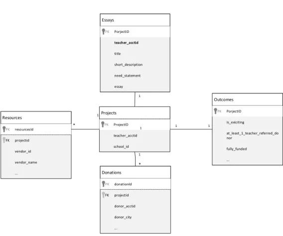
The data comes into comma separated values files (csv). Each file corresponds to one entity which includes:

(14)

4

 Resources each row represents a resource used by the project. Same project might have multiple resources.

 Donations (training set only) each row represent a donation related to single project. Same project might have multiple donations.

 Essays each row represents the essay part related to single project.

 Outcomes (training set only) the result for the training set it has projectid along with whether the project is exciting or not.

The following diagram identifies the relation between all entities.

Projects ProjectID PK Essays PorjectID PK Resources resourcesId PK projectid FK Donations donationId PK projectid FK 1 1 1 1 * * Outcomes PorjectID PK 1 1 teacher_acctid title need_statement short_description essay vendor_id vendor_name ... donor_acctid donor_city ... at_least_1_teacher_referred_do nor fully_funded ... is_exiciting teacher_acctid school_id

(15)

5 CHAPTER II

REVIEW OF RELATED LITERATURE General Literature Review

Introduction to Data Mining

Data mining defined as “the process of discovering meaningful new correlations, patterns and trends by sifting through large amounts of data stored in repositories, using pattern recognition technologies as well as statistical and mathematical techniques.” (Thearling, 1999). It includes an in-depth analysis of data include building a prediction models. The analysis identified goes beyond the aggregation functions in relational database and Online Analytic Processing (OLAP) servers. It includes algorithms such as, decision trees, linear and logistic regression, neural networks and more (Chaudhuri, Dayal, & Narasayya, 2011).

In one effort of identifying the top data mining algorithms, the IEEE International Conference on Data Mining (ICDM) identified the top 10 algorithms in data mining for presentation at ICDM 2006 at Hong Kong. The algorithms organized in 10 categories: association analysis, classification, clustering, statistical learning, bagging and boosting, sequential patterns, integrated mining, rough sets, link mining, and graph mining. The top 10 algorithms are: C4.5, k-mean algorithm, Support Vector Machine, The Apriori

algorithm, The EM algorithm, PageRank, AdaBoost, k-nearest neighbor classification, Naïve Bayes, CART “Classification and Regression Trees” (Wu et al., 2008).

(16)

6

The main tasks that data mining is usually called upon to accomplish are Description, Estimation, Prediction, Classification, Clustering and Association. In description, the researcher or analyst tries to describe patterns and trends in data. Prediction, Estimation and Classification used to estimate the target variable in new observation based on a study for a complete set of data includes the predictors and target variables, while clustering refers to group records and observations into classes of similar objects, and finally association task used to identify which variables go together by establishing rules that quantify the relationship among variables (Thearling, 1999).

Data mining algorithms can be applied in different areas such as agriculture, manufacturing and health care. In agriculture, data mining algorithms helped to utilize the data acquired from the field regarding soil and crop properties in order to improve

agriculture process. These data are site specific which is why the combination of GPS, agriculture and data termed as site-specific crop management. Algorithms such as multi-variate regression techniques used for estimation and prediction (Ruß & Brenning, 2010). Manufacturing takes benefit from data mining algorithms by utilizing data mining in each step in the process of manufacturing, in particular data mining used in production

process, operations, fault detection, maintenance, decision support and product quality improvement (Harding, Shahbaz, & Kusiak, 2006). Health care also takes benefit from applying data mining techniques such as applying machine learning approaches to college drinking prediction (Bi, Sun, Wu, Tennen, & Armeli, 2013).

Data mining methods can be combined to achieve better results. Combining models can improve models’ accuracy and reduce models’ variance. For instance,

(17)

7

Stacking approach combines Regression models with neural networks. Bagging combines output from decision trees models while Boosting introduces an iterative process of weighting more heavily cases classified incorrectly by decision tree models, and then combining all the models generated during the process (Abbott, 1999).

Cross Industry Standard Process for Data Mining

Since there is a growth of data in organization there is a risk of wasting all the value of information contained in databases specially if there is not an adequate technique used to extract data. In response to that, some efforts are being done to formulate a

general framework for data mining. So, data mining considered as one phase in the process of knowledge discovery in databases (Azevedo, Ana Isabel Rojão Lourenço, 2008). A CRoss Industry Standard Process for Data Mining (CRISP) is a data mining process intended to be industry, tool and application dependent. The goal is to provide organization a clear understanding for a data mining process and road a map to follow while carrying out data mining project (Erskine, Peterson, Mullins, & Grimaila, 2010). CRISP process was developed by the means of effort of consortium initially composed of Daimler Crysler, SPSS and NCR (Azevedo, Ana Isabel Rojão Lourenço, 2008). It

outlines a six phase cycle for data mining projects: business understanding, data understanding, data preparation, modeling, evaluation and deployment (Erskine et al., 2010).

(18)

8

Problem

Understanding Data Understanding

Data Preperation Modeling Evaluation Deployment D at ab as e

Figure 2 The Cross Industry Standard Process is an Iterative and Adaptive (Chapman et al., 2000)

As shown in the figure above CRISP consists of the following phases:

 Problem Understanding phase this phase include understanding project objectives from business perspective, and formulate a data mining problem definition in addition to preliminary strategy for achieving these goals (Chapman et al., 2000).

 Data Understanding phase this phase starts with collecting data then using exploratory data analysis to get familiar with data in addition to evaluate the quality of data. This phase might include detect a subset that may contain actionable patterns (Chapman et al., 2000; Thearling, 1999).

 Data Preparation phase this phase is the most labor intensive phase, which include raw data preparation for the data set being used for any subsequent phases. Also it

(19)

9

includes transformation for certain variables (if needed) and cleans data so it’s ready for the modeling tools (Thearling, 1999).

 Modeling phase in this phase various modeling techniques are selected and applied. Their parameters calibrated to be optimal. Since same data mining problem can be addressed by different data mining technique so this phase might involve going back to data preparation phase if necessary (Chapman et al., 2000).

 Evaluation phase this phase comes after building the model, it include evaluate the model that appear to achieve best results before moving the deployment phase. The key objective is to determine if there is any business objective has not been considered (Chapman et al., 2000).

 Deployment phase which include creation the model and using it. Creating model doesn’t mean the end of the project. Although the purpose is to increase

knowledge about data the knowledge need to be organized in a way the customer can use it. Using the model might involve simple task such report generating or more complex one such as creating a repeatable data mining process over the enterprise (Chapman et al., 2000).

Sensitivity Analysis

Sensitivity Analysis is used to measure the rate of change of the model’s output caused by change in the input. It is used to determine which input parameters have more effect on the output other than other input parameters. It is also used to understand the behavior of the system being modeled by verifying that the model doing what is intended to do, evaluate the applicability and stability of the model (Yao, 2003).

(20)

10

Researchers classify sensitivity into different categories. Based on the choice of sensitivity metric and the variation in the model parameters, it could be broadly classified into categories, namely, Variation of parameters or model formulation, Domain-wide sensitivity and Local sensitivity (Yao, 2003). In Variation of parameters or model formulation different combination of parameters studied which causes straightforward change to the model output. Domain-wide sensitivity analysis studies the behavior of the parameters over the entire range of variation. While Local sensitivity analysis method focuses on estimates of input and parameters variation in the vicinity of a sample point (Isukapalli, 1999). Also, sensitivity analysis could be classified as: mathematical, statistical and graphical (Yao, 2003). Mathematical methods assess sensitivity in output values according to the input variation. Statistical sensitivity involves running simulation in which inputs are assigned probability distribution and then assess the output values. Graphical sensitivity involves graphical representation of sensitivity by using charts, graphs or surfaces (Christopher Frey & Patil, 2002). Regardless how sensitivity analysis classified, in general any sensitivity analysis study addressed by operate on one variable at time, generate and input matrix or partition of a particular input vector based on the resulting output (Hamby, 1994).

Based on previous discussion, Sensitivity Analyses study starts by defining the model and its independent and dependent variables. Then a probability density function or set of values assigned to each input parameter which generate an input matrix and then assessing the influences and relative importance of each input/output relationship

(21)

11

Parameter sensitivity is usually performed as a series of tests the modeler perform to see how change in parameters causes a change in the behavior. By showing how the model’s behavior changes with the parameters, sensitivity analysis is useful approach for building models and model evaluation (Breierova & Choudhari, 1996). One way

sensitivity analysis refers to vary one parameter and notice the effect of change on the model. It’s used to detect which parameters have greatest effect on the model. In this case the research varies one parameter at a time and notices the results. This way of analysis is used to determine the threshold values the parameters could have. While one way sensitivity analysis studies the effect of varying one parameter, Multi-way sensitivity analysis examines the relations between two or more different parameters changed simultaneously (Taylor, 2009).

Specific Research Data Mining Classification and Regression Models

Data mining models can be classified as supervised or unsupervised methods. In unsupervised models no target variable is defined. Instead the data mining model

searches the data for patterns, relations and structure among the variables. Most common unsupervised method is clustering techniques such as hierarchal and k-means clustering methods. On the other hand, supervised method means there is a pre-specified target variable that’s used in the data mining process. In addition to that, the algorithm learns from a set of examples i.e data set where the target variable is provided, so that the algorithm learns which target variable associated with which predictor variable. Most of classification methods are considered supervised method such as regression models, neural network and k-nearest neighbor methods (Thearling, 1999). Regression models are

(22)

12

used to estimate or classify a target variable based on a set of input variables. The goal is to find a series of parameters that maps the input set to the output space that minimize a pre-determined loss-function. Regression algorithms for continuous variables usually minimize the sum of squared-error or absolute error; for binomial targets, minimize negative binomial log-likelihood function (J. H. Friedman, 2002).

There are many supervised learning models exist in literature such as Boosting models, Adaboost and Gradient Boost Machine. Boosting regression algorithms combine the performance of many “week” classifiers to produce a powerful classifier with higher accuracy (J. Friedman, Hastie, & Tibshirani, 2000). Adaboost is a supervised learning algorithm. It combines multiple weak classifiers into one classifier so that the result is more accurate than a unique (Chen & Chen, 2009) .The AdaBoost train the classifier on weighted version of the sample given higher weight for unclassified samples. Then the final classifier is a linear classifier from the classifiers from each stage (J. Friedman et al., 2000). Gradient boosting machine is developed for additive expansion. Enhancements derived in particular case where additive models are regression trees (J. H. Friedman, 2001).

The Problem of Overfitting

One of the main problems in machine learning algorithm is to “know when to stop” in other words to prevent learning algorithm fits a small amount of training data. This problem is known as overfitting. This problem is known for all machine learning algorithms used for predictive data mining. However, different machine learning algorithms differ in the adaptability for overfitting. A common solution for overfitting problem is to evaluate the quality of the fitted model by predicting outcomes of

(23)

test-13

sample that have not been used before. Another similar solution in the case of decision trees; the test sample is chosen randomly once creating another tree. In other words, each consecutive tree is built for predictive residuals of an independently drawn sample (StatSoft, 2009). Combining multiple algorithms originated to solve the problem of high variance (high variance leads to overfitting) or bias (bias leads to underfitting) in machine learning methods. For example, Baysiena averaging is essentially a variance reduction technique whereas stacking and boosting essentially for bias reduction (Simm & Magrans de Abril, 2014).

Gradient Boosting

A common practice to develop machine learning is to build a non-parametric regression. In which a model is built based on a specific area and parameters adjusted based on the observed data. Unfortunately, in real life application such models are not available. In most cases, researcher needs to know some relations between variables before moving forward in developing model such as neural network or support vector machine. The most frequent approach to data driven model is to build a strong predictive model. A different approach is to build an ensemble or bucket of model for some

particular task. One approach is to construct a set of strong prediction models such as neural network to result in better prediction. However, in practice, the ensemble approach is based on combining weak simple algorithms to obtain better prediction.

The most common examples of such approach are neural network ensembles and random forests, which are found in different application areas. While common ensemble techniques like random forest based on average the output of ensembles, the family of boosting based on different constructive strategy of ensemble formation. The main idea

(24)

14

of boosting is to learn from previous created models. In each train iteration a new weak model trained with respect to the error of the whole ensemble learnt so far. However, the first boosting techniques were algorithm driven which makes the analysis of properties difficult. In addition to that, it led to many speculations as why these algorithms

outperform other methods or, on the contrary, led to sever overfitting. A gradient decent boost formulation is derived based on statistical model by Freund and Scahpire. The formulation of boosting methods and corresponding models called gradient boost machine or GBM. The main advantage of this model was providing justification of the model’s parameters and provides a methodological way for further development on GBM models. As stated earlier, the learning procedure in GBM consecutively fits the new model to provide an accurate estimate of response variable. The idea is to let the new base-learner maximally correlated with the negative gradient of the loss function associated with the whole ensemble (Natekin & Knoll, 2013).

The base learner models for GBMs can be classified in three different categories: linear model, smooth models, and decision trees. There is also number of other models such as markov or wavelets but their application used in very specific tasks (Natekin & Knoll, 2013). In decision trees base learner each tree is grown based on information from previously grown trees so each tree is fit on a modified version of the original data set. The general algorithm of gradient boosting trees can be summarized as follows:

1. 𝑆𝑒𝑡 𝑓̂(𝑥) = 0 𝑎𝑛𝑑 𝑟_𝑖 = 𝑦_𝑖 𝑓𝑜𝑟 𝑎𝑙𝑙 𝑖 𝑖𝑛 𝑡ℎ𝑒 𝑡𝑟𝑎𝑖𝑛𝑖𝑛𝑔 𝑠𝑒𝑡 2. 𝐹𝑜𝑟 𝑏 = 1, 2, … , 𝐵 , 𝑟𝑒𝑝𝑒𝑎𝑡:

(𝑎) 𝐹𝑖𝑡 𝑎 𝑡𝑟𝑒𝑒 𝑓̂𝑏 𝑤𝑖𝑡ℎ 𝑑 𝑠𝑝𝑙𝑖𝑡𝑠 (𝑑

(25)

15 (𝑏) 𝑈𝑝𝑑𝑎𝑡𝑒 𝑓̂ 𝑏𝑦 𝑎𝑑𝑑𝑖𝑛𝑔 𝑖𝑛 𝑎 𝑠ℎ𝑟𝑢𝑛𝑘𝑒𝑛 𝑣𝑒𝑟𝑠𝑖𝑜𝑛 𝑜𝑓 𝑡ℎ𝑒 𝑛𝑒𝑤 𝑡𝑟𝑒𝑒: 𝑓̂(𝑥) ⟵ 𝑓̂(𝑥) + 𝜆𝑓̂𝑏(𝑥) (𝑐) 𝑈𝑝𝑑𝑎𝑡𝑒 𝑡ℎ𝑒 𝑟𝑒𝑠𝑖𝑑𝑢𝑎𝑙𝑠, 𝑟_𝑖 ⟵ 𝑟_𝑖 − 𝜆𝑓̂𝑏(𝑥_𝑖) 3. 𝑂𝑢𝑡𝑝𝑢𝑡 𝑡ℎ𝑒 𝑏𝑜𝑜𝑠𝑡𝑒𝑑 𝑚𝑜𝑑𝑒𝑙, 𝑓̂(𝑥) = ∑ 𝜆𝑓̂𝑏(𝑥) 𝐵 𝑏=1

𝑓̂(𝑥) Is the expected model, 𝑟 is the residual and 𝑦 is the output (James, Witten, & Hastie, 2014).

The algorithm above gives an idea of the procedure followed in boosting. Unlike fitting a large amount of data to one single tree, boosting algorithm learns slowly by adding new small tree. This process helps to reduce the problem of overfitting that might occur in the case of fitting to large amount of data. In general, we fit a decision tree to the residuals of the model rather than the outcome. Then a new tree added to the fitted

function to update the residuals. Each of these trees can have a small number of nodes determined by d. As a result, a small improvement on 𝑓̂ occurs in the areas that is not improved. The shrinkage value 𝜆 slows the process further allowing different types of tree to fit the data (James et al., 2014). Based on the algorithm above gradient boosting have three tuning parameters:

1) The number of trees (B): as the number of trees increase the problem of

overfitting might occur. Although the overfitting tends to occur slowly (James et al., 2014).

(26)

16

2) The shrinkage parameter (𝜆), a small positive number, this controls the rate of learning. The right choice depends on the problem typical values are between 0.01 and 0.001. The smaller the value of 𝜆 the larger the value of B needed to learn (James et al., 2014).

3) The number of d splits in each tree. In more general way d is the interaction depth, that controls the interaction order of the boosted mode. The larger the number the more leaves node each tree will have (James et al., 2014).

In this research study, Gradient Boosting Regression Model used to predict the outcomes.A Generalized Boosting Regression Model R package or simply GBM is used to implement the Gradient Boosting Model discussed above. For further information about the GBM package see Appendix B.

General Theme

KDD Cup is an annual Data Mining and Knowledge Discovery event organized by ACM Special Interest Group on Knowledge Discovery and Data Mining (KDD). SIGKDD hosted the annual conference of KDD since 1995. The conference grew from KDD workshops at Association for the Advancement of Artificial Intelligence (AAAI). KDD-2012 took place in Beijing, KDD-2013 took place in Chicago and KDD-2014 took place in New York. The first KDD-Cup returned back to 1989 as a workshop and from 1995 SIGKDD became an independent conference. The nature of KDD Cup

competitions take a specific problem and challenge the participant to provide the best solution in the context of data mining and knowledge discovery. For example, KDD Cup 2013 titled as “Author Paper Identification Challenge” (Kaggle Inc, 2013).

(27)

17

DonorsChoose is an online charity that makes it easy for anyone to help student through online donations. The website accepts thousands of projects from teachers in k-12 schools. Once the project reaches its funding goal DonorsChoose ships requested material associated with the project to the school. In return donors get to see related photos, a letter from teacher and insight on how did teacher spend money (Kaggle Inc, 2014b). The KDD Cup 2014 asks participants to help DonorsChoose identify excitement projects for business. Although, all projects satisfy eligible requirements some projects have a higher or lower. Identify such projects on time of submission helps in improve funding outcomes and help students receive better education qualities (Kaggle Inc, 2014b). In order to predict projects’ excitement, Kaggle provide a dataset for projects along with their donation, essays, resources and outcomes for projects up to 2013 as a training set, while the testing set includes projects after 2013 till mid May 2014 excluding already live projects. Successful prediction requires implementing data mining

algorithms, text analytics and supervised learning (Kaggle Inc, 2014c). In the

competition, 472 teams compete to achieve higher accuracy in predicting excitement projects. The first winner algorithm consists of ensembles of multiple sub-models of Generalized Boosted Regression Models (GBMs) and extremely randomized trees. The second winner algorithm applies a data robot model which uses GBMs. Finally, the third place winner also used GBM model in addition to text mining and counting categorical features (Kaggle Inc, 2014d). The results were very close to each other 0.67814, 0.67320 and 0.67297 (Kaggle Inc, 2014d).

(28)

18 Summary

In this thesis, I follow the CRISP model to analyze the steps taken by the first position winner at the KDD Cup to prepare, model, and evaluate the model. Because of the highly advanced nature of this competition, analyzing the winner solution requires research about each of the models the winner team has used and the details of preparing the data and evaluation. The thesis focuses on gradient boosting model. Details of the model are included in the previous sections. This thesis performs multi-way parameter sensitivity analysis on the model. The sensitivity analysis focuses on key parameters of the GBM algorithm and examines the influence of those parameters on the accuracy of the predictions. The test and training data come in two separate files; therefore sensitivity analysis provides impact on the outcome as measures by running the model on the test data.

(29)

19 CHAPTER III RESEARCH DESIGN Statement of the problem

KDD hosts an annual competition in which a data science problem is presented. The competition challenges the participants to provide the best solution in the context of data mining and knowledge discovery. In KDD Cup 2014, participants asked to build a model that predicts the most exciting projects located under DonorsChoose.org for donors to donate and implement. The winning algorithm’s accuracy was 0.67814, which is very close to the second and third, 0.67320 & 0.67297 respectively. However, the winning algorithm and documentation lack a justification for the parameters used to evaluate the model that produced the results. This study follows Cross Industry Standard Process (CRISP) to address the stated problem and uses sensitivity analysis to come up with a model with tuned parameters which increases the accuracy.

Research Design Procedures

CRISP methodology outlined in the literature review considered one of the best ways to address data mining problems. To recall, CRISP consists of Problem

Understanding, Data Understanding, Data Preparation, Modeling, Evaluation, and

Deployment phase. Since the study addresses already implemented model, the study goes over CRISP phases on the stated problem in order to put the problem in an industrial and

(30)

20

business context. During Evaluation phase multi-way sensitivity analysis used to evaluate the model to come up with a parameter tuned model.

The literature review outlined different ways of applying sensitivity analysis. In this research effort, multi-way sensitivity analysis used to address the research problem. This study used multi-way sensitivity analysis for the following reasons:

1) The implemented model can be easily divided into different independent sub-models. So, each model can be studied and analyzed independently.

2) Limited number of parameters. Each sub-model consists of two or three

parameters at most to be studied which makes the number of runs acceptable by applying multi-way sensitivity analysis.

3) Memory limitation issues discussed in the first chapter limited the suggestion to use a sensitivity analysis approach that can study each sub-model independently and combine models later on together.

The model consists of sub-models (4 GBMs) in which there output combined together to predict the outcome. Multi-way parameter sensitivity analysis used to study each sub-model in order to tune the parameter for each sub-model then all of the tuned sub-models combined together to predict the output. In multi-way sensitivity analysis different combination of valid input parameters tested then for each combination the outcome recorded for later comparison among all other combinations. The selection of tuned parameters in multi-way sensitivity analysis was based on analyzing the results that maximize accuracy.

(31)

21

Even though, multi-way sensitivity used in this research for the reasons discussed above; different types of parameter sensitivity can be applied though such as statistical sensitivity or graphical sensitivity. In statistical sensitivity, probability function assigned to each parameter and then running the simulation. This approach involved running the simulation hundreds or may be thousands of times compared to multi-way sensitivity. Graphical sensitivity used as another way of analysis in which the determination of tuned parameters concluded from graphs. The stated types of sensitivity are not applicable in this research due to the need of extensive memory resources.

Applying CRISP-DM Approach

As stated earlier, CRISP methodology followed to address the problem with focus on evaluation phase. To recall, CRIPS consists of Problem Understanding, Data

Understanding, Data Preparation, Modeling, Evaluation, and Deployment phases. Problem Understanding

DonorsChoose.org is an online charity that makes it easy for anyone to help student through online donations. The website accepts thousands of projects from teachers in k-12 schools. Once the project reaches its funding goal DonorsChoose ships requested material associated with the project to the school. In return donors request to see related photos, a letter from teacher and insight on how did teacher spend money (Kaggle Inc, 2014b). The KDD Cup 2014 asks participants to help DonorsChoose identify excitement projects for business. By definition for the project to be excited, it should meet all the following requirements (Kaggle Inc, 2014c):

 Fully funded

(32)

22

 Has a greater than average unique comments from donors

 Has at least one donation with credit card, PayPal, Amazon or check

 Has at least one of the following:

o Donation from three or more non-teacher donors

o One non-teacher donor gave more than $100

o Got donation from thoughtful donors- trusted and picky choosers. Data Understanding

In order to predict projects’ excitement, Kaggle provide a dataset for projects along with their donation, essays, resources and outcomes for projects up to 2013 as a training set, while the testing set includes projects after 2013 till mid May 2014 excluding already live projects. Successful prediction requires implementing data mining

algorithms, text analytics and supervised learning (Kaggle Inc, 2014c). The data comes into separate coma separated values files (csv). Each file corresponds to one entity which includes:

 Projects it includes all the projects submitted with projectid field as primary key

 Resources each row represents a resource used by the project. Same project might have multiple resources.

 Donations (training set only) each row represent a donation related to single project. Same project might have multiple donations.

 Essays each row represents the essay part related to single project.

 Outcomes (training set only) the result for the training set it has projectid along with whether the project is exciting or not.

(33)

23

Refer to diagram in Fig. 2 to identify the relations between all entities.

The data size in total is 2.86 GB with 664,100 projects, 619,327 as training set while the rest is test set.

Data Preparation

In this phase, the raw data prepared for later analysis and modeling which includes data cleaning and calculate variables were used for analysis.

Data cleaning process implemented using python and R programming language. This process includes splitting training data from testing data set based on project date and replace null values with zeros in case of numbers and empty string in case of strings. In addition to fill missing values, all boolean data changed from true/false to 0/1 so it can be used by the functions in modeling phase.

The raw data used to create historical variables that served as an input for the model. The historical variables include:

 How many exciting projects did this school/district/zip code/state/donor have

 How many great chat did this school/district/zip code/state/donor have

 How many unique donors in each zip code/state/district

The essay raw data is a free unstructured text. Text Frequency – Inverse Document Frequency (tf-idf) logistic regression used to count the importance of each word in the essay part for each project. The results of tf-idf linked to the degree of projects’ excitement.

(34)

24

The resources for each project grouped based on the resources’ type (books, trips, technology, visitors and others). The sum and cost for each resource category aggregated and combined with the project. The aggregated data used an another input for the model. Modeling

The designed model consists of four GBM ensembles and one extra tree

implemented using R package discussed in the Appendix B. The prediction values from each step combined together with weight associated with each model. The weight for each ensemble was as follows: 0.1 ∗ 𝐺𝐵𝑀1+ 0.1 ∗ 𝐺𝐵𝑀2+ 0.45 ∗ 𝐺𝐵𝑀3+ 0.1 ∗

𝐺𝐵𝑀₄+ 0.25 ∗ 𝐸𝑥𝑡𝑟𝑎𝑇𝑟𝑒𝑒

For each project in the test set the probability of excitement evaluated based on the previous equation. Then, the results combined in one .csv file and uploaded to Kaggle website to test the model accuracy and the rank among all participants (Kaggle Inc, 2014a).

Evaluation

As stated earlier, multi-way sensitivity analysis used to evaluate the model’s accuracy. The evaluation process based on tuning GBMs’ parameters highlighted in the literature review section i.e number of trees, shrinkage and interaction depth. In multi-way sensitivity, the effect of others models turned off to study the effect of each model independently. Since, the study addressing the parameters for each model, a set of parameters’ combinations used to study the model behavior.

Since, the winners chose values for the parameters. The selected range for parameters chose around the baseline values. The following table summarizes the baseline values for the GBMs model.

(35)

25

Table 1 Shrinkage, Number of Trees and Interaction Depth - Baseline Values Parameters GBM model Shrinkage Number of trees Interaction depth

GBM 1 0.1 650 7

GBM 2 0.1 600 7

GBM 3 0.1 600 7

GBM 4 0.1 600 7

Shrinkage value usually picked practically to fit the model in a reasonable time and storage so it varies from model to model and machine to machine. To select a fixed value for shrinkage an analysis conducted on the first GBM model and used later on for other models. The analysis conducted by fixing the values of other parameters

(interaction depth and number of trees) and tried different practical values for shrinkage. The tested values were [0.0001, 0.001, 0.01, 0.1, 0.2, 0.3, 0.4, 0.5]. The selected value chose based on the results of the accuracy achieved with reasonable amount of time and memory usage. The selection of number trees and interaction depth to evaluate the model with different shrinkage values were 5 interaction depth and 500 trees. The first model used to tune shrinkage value then the resulted shrinkage value used for all other models. The selection of interaction depth and number of trees were chosen to be in the middle of the specified range of values for both of these parameters so that the chosen shrinkage value would not be too small or too large in relation to the interaction depth and number of trees.

The number of trees values selected to be higher and lower baseline values. By taking into consideration time and memory limitations the values were [100, 200, 300,

(36)

26

400, 500, 600, 650, 700, 750, 800,850, 900, 950, 1000]. For each value, the model was evaluated with interaction depth [1, 2, 3, 4, 5, 6, 7, 8, 9, 10, 11, 12]. In total, each model of the four GBMs evaluated the outcomes 168 times. The combination that resulted in higher accuracy picked as tuned parameters. In summary, there are four GBM models each model runs independently with the stated values of interaction depth and number of trees.

(37)

27

Table 2 Summary of Parameters Values the Study Focuses On Shrinkage Number of trees Interaction depth

0.1 100 1 2 3 4 5 6 7 8 9 10 11 12 200 1 2 3 4 5 6 7 8 9 10 11 12 300 1 2 3 4 5 6 7 8 9 10 11 12 400 1 2 3 4 5 6 7 8 9 10 11 12 500 1 2 3 4 5 6 7 8 9 10 11 12 600 1 2 3 4 5 6 7 8 9 10 11 12 650 1 2 3 4 5 6 7 8 9 10 11 12 700 1 2 3 4 5 6 7 8 9 10 11 12 750 1 2 3 4 5 6 7 8 9 10 11 12 800 1 2 3 4 5 6 7 8 9 10 11 12 850 1 2 3 4 5 6 7 8 9 10 11 12 900 1 2 3 4 5 6 7 8 9 10 11 12 950 1 2 3 4 5 6 7 8 9 10 11 12 1000 1 2 3 4 5 6 7 8 9 10 11 12

The table above summarizes the parameters’ values for each GBM model. Each GBM model evaluated 168 times (number of trees values (14) * number of interaction depth values (12) = 168 runs). Appendix C presents the code used to run the first model. Deployment

The deployment for the winning algorithm left to Kaggle and DonorsChoose management team to determine the best way to use it.

(38)

28

Collection of the Data Materials

The data collected by running the models with the combinations outlined in evaluation section. Each run results in a file that used for measuring accuracy. The files named based on the parameters used. For example, “model1_trees_100_depth_5” means the results from the first model with 100 trees and interaction depth of 5.

Measurements

Kaggle built a web page that makes it easier for the participant to check accuracy by uploading files. After each run, 168 files uploaded using automated script (check Appendix D). The web page returns the accuracy resulted from each file.

Assessments

Based on the results from the evaluation web page, the accuracy from each run recorded in a text file for further analysis and decision to maximize the accuracy.

(39)

29 CHAPTER IV

ANALYSIS OF THE DATA Statement of the problem

KDD hosts an annual competition in which a data science problem is presented. The competition challenges the participants to provide the best solution in the context of data mining and knowledge discovery. In KDD Cup 2014, participants asked to build a model that predicts the most exciting projects located under DonorsChoose.org for donors to donate and implement. The winning algorithm’s accuracy was 0.67814, which is very close to the second and third, 0.67320 & 0.67297 respectively. However, the winning algorithm and documentation lack a justification for the parameters used to evaluate the model that produced the results. This study follows Cross Industry Standard Process (CRISP) to address the stated problem and uses sensitivity analysis to come up with a model with tuned parameters which increases the accuracy.

Statistical Analysis

As stated earlier, different combinations of trees and interaction depth used to evaluate model’s accuracy. For each model the interaction depth values were [1, 2, 3, 4, 5, 6, 7, 8, 9, 10, 11 ,12] and the tree values were [100 ,200 ,300 ,400 ,500 ,600 ,650 ,700 ,750 ,800 ,850 ,900 ,950 ,1000]. The values picked based on the baseline model presented by the winner. See Table 2 for baseline values’ summary. Interaction depth and number

(40)

30

of trees selected to view the overall performance of each model around the baseline values taking into consideration memory limitation.

Shrinkage value parameter can be different from model to model, varied from machine to machine, and limited by memory and time. It’s advised to set the shrinkage value as minimum as small as possible while still being able to fit the model (Ridgeway, 2007). Therefore, the selection of shrinkage value selected practically based on overall resources and the model behavior and results. As stated earlier, different values of shrinkage tested with a fixed depth and number of trees on the first model. Based on the results discussed in the next section the shrinkage value set to 0.1. See Appendix E to review the code used to select shrinkage value.

Findings and Results Selecting Shrinkage Value

Different values of shrinkage were tested and the behavior of the model was noted. The value for the interaction depth was fixed to 5 and the number of trees to 500. The selected values used to test the first model along with different values of shrinkage were [0.0001, 0.001, 0.01, 0.1, 0.2, 0.3, 0.4, 0.5]. The results for shrinkage vs. accuracy are represented with the following graph

(41)

31

Figure 3 Shrinkage Value with 500 Trees and Depth of 5

As noted from the graph, the highest accuracy achieved was with 0.1 shrinkage value. Also the time for the 0.1 value to evaluate the results was acceptable compared to small values such as 0.01 or 0.001. Based on the graph, for higher values the model did not fit well even though the model evaluated faster. Although, shrinkage values lower than 0.1 should have higher accuracy, the values were lower because of insufficient memory to evaluate the model on these shrinkage values [0.0001, 0.001, 0.01]. This is the cause of low accuracy on small shrinkage values. Therefore, 0.1 was used for further analysis.

Number of Trees and Interaction Depth Values

The results for accuracy varied with the variation of parameters. For instance, the first GBM model [GBM 1] started with low accuracy and increased as the number of trees increased while the interaction depth is constant. However, the accuracy decreased due to overfitting. The following graph illustrates the behavior of 100 trees, 600 trees, and 1000 trees for each interaction depth.

0.58 0.6 0.62 0.64 0.66 0.0001 0.001 0.01 0.1 0.2 0.3 0.4 0.5 A cc u rac y Shrinkage Accuracy - 500 Trees

(42)

32

Figure 4 GBM 1 Results: Maximum Accuracy at 600 Trees with Depth 5

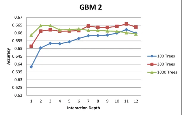
For the first model the highest accuracy achieved with interaction depth 5 and number of trees is 600. Same analysis conducted for the other three models and the behavior was similar. The following diagram illustrates the system behavior for the second GBM model. 0.61 0.615 0.62 0.625 0.63 0.635 0.64 0.645 0.65 0.655 1 2 3 4 5 6 7 8 9 10 11 12 A cc u rac y Interaction Depth

GBM 1

100 Trees 600 Trees 1000 Trees

(43)

33

The second GBM model had higher accuracy results at 300 trees with depth 11. The overfitting was very obvious in the case of 1000 trees where the accuracy dropped after three levels of depth. The third GBM model’s accuracy achieved its highest accuracy at 950 trees on three levels of depth. The overfitting occurred after the third level of depth. 0.62 0.625 0.63 0.635 0.64 0.645 0.65 0.655 0.66 0.665 0.67 1 2 3 4 5 6 7 8 9 10 11 12 A cc u rac y Interaction Depth

GBM 2

(44)

34

The fourth GBM model with the highest accuracy was achieved at 1000 trees with interaction depth 3. The results with 1000 trees were very close to the baseline results; however a slight increase in accuracy was achieved with 1000 trees.

0.62 0.625 0.63 0.635 0.64 0.645 0.65 0.655 0.66 0.665 1 2 3 4 5 6 7 8 9 10 11 12 A cc u rac y Interaction Depth

GBM 3

(45)

35

The results achieved for the four models were higher than the results from the baseline test. The table below compares the baseline test values with the achieved values.

Table 3 Comparing Old and New Results

Baseline model Results Difference

GBM Model

Trees Interaction Depth

Accuracy Trees Interaction Depth Accuracy 1 650 7 0.64687 600 5 0.64987 0.003 2 600 7 0.66352 300 11 0.6658 0.00228 3 600 7 0.65894 950 3 0.66138 0.00244 4 600 7 0.66207 1000 3 0.66461 0.00254 0.625 0.63 0.635 0.64 0.645 0.65 0.655 0.66 0.665 0.67 1 2 3 4 5 6 7 8 9 10 11 12 A cc u rac y Interaction Depth

GBM 4

(46)

36

Each model behaved similarly but with different results at the highest accuracy. A general appearance of the results from the first model on each run is represented in the following graph.

Figure 8 GBM 1 Results

From the graph above, for the same interaction depth, as the number of trees increased the accuracy increased. However, after the interaction depth of 7 the model tends to have overfitting which dropped the accuracy. For example, in cases such as 1000 trees and 100 trees at interaction depth 10 the accuracy of 100 trees was higher than 1000. The next graph illustrates the analysis for the second GBM model.

GBM 1

100 Trees 200 Trees 300 Trees 400 Trees 500 Trees 600 Trees 700 Trees 750 Trees 800 Trees 850 Trees 900 Trees 950 Trees 1000 Trees

(47)

37 Figure 9 GBM 2 Results

For the second model, the results were very close to each other with the same interaction depth; especially after 400 trees. Same as the previous graph, while moving forward the overfitting started to appear as the number of trees increased. Such as the case of 900 trees or 1000 trees compared to 200 trees or 300 trees. The next graph presents the behavior of the third GBM model.

0.62 0.625 0.63 0.635 0.64 0.645 0.65 0.655 0.66 0.665 0.67 1 2 3 4 5 6 7 8 9 10 11 12 A cc u rac y Interaction Depth

GBM 2

100 Trees 200 Trees 300 Trees 400 Trees 500 Trees 600 Trees 650 Trees 700 Trees 750 Trees 800 Trees 850 Trees 900 Trees 950 Trees 1000 Trees

(48)

In the graph above, for each tree the differences between the results were not large due to a change in input parameters. It is hard to tell from the graph above when the overfitting occurred. However, looking at the highest value recorded, at depth 3 and 950 interaction depth, one could conclude the overfitting occurred after this point which explains the compactness of results for trees less than 950.

GBM 3

100 200 300 400 500 600 650 700 750 800 850 900 950 1000

(49)

The graph above represents the forth model. The results were very similar to the third model in which higher accuracy at the larger number of trees with small values of interaction depth.

Summary

To summarize the findings, the shrinkage value tuned to 0.1 the number of trees and interaction depth tuned as the following table.

GBM 4

100 Trees 200 Trees 300 Trees 400 Trees 500 Trees 600 Trees 650 Trees 700 Trees 750 Trees 800 Trees 850 Trees 900 Trees 950 Trees 1000 Trees

(50)

40 Table 4 Results with Shrinkage 0.1

GBM model Number of Trees Interaction Depth

GBM 1 600 5

GBM 2 300 11

GBM 3 950 3

GBM 4 1000 3

The table above concluded from the previous graphs, the general behavior for the models was low accuracy at small values of interaction depth and number of trees. The accuracy got higher as moving forward with number of trees and interaction depth. The results starts to drop after a point where the overfitting starts to occur due to extensive learning from using higher values of interaction depth and trees. When large number of trees used less interaction depth needed to reach maximum value regarding that number of trees and the opposite for small number of trees.

(51)

41 CHAPTER V

SUMMARY, CONCLUSIONS, AND RECOMMENDATIONS Summary of the Research Problem,

Methods and Findings

The winner’s model of KDD Cup 2014 implemented a model using GBM and decision trees. The model consists of four GBM ensembles and one extra tree. Those models have parameters that affect the results which is the major component of the study. Since the problem presented in the competition is a data mining problem, CRISP

methodology followed to address and the study the stated problem with focus on evaluation phase. Due to resource limitation only the GBM models studied and tuned. Multi-way parameter sensitivity used to analyze the parameters for each model. The results indicated that the models can be tuned to achieve higher values of accuracy.

Conclusion and Implications

Sensitivity analysis was a very effective approach to study the behavior for each model independently to achieve higher accuracy. Although in total there are more than 600 runs and results to study; however it provides a practical justification for the parameter selection process to maximize the results. This is needed in a competitive environment, such as Kaggle.

The analysis shows that increasing the number of trees at a fixed value of

(52)

42

trees is higher than accuracy for 100 trees at interaction depths 2 or 3 for the first GBM. However, at some point increasing the number of trees did not increase the accuracy because the model starts to overfit the training data set. For example, in GBM 1 at interaction depth of 10, the accuracy of 300 trees was higher than that of 900 because the model started to overfit the data which validates first hypothesis H1.

The analysis shows that increasing interaction depth at a fixed number of trees increased the system accuracy. For instance, the accuracy for using interaction depth 2 is higher than accuracy for interaction depth 1 at 100 trees or 200 trees for the first GBM. However, at some point increasing the interaction depth did not increase the accuracy because the model starts to overfit the training data set. For instance, in GBM 1 at interaction depth of 6, the accuracy of 600 trees was higher than interaction depth 7 because the model starts to overfit at interaction depth of 6 which validate the second hypothesis H2.

It is noted from the analysis that there is a relation between overfitting, interaction depth and number of trees. As the number of trees increased less depth required to reach the maximum value. After the maximum point the GBM model starts to overfit the training data rather than increase the prediction accuracy. Therefore, using large number of trees with high interaction depth does not mean increasing accuracy. This relation was obvious from the results, the maximum accuracy achieved on either high number of trees such as 950 & 1000 in GBM 3 & 4 with low interaction depth or at low number of trees such as 300 in GBM 2 with high interaction depth. While in the first model the highest accuracy was achieved on 600 trees with interaction depth of 5 which is neither low nor

(53)

43

high and complies with the number of trees-depth ratio. This relation validates the third hypothesis H3.

Shrinkage value is a practical value depends on the machine and memory used. Although it is advised to set shrinkage between 0.01 and 0.001, it was noted from the analysis that at small values like 0.0001 lower accuracy recorded due to low memory usage; same thing happened with 0.001 and 0.01. A shrinkage value of 0.1 was the optimum value with respect to memory because of the decline in model’s accuracy after 0.1 which comply with the theory. This analysis endorses the fourth hypothesis H4. Table 5 Hypotheses Summary

Hypotheses

Variables

Number of Trees Interaction Depth Shrinkage

H1 True

H2 True

H3 Inverse relation Inverse relation

H4 True

Sensitivity analysis applied in this research optimized the GBM models’ results compared to what were used in the competition. However, the values in the competition were acceptable and lead to algorithm with high accuracy even though the selected values less than the optimized values.

(54)

44

Recommendations for Future Research

For future research, I recommend to study the extra tree model and combine the results with the results founded in this study by using more resources that enable the execution of extra tree model.

(55)

45 REFERENCES

Abbott, D. W. (1999). Combining models to improve classifier accuracy and robustness. Proceedings of Second International Conference on Information Fusion, 289-295.

Azevedo, Ana Isabel Rojão Lourenço. (2008). KDD, SEMMA and CRISP-DM: A parallel overview.

Bi, J., Sun, J., Wu, Y., Tennen, H., & Armeli, S. (2013). A machine learning approach to college drinking prediction and risk factor identification. ACM Transactions on Intelligent Systems and Technology (TIST), 4(4), 72.

Breierova, L., & Choudhari, M. (1996). An introduction to sensitivity analysis. Prepared for the MIT System Dynamics in Education Project,

Chapman, P., Clinton, J., Kerber, R., Khabaza, T., Reinartz, T., Shearer, C., & Wirth, R. (2000). CRISP-DM 1.0 step-by-step data mining guide.

Chaudhuri, S., Dayal, U., & Narasayya, V. (2011). An overview of business intelligence technology. Communications of the ACM, 54(8), 88-98.

Chen, Y., & Chen, Y. (2009). Combining incremental hidden markov model and adaboost algorithm for anomaly intrusion detection. Proceedings of the ACM SIGKDD Workshop on Cybersecurity and Intelligence Informatics, 3-9. Christopher Frey, H., & Patil, S. R. (2002). Identification and review of sensitivity

analysis methods. Risk Analysis, 22(3), 553-578.

Erskine, J. R., Peterson, G. L., Mullins, B. E., & Grimaila, M. R. (2010). Developing cyberspace data understanding: Using CRISP-DM for host-based IDS feature mining. Proceedings of the Sixth Annual Workshop on Cyber Security and Information Intelligence Research, 74.

Friedman, J. H. (2001). Greedy function approximation: A gradient boosting machine. Annals of Statistics, 1189-1232.

Friedman, J. H. (2002). Stochastic gradient boosting. Computational Statistics & Data Analysis, 38(4), 367-378.

(56)

46

Friedman, J., Hastie, T., & Tibshirani, R. (2000). Additive logistic regression: A statistical view of boosting (with discussion and a rejoinder by the authors). The Annals of Statistics, 28(2), 337-407.

Hamby, D. (1994). A review of techniques for parameter sensitivity analysis of

environmental models. Environmental Monitoring and Assessment, 32(2), 135-154. Harding, J., Shahbaz, M., & Kusiak, A. (2006). Data mining in manufacturing: A review.

Journal of Manufacturing Science and Engineering, 128(4), 969-976. Isukapalli, S. S. (1999). Uncertainty analysis of transport-transformation models. James, G., Witten, D., & Hastie, T. (2014). An introduction to statistical learning: With

applications in R.

Kaggle Inc. (2013). KDD cup 2013 - author-paper identification challenge (track 1). Retrieved from

https://www.kaggle.com/c/kdd-cup-2013-author-paper-identification-challenge

Kaggle Inc. (2014a). Attach submission - KDD cup 2014 - predicting excitement at DonorsChoose.org | kaggle. Retrieved from http://www.kaggle.com/c/kdd-cup-2014-predicting-excitement-at-donors-choose/submissions/attach

Kaggle Inc. (2014b). KDD cup 2014 - predicting excitement at DonorsChoose.org. Retrieved from http://www.kaggle.com/c/kdd-cup-2014-predicting-excitement-at-donors-choose

Kaggle Inc. (2014c). KDD cup 2014 - predicting excitement at DonorsChoose.org. Retrieved from http://www.kaggle.com/c/kdd-cup-2014-predicting-excitement-at-donors-choose/data

Kaggle Inc. (2014d, July,2014). KDD cup 2014 - predicting excitement at DonorsChoose.org. Retrieved from

http://www.kaggle.com/c/kdd-cup-2014- predicting-excitement-at-donors-choose/forums/t/9774/congrats-to-straya-nccu-and-adamaconguli/51183#post51183

Ruß, G., & Brenning, A. (2010). Data mining in precision agriculture: Management of spatial information. Computational intelligence for knowledge-based systems design (pp. 350-359) Springer.

StatSoft. (2009). Introduction to boosting trees for regression and classification. Retrieved from http://www.statsoft.com/Textbook/Boosting-Trees-Regression-Classification

(57)

47

Taylor, M. (2009). What is sensitivity analysis. Consortium YHE: University of York, , 1-8.

Thearling, K. (1999). An introduction to data mining.

Whitepaper.Http://www3.Shore.Net/~ kht/dmwhite/dmwhite.Htm,

Wu, X., Kumar, V., Quinlan, J. R., Ghosh, J., Yang, Q., Motoda, H., . . . Philip, S. Y. (2008). Top 10 algorithms in data mining. Knowledge and Information Systems, 14(1), 1-37.

Yao, J. (2003). Sensitivity analysis for data mining. Fuzzy Information Processing Society, 2003. NAFIPS 2003. 22nd International Conference of the North American, 272-277.

(58)

48 APPENDIX A DATA DESCRIPTION

Outcome Table

is_exciting - ground truth of whether a project is exciting from business perspective

at_least_1_teacher_referred_donor - teacher referred = donor donated because teacher

shared a link or publicized their page

fully_funded - project was successfully completed

at_least_1_green_donation - a green donation is a donation made with credit card, PayPal, Amazon or check

great_chat - project has a comment thread with greater than average unique comments

three_or_more_non_teacher_referred_donors - non-teacher referred is a donor that

landed on the site by means other than a teacher referral link/page

one_non_teacher_referred_donor_giving_100_plus - see above

donation_from_thoughtful_donor - a curated list of ~15 donors that are power donors

and picky choosers (we trust them selecting great projects)

great_messages_proportion - how great_chat is calculated. proportion of comments on

the project page that are unique. If > avg (currently 62%) then great_chat = True

(59)

49

non_teacher_referred_count - number of donors that were non-teacher referred (see

above)

Projects Table

projectid - project's unique identifier

teacher_acctid - teacher's unique identifier (teacher that created a project)

schoolid - school's unique identifier (school where teacher works)

school_ncesid - public National Center for Ed Statistics id

school_latitude school_longitude school_city school_state school_zip school_metro school_district school_county

school_charter - whether a public charter school or not (no private schools in the dataset)

school_magnet - whether a public magnet school or not

school_year_round - whether a public year round school or not

school_nlns - whether a public nlns school or not

school_kipp - whether a public kipp school or not

school_charter_ready_promise - whether a public ready promise school or not

(60)

50

teacher_teach_for_america - Teach for America or not

teacher_ny_teaching_fellow - New York teaching fellow or not

primary_focus_subject - main subject for which project materials are intended

primary_focus_area - main subject area for which project materials are intended

secondary_focus_subject - secondary subject

secondary_focus_area - secondary subject area

resource_type - main type of resources requested by a project

poverty_level - school's poverty level. highest: 65%+ free of reduced lunch high: 40-64%

moderate: 10-39% low: 0-9%

grade_level - grade level for which project materials are intended

fulfillment_labor_materials - cost of fulfillment

total_price_excluding_optional_support - project cost excluding optional tip that donors give to DonorsChoose.org while funding a project

total_price_including_optional_support - see above

students_reached - number of students impacted by a project (if funded)

eligible_double_your_impact_match - project was eligible for a 50% off offer by a

corporate partner (logo appears on a project, like Starbucks or Disney)

eligible_almost_home_match - project was eligible for a $100 boost offer by a corporate partner

(61)

51

Donations Table

donationid - unique donation identifier

projectid - unique project identifier (project that received the donation)

donor_acctid - unique donor identifier (donor that made a donation)

donor_city donor_state donor_zip

is_teacher_acct - donor is also a teacher

donation_timestamp

donation_to_project - amount to project, excluding optional support (tip)

donation_optional_support - amount of optional support

donation_total - donated amount

dollar_amount - donated amount in US dollars

donation_included_optional_support - whether optional support (tip) was included for

DonorsChoose.org

payment_method - what card/payment option was used

payment_included_acct_credit - whether a portion of a donation used account credits

redemption

payment_included_campaign_gift_card - whether a portion of a donation included

corporate sponsored giftcard

payment_included_web_purchased_gift_card - whether a portion of a donation