1. Project Summary Title Primary Contact Recipient Institution Partners: overall goal

1. Project Summary

Title: Using ocean data assimilation to incorporate environmental variability into sardine and squid assessments

Primary Contact: Dr. Arthur J. Miller, Climate Research Division, Scripps Institution of Oceanography, UCSD, La Jolla, CA 92093-0224 858-534-8033, ajmiller@ucsd.edu

Recipient Institution: Scripps Institution of Oceanography, UCSD, La Jolla, CA 92093 Partners: Dr. Sam McClatchie, Dr. Kevin Hill, NOAA, NMFS, SWFSC

Prof William Hamner, Dr. Lou Zeidberg, UCLA

Prof David Checkley, Dr. Bruce Cornuelle, Prof John McGowan, Dr. Tony Koslow, Dr. Guillermo Auad, Dr. Ibrahim Hoteit, SIO/UCSD

Dr. Tim Baumgartner, CICESE, Ensenada, Mexico

Sardine and market squid are important fisheries in the California Current System (CCS) from Mexico to Canada as a commercial fishery whose stocks are actively managed and as forage fish for other important commercial stocks such as tuna. The current sardine and squid stock assessment assumes that spatial variability is not a major influence. In fact, this assessment is unique by including the sea-surface temperature (SST) time series at Scripps Pier in La Jolla, CA, in the final management decision. Although the Scripps pier SST is broadly coherent with large-scale SST all along the coast on climatic timescales, there is also tremendous mesoscale and interannual spatiotemporal temperature variability throughout the CCS, as well as in other biologically relevant fields, such as upwelling, squirts, streamers and eddies. Local temperature, along with forage and predation are known to affect the growth and condition of sardine and squid. Since both move yearly inshore and offshore along the entire coast of the U.S., the spatial components of temperature and forage on stock recruitment are likely to be important.

We therefore propose to investigate whether this spatial component can be quantified using IOOS (SCCOOS and CeNCOOS) datasets in the CCS, supplemented with other observations. Our overall goal is to develop a coupled ecological and hydrologic model for assessing and predicting the physical oceanographic influences on sardine and squid stocks using both the Regional Integrated Ocean Observing System datasets in the California Current System and NOAA’s Fisheries and CalCOFI data. The resulting forecast will be presented to sardine and squid stock managers and scientists for consideration in the catch quotas for these species.

The project will include extensive analysis of the various IOOS data using sophisticated ocean data assimilation tools. We will develop spatial models to relate sardine larvae and squid paralarvae to objectively selected environmental variables from the assimilated ocean physical fields. We aim to characterize the ocean (pelagic) habitat suitable for sardine production and use assimilated ocean fields to identify the physical processes that influence development of this habitat. We will also compare the assimilated ocean fields to two aspects of squid biology, hatchling abundance and egg bed habitat, and to then compare to fishery landings data. We will also establish the relationships between variations in the abundance of larval fish species and the abundance of functional groups of predators and prey over time and space as diagnosed in the assimilated ocean physical fields and examine the physical/chemical oceanographic variables associated with the correlations that we expect to find.

This research bridges NOAA NMFS-SWFSC scientists with UCSD and UCLA researchers, and unites physical oceanographers with fisheries biologists to develop an integrated analysis of physical-biological interactions with applications in fisheries management. Benefits include: Enhancing the value of environmental data incorporated into decision rules used in the sardine

assessment; assessing the predictability of fisheries for management forecasts; providing experimental forecasts one year in advance predicting favorable or unfavorable recruitment of sardine and squid; generating a more mechanistic understanding of the environmental forcing that contributes to inter-annual fluctuations in the abundance of sardine and squid; producing a better understanding of key forage species for sardine and squid; educating young scientists. The primary user of this work will be the Coastal Pelagic Species Management Team and Scientific and Statistical Committee of the Pacific Marine Fisheries Management Council who review scientific advice on sardine harvests for the entire West Coast.

2. Background

Sardine and market squid are important fisheries in the California Current System (CCS) from Mexico to Canada as a commercial fishery whose stocks are actively managed and as forage fish for other important commercial stocks such as tuna. The current sardine and squid stock assessment assumes that spatial variability is not a major influence. In fact, this assessment is unique by including the sea-surface temperature (SST) time series at Scripps Pier in La Jolla, CA into the final management decision. Although the Scripps pier SST is broadly coherent with large-scale SST all along the West Coast on climatic timescales (McGowan et al., 1998; Reiss, 2007), there is also tremendous mesoscale and interannual spatiotemporal temperature variability throughout the CCS, as well as in other biologically relevant fields, such as upwelling, squirts, and eddies (Hickey, 1998; Mendelssohn et al., 2004; Miller et al., 1999; Roughan, 2005).

Local temperature, along with forage and predation are known to affect the growth and condition of both sardine and squid. Survival and mortality is also influenced by advective loss, or by retention in eddies, which may be beneficial or deleterious to survival depending on

whether eddies are upwelling or downwelling favorable (Logerwell and Smith, 2001). Since both move yearly inshore and offshore along the entire coast of the U.S., the spatial components of temperature and forage on stock recruitment are likely to be important.

We therefore propose to investigate whether this spatial component can be quantified using IOOS (SCCOOS and CeNCOOS) datasets in the CCS, supplemented with other in situ and remote observations, with the goal of improving the current method for incorporating

environmental variability into the Pacific Fisheries Management Council’s sardine and squid assessments. This research bridges NOAA NMFS-SWFSC scientists with UCSD and UCLA researchers, and unites physical oceanographers with fisheries biologists to develop an integrated analysis of physical-biological interactions with applications in fisheries management.

Pacific Sardines

Pacific sardine (Sardinops sagax) historically supported the largest commercial fishery in the state of California. Beginning in the late 1940s and continuing into the 1960s the sardine

population of the California Current suffered a dramatic decline from almost 4 million metric tons to less than 10,000 tons during a period of cooling of the coastal ocean (Fig. 1). The sardines disappeared from their traditional fishing grounds precipitating the collapse of the sardine fishing and processing industries and impacting local economies in the region. A recovery in the population could finally be detected in the late 1980s (Fig. 1).

The public blamed poor management and overfishing for the decline while fishermen blamed it on climatic changes. Both may be partially correct. Changes in sardine biomass are thought to reflect variability in the natural environment, but the mechanisms relating physical changes to sardine production remain obscure (Lluch-Belda et al., 1989; Chavez et al., 2003). Several

studies (e.g., Roemmich & McGowan, 1995) have shown that climatic variations are almost certainly involved, and decadal variability in populations is natural (Baumgartner et al., 1992).

Investigation of ecosystem-based hypotheses relating climate changes to sardine production has been restricted by the lack of time-series measurements of multiple environmental variables (Jacobson and MacCall, 1995). These existing hypotheses do not provide the understanding necessary to predict how fisheries will respond under future climate conditions. Now, with the accumulation of atmospheric, hydrographic, and biological data collected by satellites, ships, moorings, and coastal stations, examination of more mechanistic hypotheses is possible.

The highest mortality in the sardine population occurs during the egg and larval, pre-recruit, life stages (Smith et al., 2001). Survival during these stages is the most significant factor

influencing total population biomass and requires suitable habitat and prey field. This prey field is limited to a certain planktonic size range determined by the mouth-gape diameter of the sardine during the larval stage and the morphology of the branchial sieve used by filter-feeding juveniles and adult fish (Arthur, 1976; King and MacLeod, 1976). Dietary and morphological analyses of sardine inhabiting the Benguela Current off the west coast of Africa indicate that adults prey most efficiently on small size classes of plankton. Field and laboratory studies have shown that adult sardine consume small (<1.2 mm total length) prey and their fine-mesh

branchial sieve is capable of retaining prey items as small as 0.01 mm (van der Lingen, 2006). Currently, little is known concerning the relationships between plankton size and pre-recruit sardine diet in the CCS. It is hypothesized that the relationship between physical variability and sardine production in the CCS may be mediated by the variability in individual plankton sizes resulting from different rates of upwelling and nutrient supply (Rykaczewski & Checkley, 2007).

The rate of nutrient supply in an ecosystem influences the size and amount of plankton production. Nutrient uptake kinetics favor smaller cells (with higher surface-area-to-volume

Figure 1. (top) Time-series of sardine biomass estimates using different methods. Data are from Barnes et al. (1992) and Lo et al. (2005). Data are centered (by dividing by the mean of each series) and scaled (by dividing the centered values by the root mean squared variance). Although there is no consistent biomass series, the relative trends in these indices show the no-fishery period from the 1960’s to the late 1980’s and subsequent

indications of upward trend, but with high variability. (bottom) Pacific Decadal Oscillation index (Mantua et al., 1997), showing the transition from a cool to a warm “regime” for comparison with trends in the sardine time series.

ratios) in nutrient-limited environments where vertical velocities in the water column are small (Morel et al., 1991). The increased nutrient concentrations present in vigorously upwelling waters lessen the diffusive advantage of small cells, allowing populations of large cells with lower surface-area-to-volume ratios to develop. Given that prey size correlates positively with predator size (Landry, 1977), larger zooplankters are expected in areas with larger

phytoplankters and higher upwelling rates. SCCOOS provides size-structured estimates of phytoplankton biomass, while zooplankton sizes have been estimated using net samples and the laser optical plankton counter during CalCOFI and Long-Term Ecological Research cruises in the CCS. The status and role of larval fish in the zooplankton community, however, is not well understood (McGowan and Miller, 1980), although they are certainly rare relative to species of copepods, chaetognaths, thaliacean, and others. This implies that each individual larval fish is surrounded by many potential competitors or predators. Their survivorship depends on the intensity of this interaction between functional groups, which is not well understood although changes in absolute and relative abundance have been documented (Fleminger et al., l974; McGowan et al., 1998; Lavaniegos and Ohman, 2003)

Interannual changes in ocean climate (temperature, mesoscale eddy statistics, transport properties, upwelling, etc.) may play an important role in regulating the population size by affecting the survival of juvenile sardines (less than 1 year of age). A statistical model of the relationship between annual sardine reproductive success and interannual variability in ocean climate over the period 1984-2005 (Fig. 2; Baumgartner et al., 2007) indicates a high sensitivity to offshore Ekman transport and to the SST pattern of the PDO. The study by Logerwell & Smith (2001) indicates a link between mesoscale eddy statistics and sardine recruitment off California suggesting that eddies act as incubators for fry and pre-recruitment adults. Food for these sardines is thought to be locally produced in the Southern California Bight (SCB), and then moved offshore and sequestered in eddies forming in the CCS. Baumgartner et al. (2007) propose that zooplankton food for the sardines is generated principally along the central

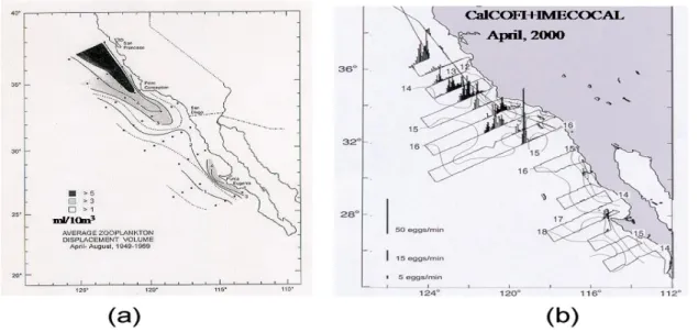
California coast, and farther north, in the zone of coastal upwelling, and advected offshore to be concentrated in the front between the upwelled water and water transported south by the CCS. The southern limit of the more abundant zooplankton stocks occurs along a significant oceanic frontal feature known as the Ensenada Front. The result of averaging of these processes over 20 years is shown in Fig. 3 as the distribution of mean zooplankton biomass for April-August for

Figure 2. Comparison of observed values of reproductive success of the Pacific sardine, Ln[R/S] (from Hill et al., 2006), with predicted values obtained from multi-regression model with nine environmental variables (indices of PDO-SST, Ekman pumping, coastal upwelling and zooplankton volume at various lags) acting over successive life stages. Model explains 80% of the variance in the reproductive success (R2=0.80; p<0.004). Baumgartner et al. (2007).

the years 1949-1969. This distribution would be sensitive to climatic changes that affect the eddy statistics and flow associated with the CCS and SCB.

California Market Squid

The California market squid, Loligo opalescens has become the largest commercial fishery in Calilifornia in the last dozen years, in terms of both tonnage and economic value (Zeidberg et al. 2006). Proper management of the market squid fishery is important not only for human

consumption, but also the birds, fish, and marine mammals that utilize this organism as a key forage species. In California, market squid are the most important nearshore species for the transfer of energy from zooplankton to marine mammals and birds. Squid have a short, approximately one year, life span and their growth rate is inversely correlated to temperature (Reiss et al. 2004). As such they are uniquely positioned for the purpose of modeling the life history of a key forage species from the perspective of bottom-up climate forcing.

Recent studies have enhanced the understanding of the life history of Loligo opalescens. Female squid insert egg capsules containing 100-200 embryos into sandy bottom substrates (Okutani and McGowan 1969, Zeidberg et al. 2004). Eggs are left unattended and develop over the next several weeks (McGowan 1954) and they are gently ventilated by surface wave surge. Upon hatching, squid paralarvae are found at a depth of 30m by day and 15m at night, this diel migration may serve to aggregate them for weeks at tidal-neritic fronts 1-3km from shore (Zeidberg and Hamner 2002). Juvenile L. opalescens begin to school at 15mm mantle length (ML) or 2 months age (Hurley 1978, Butler et al. 1999) and occur on the shelf just off the bottom by day and throughout the water column at night (Zeidberg 2004). As they reach 55mm ML the squid move off the slope (Zeidberg 2004) and occur down to 500 m by day and at the surface at night (Hunt 1996). Adult squid return to the shelf waters to spawn at an age of 4-10 months in

Figure 3. (a) Averaged distributions of zooplankton abundance sampled by CalCOFI during annual periods of April-August from 1949 through 1969, based on measurements of relative displacement volume of wet biomass from standard oblique net tows down to 140m depth (redrawn from Chelton et al., 1982); (b) Distribution and abundance of sardine eggs off California and Baja California during April, 2000 plotted over surface isotherms. The egg data were collected with Continuous Underway Fish Egg pumping Systems (CUFES, Checkley et al., 2000) on simultaneous CalCOFI and IMECOCAL cruises off California and Baja California. Relative egg abundances are plotted as vertical bars expressing eggs per minute of flow from the egg pump along the ship survey tracklines.

waters of 15-200m. Individual squid size is related to El Niño/Southern Oscillation (ENSO) events, with smaller squids of the same age migrating onto spawning grounds during El Niño, and larger squid reproducing in La Niña (Jackson and Domeier 2003). Monthly growth rate is inversely proportional to sea surface temperature (Reiss et al. 2004).

Squid are difficult to catch in nets. Fisheries target spawning aggregations because individuals are otherwise distracted. Juveniles and non-spawning adults often manage to slip right through nets (Mais 1974). Eggs occur patchily in murky depths and require massive hours of ROV time to properly catalogue presence or absence. Although there have been recent advances in acoustic egg counting techniques that can identify squid egg mops in 40m deep waters (Foote et al. 2006), this acoustic technique has not been field tested in waters deeper than 40m and would be very expensive in areas with vast spawning grounds, like Southern California. Developing environmental proxies for squid recruitment is a useful way forward towards more effective assessment of squid.

IOOS Datasets

The components of IOOS in the California Current System include SCCOOS (Southern California Coastal Ocean Observing System: http://www.sccoos.org/) and CeNCOOS (Central and Northern California Ocean Observing System: http://www.cencoos.org/). Many disparate environmental variables are collected with a wide variety of spatial and temporal sampling patterns. These include hydrographic profiles, upper-ocean ADCP currents, chlorophyll and nitrate from ships in the California Cooperative Oceanic Fisheries Investigations (CalCOFI); surface currents from CODAR stations; T-S profiles from gliders and profiling floats; satellite observations of sea level, SST, ocean color and surface winds; as well as many other variables.

The extensive IOOS datasets in the CCS provide a unique opportunity to combine ocean data assimilation techniques, which blend observations with dynamics, to better understand the environmental conditions that may be affecting populations of sardine and squid.

3. Goals and Objectives

Our overall goal is to develop a coupled ecological and hydrologic model for assessing and predicting the physical oceanographic influences on sardine and squid stocks using both the Regional Integrated Ocean Observing System datasets in the California Current System and NOAA’s Fisheries and CalCOFI data. The resulting forecast will be presented to the sardine and squid stock managers and scientists for consideration in the catch quotas for these species.

The project will include extensive analysis of the various IOOS data using sophisticated ocean data assimilation tools. For example, detailed oceanic temperature fields will be combined with statistical analysis of the spatial and temporal observed distributions of sardine and squid eggs, larvae, recruits and populations, to develop a better understanding of the environmental controls on these important marine populations.

We will develop spatial models to relate sardine larvae and squid paralarvae to objectively selected environmental variables from the assimilated ocean physical fields, including

temperature, salinity, mixed layer depth, currents, eddies, fronts, and water column stability, plus other relevant biological variables such as chlorophyll and zooplankton biomass. The selected environmental variables will be supplemented with measures of sardine and squid condition, derived from length-weight regressions of larvae and of adults.

We aim to characterize the ocean (pelagic) habitat suitable for sardine production and use assimilated ocean fields to identify the physical processes that influence development of this habitat. The real puzzle that fisheries oceanographers have struggled with over the past several

decades is why sardine grow in abundance during warm periods associated with anomalously low upwelling and low production along the coast. We are proposing that it is not raw plankton production that is important for sardine survival, but production of suitable prey, i.e. plankton within a certain size range, specifically smaller plankton sizes resulting from weaker upwelling driven by wind-stress curl. Plankton community structure is a habitat characteristic that can be accurately estimated by examination of physical environmental variables.

We will also compare the assimilated ocean fields to two aspects of squid biology, hatchling abundance and egg bed habitat, and to then compare to fishery landings data. Squid prerecruit indices will be derived from the distribution and abundance of paralarvae.

We will also establish the relationships between variations in the abundance of larval fish species and the abundance of functional groups of predators and prey over time and space as diagnosed in the assimilated ocean physical fields and examine the physical/chemical

oceanographic variables associated with the correlations that we expect to find. 4. Approach

We propose to study the influence of physical oceanography on the populations of sardine and squid by selecting key El Niño and La Niña time periods (which are representative of environmental extremes) for intensive analysis, comparison, and contrast to typical conditions. First, the physical oceanographic state during the key years will be studied using sophisticated ocean data assimilation tools of the Regional Ocean Modeling System (ROMS). Second, the biological observations will be related to the time-evolving physical state using statistical

models. Third, the predictive capability of the physical-biological system will be evaluated using independent years of data. In all three steps, the SWFSC stock assessment scientist will advise on applicability of the predictions. At the end of the project, the system will be delivered to stock assessment managers through the SWFSC scientists.

Ocean Modeling and Data Assimilation Framework

The basic strategy is as follows. First, the physical ocean observations will be simulated for the chosen time period by running the physical ocean model in the CCS domain with observed atmospheric forcing. Then the model initial and boundary conditions and surface forcing will be adjusted using 4D variational assimilation (4DVar) procedures to improve the model fit to the data. Then the simulation will be diagnosed to identify the relevant physical processes for

biological production during the key time intervals. Additional diagnostic tools using the tangent linear and adjoint models will allow novel views of the sources of upwelled water and the

sensitivity of different regions to surface forcing and initial conditions.

We will use ROMS, a state-of-the-art, free-surface, hydrostatic primitive equation ocean circulation model developed at Rutgers University and UCLA with a user community of over 600 scientists worldwide. ROMS is a terrain-following, finite difference model with the following advanced features: sustained performance on parallel-computing platforms (MPI); high-order, weakly dissipative algorithms for tracer advection; unified treatment of surface and bottom boundary layers based on KPP algorithms; and an integrated set of procedures for data assimilation. Numerical details can be found in Haidvogel et al. (2000), Moore et al. (2004), Shchepetkin and McWilliams (2004) and Haidvogel et al. (2007). ROMS also has a suite of Generalized Stability Analysis tools (Moore et al., 2004; Moore et al., 2007), which allow the quantitative assessment of sensitivities of model solutions to various parameters.

Data assimilation of key time intervals, typically spanning one-to-three months during spawning season, will be achieved using the Inverse Regional Ocean Modeling System

(IROMS), a 4D-variational data assimilation system for high-resolution basin-wide and coastal oceanic flows (Di Lorenzo et al., 2007). IROMS makes use of the recently developed

perturbation tangent linear (TL), representer tangent linear (REP) and adjoint (AD) models of ROMS to implement a “representer”-based generalized inverse modeling system. The TL, REP and AD models are used as stand-alone sub-models within the Inverse Ocean Modeling (IOM) system described in Chua and Bennett (2001). It allows the assimilation of many observation types, using an iterative algorithm to solve nonlinear problems (Muccino et al. 2007).

The assimilation can be performed either under the perfect model assumption (strong constraints) or by also allowing errors in the model dynamics (weak constraints). For the weak constraint case the TL, REP and AD models are modified to include additional (non-physical) forcing terms on the right hand side of the model equations. These terms are needed to account for errors in the model dynamics. Posterior error statistics, term balances and array assessment are computed using separate diagnostic tools provided by the IOM. Since we wish to diagnose physical balances during the key time periods, we plan to use a strong constraints approach in our assimilations of the data (over 1-to-3 month fitting intervals suitable for mesoscale eddies).

IROMS has been tested by Di Lorenzo et al. (2007) in an idealized 3D double gyre circulation and in a realistic application for the geometry and bathymetry of the Southern California Bight, a region characterized by strong mesoscale eddy variability. Synthetic data for sea surface height, upper ocean (0-500m) temperatures, salinities and currents were assimilated over a period of 10 days. The model first-guess was initialized using climatological conditions. The assimilation solution for the strong constraint experiment significantly improved the model fit to the data and improves the model fields also at locations where observations are not

assimilated. Forecast skill of the fit exceeded the skill of persistence.

An application of the assimilation framework to real data was conducted in May 2006. We performed a 1-month forecast from April 2006 CalCOFI initial conditions that were used to guide the follow-up May 2006 LTER process-study cruise. The model forecast was done in real time and posted on the web (http://www.o3d.org/web/CalCOFI/april2006/) and successfully used by shipboard scientists to anticipate frontal locations and movements during the LTER cruise. IOOS Modeling and Data Assimilation Applications

In support of the sardine and squid analyses, we will execute data assimilation fits for each of the key time periods. These fits will attempt to reconstruct the mesoscale circulation observed during CalCOFI cruises using in situ temperature and salinity data, along with ADCP upper-ocean currents, satellite altimetric estimates of sea level, satellite observations of SST, mooring currents, and whatever other data types are available in the IOOS.

The procedure involves generating a first-guess (prior) initial state for the model, by using all the data in an objective analysis and mapping it to the model grid. First-guess (prior) surface forcing will come from the downscaled NCEP wind stresses and heat fluxes (Kanamaru and Kanamitsu, 2007). First-guess boundary conditions will come from the North Pacific ROMS grid hindcasts (available from our other research projects). The data assimilation grid will cover most of the CCS region, including the SCB. The model will then be run forward through the data assimilation time period, which will span the roughly one to three months (depending on the duration of the cruises), to generate the first-guess of the 4D evolution of the flows.

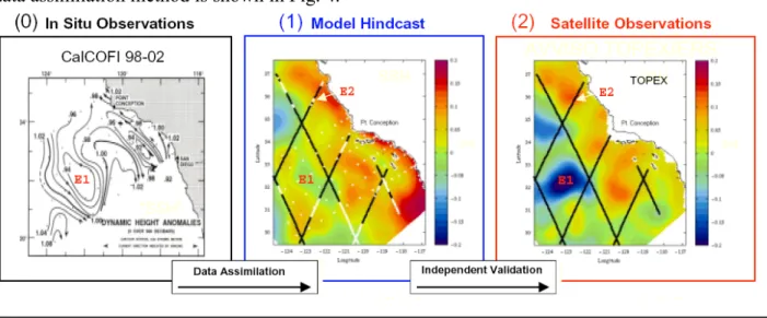
We will then use the IROMS representer method to correct the initial conditions, surface forcing and boundary conditions of the runs, in an iterative procedure according to the IROMS formalism to minimize the mismatch between the observations and the model fields. The final result will be a dynamically consistent 4D representation of the mesoscale flows observed over the California Current during the key time periods. An example of a fit using a different inverse data assimilation method is shown in Fig. 4.

We will use these fits to diagnose the processes that control the observed physical variability that determines the nutrient transport and mixing properties observed in the surveys. Cross-shelf transports can be evaluated by releasing model float to compute Lagrangian particle statistics over the shelf-slope system. Passive tracer fields can be allowed to advect, mix, and diffuse in initial-condition experiments to determine the efficiency of horizontal and vertical mixing via eddies, mean flows, and other anomalous flows. Mixed-layer depths will be evaluated for the model runs and the in situ observations to determine what controls the variability in the fits. These biologically relevant effects will be studied as the seasonal cycle evolves through the spring bloom and spawning seasons to test various biological hypotheses. The fits can then be used to better understand the physical variations that may be controlling the biological

observations. The fits will also be freely available to the IOOS community scientists who may wish to drive ecosystem models or use them in others ways.

Using the Generalized Stability Analysis Tools, we will compute the sensitivities of the flows in the CCS to atmospheric forcing – winds, air temperature, short wave radiation and remote oceanic flows (Moore et al., 2007). This will be an important diagnostic tool for these analyses of historical surveys. For example, Moore et al. (2007) execute a sensitivity calculation using the adjoint model of ROMS from which we were able to isolate the primary controls of the physical and biological circulations in the CCS.

Sardine and Squid Diagnostics

We will develop spatial models to relate survival indices of sardine larvae and squid paralarvae to ROMS-assimilated physical oceanographic variables, including temperature, salinity, velocity, upwelling, mixed layer depth, water column stability and observed chlorophyll and zooplankton biomass. There are no spatially related estimates of sardine recruitment, so we

Figure 4. Example of an inverse method fit using the ROMS for non-synoptic CalCOFI observations from February 1998. (0) CalCOFI dynamic height anomalies, (1) ROMS model simulations of the monthly mean sea level of the fit, (2) independent observations of sea level observed by TOPEX altimetry. Di Lorenzo et al. (2004).

will use larval survival to estimate abundance and distribution of prerecruit juvenile sardines. Squid prerecruit indices will be derived from the distribution and abundance of paralarvae. For certain nearshore sites, squid prerecruit indices will be extended back to 1981, the beginning of the modern fishery statistics, to examine impacts of El Nino events and decadal environmental variability on the abundance and distribution of squid paralarvae and adult landings data. Spatially Explicit Statistical Modeling

Statistical modeling will be used to supplement the data assimilation modeling by explicitly linking the environmental variables to the recruitment proxys for sardine and squid. We will investigate the effect of spatial scale on the distribution and abundance of sardine larvae and squid paralarvae and explanatory environmental variables using principal coordinate

neighborhood matrices (PCNM) (Borcard & Legendre 2002, Borcard et al. 2004). In contrast to methods that use polynomial fitting of spatial trend surfaces, the PCNM method starts with the fine rather than the broad scale. It has a superficial resemblance to Fourier analysis, but can be used on unevenly spaced data, and covers the full range of scales. Explanatory variables for regression analysis are initially derived from the spatial locations alone. To do this the

neighborhood distances between stations are expressed as truncated positive eigenvectors that are then clustered using principal coordinates analysis. The principal coordinates produced are a series of sinusoidal functions with different periods representing large to small scales. These principal coordinates can be used as explanatory variables when regressed against the dependent variable (in our case larval densities). Rather than using all of the principal coordinates in a multiple regression, a more parsimonious model is obtained by thinning those principal coordinates that do not meet a specified level of one-tailed significance in the multiple

regressions. The remaining significant principal coordinates are often clumped, and it is these clumps that define the broad-scale (long-period principal coordinates), mid-scale, or fine scale sub-models (short-period principal coordinates). The sub-models are obtained from multiple linear regressions using a clumped subset of the principal coordinates that have rather similar periods, and so represent rather similar spatial scales. The predicted values from these multiple regressions form a spatial sub-model (of larval distributions in our study) at each of the broad, mid and fine scales. These predicted values can then be regressed against the environmental variables in a second multiple linear regression to determine which of the environmental variables have significant effects on the distribution of the dependent variable in the spatial model at each scale (predicted densities of larvae). Although we refer to a linear regression here, non-linear approaches might well explain more of the variance, and will also be used. Each submodel can be plotted for each variable to determine if there are common spatial distributions between recruits and the environmental variables. The final result is a regression relationship that can be tested for statistical significance.

Squid-specific Analyses

Currently there are no fisheries independent (net tows) data for Loligo opalescens. Instead, the majority of the squid biomass data comes from fisheries landings data from purse seine vessels that capture adults that have aggregated from foraging slope waters to the shelf to spawn. Squid eggs are hard to find as they are benthic and patchy in California’s murky shelf waters (20-200m). Squid adults and juveniles are too fast to be captured with most plankton nets. So squid paralarvae are the best stage of the lifecycle for scientific enumeration.

Squid paralarvae occur in small numbers in CalCOFI zooplankton samples (especially nearshore sites) and have been enumerated from Manta tows back to 1981 by SWFSC staff.

However, the response of the squid population to the regime shift of 1976-77 as well as earlier climatic variability is not known. Expanding the time series back in time will greatly enhance our historical perspective on this population and our ability to relate population change to climate variability. For 2000-03, nearshore sampling of paralarvae will be compared to CalCOFI’s.

Existing data will be used to develop the spatial model. Because long time series are available they will be divided into a development subset and a test subset (Myers 1998). The spatial model will be derived from the development subset, including the seasonal data (rather than aggregating data into annually averaged dataset). The models derived from the development subset will be tested using the test subset, and a goodness of fit parameter estimated.

In developing the model, there is a wide range of possible explanatory variables.

Incorporating too many explanatory variables may detect significant effects by chance alone (Francis 2006). To reduce the possibility of this happening, we will apply an objective “test, remove one, and retest” procedure in order to select the most parsimonious set of explanatory variables. In addition to objectively selecting environmental variables we will also test if biologically sensible lag periods improve model fits (for short lags, especially for squid).

Squid paralarvae have been captured in nets (Okutani and McGowan 1969, Zeidberg and Hamner 2002, and Reiss et al. 2004) and provide a fishery independent sample of the population. Comparison of paralarvae to physical oceanography has provided correlative relationship

inversely proportional to temperature (Reiss et al. 2004) and El Niño (Zeidberg et al. 2006). Paralarvae occur from 15-30m depth (Zeidberg and Hamner 2002) and thus the bongo tow of the CalCOFI dataset is ideal for analysis. Reiss et al. (2004) utilized manta tow data which only surveys the upper 0.5m. Therefore we propose to compare CalCOFI bongo tow data to a variety of physical oceanography parameters from the CalCOFI data assimilation fits, including SST, mixed layer depth, salinity and density along with other observed variables including oxygen, nutrient levels, and zooplankton volume. Also we will compare fishery and non-fishery estimates of squid to assimilated SST, satellite ocean color, PFEG upwelling index, NINO-3 ENSO index, and PDO index. Samples have been sorted back to 1998, and we propose to sort all samples for the nearshore stations 83.51 and 83.43 back to 1981. Comparisons of these paralarvae indexes will be made to fisheries landings and to those of other surveys (Zeidberg et al. 2006).

We will attempt to model the ideal parameters of squid egg laying habitat. It is well known that fishermen are catching squid where they have massed together for the purpose of laying eggs. We will compare California Department of Fish and Game (CDFG) landings data to bathymetry data (SCCOOS and CenCOOS) to understand how spawning aggregations are confounded by depth and substrate. Seasonality of the optimal spawning grounds will then be determined by comparing landings data from CDFG to temperature depth data from assimilated CalCOFI cruises. Once these parameters of existing data are determined, attempts will be made to predict spawning habitats from temperature data 3-24 months prior.

Sardine-specific Observations

Sardine juveniles will be collected from commercial boats based in San Diego during summer and fall when pre-recruit sardine are abundant. Individuals will be preserved

immediately on deck to prevent continued digestion of prey items. Stomachs and gill rakers will be dissected in the laboratory to examine sardine diet and feeding morphology. Prey items will be examined microscopically, and the relative importance of each major prey type will be assessed based on total abundance and nutritional content. In addition, the spacing, length, and morphology of sardine gill rakers will be examined to estimate the filtering efficiency of the

branchial sieve used in feeding. These analyses will allow characterization of the species niche and identify which plankton types and sizes will promote survival of sardine pre-recruits.

The sizes of phytoplankton and zooplankton have been measured using size-fractionated filtration and a laser optical plankton counter during the partnership between CalCOFI,

SCCOOS, and the NSF-funded Long-Term Ecological Research (LTER-CCE) Program in the CCS since 2004. We will use these data to estimate the slope and intercept from the size-abundance spectrum for plankton (Platt and Denman, 1978). Spatial and temporal variability in these characteristics of the plankton community will be compared with concurrently measured physical conditions to establish relationships between the plankton type and physical conditions. Using these relationships, remotely sensed variables will be used to generate continuous

estimates of the plankton community throughout the year. Data gathered from satellite scatterometers and moored anemometers will be used to measure wind stress and wind-stress curl to estimate the vertical velocities of upwelling processes. Changes in sea-surface height and temperature will be measured using satellite altimeters and radiometers.

With a mechanistic understanding of how physical changes in the environment may influence sardine recruitment, the relevant physical-biological interactions will be integrated into the ROMS physical ocean model. Using this coupled, ecosystem-based model, we will better understand the spatial and temporal dynamics of the sardine population.

Functional Group Diagnostics

We will address the high temporal and spatial variability of larval survivorship by examining the time-space relationships between larval abundance and size frequencies versus the abundance of functional groups of their competitors and predators. CalCOFI mesoplankton net tows have been taken in order to assess the phenology, range and abundance of fish eggs and larvae. These same net tows collect the members of the functional groups of the community in which the larvae are imbedded and with which they interact. We will measure the abundances of six or eight functional groups over time space from selected cruises where larval fish survivorship has been measured (Issacs 1965; Lasker and Smith 1977). We will ask if larval fish mortalities vary in the same way that their competitors’ and predators’ mortality varies. We will use multiple correlation tests to outline the nature of these relationships in time and space using the

assimilated physical ocean model fields. This will help to form an interpretive basis to the results from the other components of this study.

Predictability

After development, the sardine and squid spatial models will be tested against independent data from years not used in the development of the models. Assessment of forecasting ability will based on the ROMS ability to predict physical conditions over monthly time scales due to mesoscale eddy instability processes and over seasonal time scale due to remote effects of the predictable components of atmospheric and oceanic teleconnections from El Niño/La Niña events in the tropical Pacific. Incorporation of the statistical models in ROMS forecasts could help decide if targeted squid sampling is needed for abundance or if CalCOFI data can be used. 5. Benefits

We will exploit the IOOS datasets for practical applications to fisheries management. This work is expected to provide the following benefits:

 Enhance the value of environmental data incorporated into decision rules used in the sardine assessment.

 Assess the predictability of fisheries for management forecasts.

 Provide experimental forecasts one year in advance predicting favorable or unfavorable recruitment of sardine and squid.

 Provide a more mechanistic understanding of the environmental forcing that contributes to large inter-annual fluctuations in the abundance of sardine and squid.

 Provide a better understanding of key forage species for sardine and squid.

 Motivate young students (undergraduate work-study trainees) to pursue careers in marine fisheries, provide educational research opportunities for a Ph.D. student, and furnish additional educational opportunities in multi-disciplinary ocean sciences for a recent Ph.D. post-doctoral researcher.

The spatial models produced will be evaluated for improving the harvest guidelines for sardine, but re-evaluation of the sardine harvest control rule is beyond the scope of this proposal. By incorporating a wider range of environmental variables, and determining which spatial scale provides significant relationships, we may be able to produce a more robust way to express the effects of environmental variability on recruitment. The relationships derived for squid will advance the development of similar harvest guidelines.

Our project will enable adaptive management of the Pacific sardine stock by the Pacific Fisheries Management Council. This will serve to limit the volatility in the sardine fishing industry and add stability to the coastal economies that depend on this resource. This effort will serve as a model ecosystem-based management plan, encourage development of other such fishery plans around the country, and enhance our nation’s food and economic security. Given current uncertainties regarding the effects of global climate change on the world’s ecosystems and the increasing exploitation of marine fish stocks, it is essential to make use of existing data to better understand the relationships between environmental changes and fish production.

This study should provide a step in the direction of developing an improved ecological based fishery management process. It should also result in a fuller understanding of variability and long-term change in the CCS ecosystem including testing several null hypotheses.

6. Audience

The primary user of this work will be the Coastal Pelagic Species Management Team (CPSMT) and Scientific and Statistical Committee (SSC) of the Pacific Marine Fisheries Management Council (PMFMC) who review scientific advice on sardine harvests for the entire West Coast. The SSC is comprised of technical specialists from federal and state governments, academia and Nongovernmental Organizations and is charged by the Magnuson Stevens

Fisheries Conservation and Management Act to provide the best available science advice to the Council as well as harvest guidelines.

Sardine stock assessments are conducted annually by NOAA Fisheries and CA Fish and Game scientists. One of us, Kevin Hill (National Marine Fisheries Service), oversees the annual

sardine stock assessment at NOAA Fisheries’ Southwest Science Center and is a member of the CPSMT and former chair of the SSC. He will be involved at all phases of model development and will consult in detail with the PI’s on how, and when, to integrate the results into the assessment process. As results from the project become available we will present them for discussion at the SSC in relation to the sardine and squid stock assessment. The results of this project will likely enhance the value of environmental data in support of decision rules for the

fisheries, and these improvements will be incorporated into the operational assessment process. In additional to NOAA managers, the results of this work with be of interest to researchers attempting to understand the California marine ecosystem; fishermen, fish processors, consumers of squid; managers of other marine natural resources, including coastal zone and pelagic regions, and especially managers of species that utilize coastal pelagics as prey; educators or marine science, and to bio-physical oceanography. Our results will also be presented to national and international scientists and various conferences and workshops organized around oceanic environmental influences on the coastal and open-ocean pelagic marine ecosystem. 7. Milestone Schedule

Products: This research will result in (i) assimilated physical ocean datasets providing information on coastal conditions to inform aspects of fisheries stock assessment; (ii) improved ability to incorporate environmental data into harvest guidelines for sardine and squid; and (iii) an evaluation of which environmental variables are most likely to add value to future stock assessment of squid that can incorporate environmental variability.

Year 1: First group meeting of all scientists involved to plan activities; Assemble IOOS physical oceanographic datasets for assimilation during key years; Test forward run in ocean model domain for first key time period; Begin inverse method data assimilation for first key time period; Assemble biological datasets; Select and train work-study students and establish counting procedures; Select and prepare zooplankton samples; Initiate analysis of

zooplankton samples by students; Initiate analysis of squid egg bed habitats; Conduct initial diet and plankton investigations in the laboratory and at sea; Examine sardine feeding morphology and diet; Investigate physical factors that influence abundance/distribution of suitable planktonic prey; Present initial results at scientific meetings and workshops; Discuss initial results with CPSMT and the SSC of the PMFMC.

Year 2: Second group meeting of all scientists involved to discuss progress and plan activities; Complete inverse method data assimilation for first key time period; Test forward run in ocean model domain for second key time period; Begin inverse method data assimilation for second key time period; Use diagnostic tools to analyze ocean model fits for physical

processes affecting biology; Continue assembly of biological datasets; Continue analysis of zooplankton samples by students; Continue Analysis of squid egg bed habitats; Continue diet and plankton investigations in the laboratory and at sea Continue study of sardine feeding morphology and diet; Continue study of physical factors affecting abundance/distribution of suitable planktonic prey; Present results in scientific meetings and workshops; Publish results in journals; Discuss preliminary results with CPSMT and the SSC of the PMFMC. Year 3: Third group meeting of all scientists involved to discuss progress and plan activities;

Complete inverse method data assimilation for second key time period; Use diagnostic tools to analyze ocean model fits for physical processes affecting biology; Integrate sardine prey production (linked to physical variability) with physical ocean model fits; Examine model ability to accurately predict temporal and spatial variation in sardine recruitment; Continue analysis of zooplankton samples by students; Continue analysis of squid egg bed habitats; Continue diet and plankton investigations in the laboratory and at sea; Continue study of sardine feeding morphology and diet; Continue study of physical factors affecting

abundance/distribution of suitable planktonic prey; Present results in scientific meetings; Publish results in journals; Provide final results to CPSMT and the SSC of the PMFMC.