Multiscale Active Contours
XAVIER BRESSON, PIERRE VANDERGHEYNST AND JEAN-PHILIPPE THIRAN Signal Processing Institute,
Swiss Federal Institute of Technology, EPFL-STI-ITS-Station 11, CH-1015 Lausanne, Switzerland
[email protected] [email protected]
Received April 26, 2005; Revised June 2, 2005; Accepted January 27, 2006
Abstract. We propose a new multiscale image segmentation model, based on the active contour/snake model and the Polyakov action. The concept of scale, general issue in physics and signal processing, is introduced in the active contour model, which is a well-known image segmentation model that consists of evolving a contour in images toward the boundaries of objects. The Polyakov action, introduced in image processing by Sochen-Kimmel-Malladi in Sochen et al. (1998), provides an efficient mathematical framework to define a multiscale segmentation model because it generalizes the concept of harmonic maps embedded in higher-dimensional Riemannian manifolds such as multiscale images. Our multiscale segmentation model, unlike classical multiscale segmentations which work scale by scale to speed up the segmentation process, uses all scales simultaneously, i.e. the whole scale space, to introduce the geometry of multiscale images in the segmentation process. The extracted multiscale structures will be useful to efficiently improve the robustness and the performance of standard shape analysis techniques such as shape recognition and shape registration. Another advantage of our method is to use not only the Gaussian scale space but also many other multiscale spaces such as the Perona-Malik scale space, the curvature scale space or the Beltrami scale space. Finally, this multiscale segmentation technique is coupled with a multiscale edge detecting function based on the gradient vector flow model, which is able to extract convex and concave object boundaries independent of the initial condition. We apply our multiscale segmentation model on a synthetic image and a medical image.
Keywords: active contour; scale space; multiscale segmentation; PDE; Polyakov action; Riemannian manifolds; gradient vector flow
1. Introduction and Motivations
This paper defines a new multiscale image segmen-tation model in order to extract in images structures at different scales of observation/resolution simultane-ously.
The idea of multiscale/multi-resolution images is well-known since the original works of Iijima (Weick-ert et al., 1999) , Witkin (1983) and Koenderink (1984) and this idea is obviously related to the
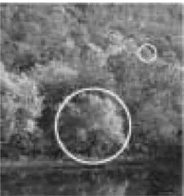
fundamen-tal concept of scale, lying everywhere in the physics world. It is easy to be convinced of the importance of this concept when we look at real-world images be-cause images are naturally composed of objects which are meaningful only at a given scale of observation. As example (Lindeberg, 1994), let us consider the forest picture on Figure 1.
At very fine scales of observation (centimeter), the leaves are the significant objects, at intermediate scales of observation (meter), the trees are the meaningful
Figure 1. Illustration of a multiscale image. At fine scales (little white circle), leaves are significant, at intermediate scales, trees are relevant (large white circle) and finally at large scales, the whole forest is significant.
objects and at the large scales of observation (kilome-ter), this is the whole forest which is significant. In other words, the way we perceive the world depends on the scale of observation we use, inspired by the scale principle of Morse, 1994. This observation has a deep impact in physics because different theories have been developed to observe the very small and the very large scales of the physics world leading to quantum mechanics and relativity theory. Even the human visual system has integrated the concept of scale in its way to capture the real-world images since psychophysical and electro-physiological studies (Hubel and Wiesel, 1979; Hubel, 1988; Zeki, 1993) have shown that the retina receives the image signal with a wide range of sampling apertures/scales (Romeny, 1997).
Since natural images are composed of structures at different scales of observation, it is then natural to de-fine a multiscale representation of an image in order to observe it at different scales. Another motivation to develop such a representation is to design methods for automatically analyzing information and deriving specific applications in computer vision. How can we design a multiscale image representation or how can we decompose an image at different scales of obser-vation/resolution? The answer of these questions are scale spaces. The main principle of scale spaces is to decrease the amount of information in images by simplifying/smoothing objects lying in them, starting from fine scales and ending to coarse scales. Mathe-matically speaking, scale spaces are hierarchical de-compositions/representations at a continuum of scales, embedding the original image I0: RN →R into a
fam-ily I : RN×[0,∞[→R of gradually more simplified versions.
The mathematical methods that generate scale spaces are generally based on partial differential equa-tions coming from diffusion processes in physics and special mathematical properties and invariances. For instance, the first scale space that has been discovered by Iijima, Witkin, Koenderink (1999, 1983, 1984) is the linear/Gaussian scale space produced by the lin-ear diffusion equation: ∂tI = I, I (t = 0) = I0,
which satisfies the conditions of linearity, causality, semi-group property, maximum principle, non-creation of local extrema at larger scales (this holds only for 1-dimensional signals), translation, rotation and scale invariances. Many other scale spaces can be defined from (non-linear) PDEs, satisfying different proper-ties, such as the scale spaces produced by the Perona-Malik model (Perona and Perona-Malik, 1990), the mean cur-vature flow (Osher and Sethian, 1988; Alvarez et al., 1993; Sapiro and Tannenbaum, 1993), the total varia-tion funcvaria-tional (Rudin et al., 1992), the Beltrami flow (Sochen et al., 1998) and others.
Finally, let us mention that the theory of scale spaces is a young theory that is constantly under development with strong mathematical bases. First applications of this theory have been to develop primitive differential operators which can change their scales of resolution to fit different unknown scales of real-world objects lying in images and thus extract specific local information from images such as edges, ridges and corners (Rudin et al., 1992; Romeny, 1994; Florack, 1993). In the fol-lowing work, we propose a multiscale image segmen-tation model to extract multiscale structures in scale spaces. Let us directly emphasize that our multiscale segmentation model has a different purpose than clas-sical multiscale models, which baclas-sically work scale by scale in order to speed up the segmentation process to-ward a global optimal solution at the inner scale, the scale of the given image. Our approach is different. We want to take into account in the segmentation process the multiscale nature of real-world images that contain objects/structures meaningful at given scales of obser-vation and which are linked through scale because fine structures are included into coarser structures in a se-mantic way such as leaves are a part of trees, which are also a part of forests, see Figure 1. Thus we will use in the segmentation process all scales at the same time, i.e. the whole scale space, which is where our technique is basically different from the standard view of multi-scale segmentations. The goal of this new approach is to introduce the concept of scale in most shape anal-ysis techniques, such as segmentation, recognition or
registration, in order to improve their robustness and their performance.
Another important motivation to design an image segmentation model at all scales simultaneously is to choose a posteriori the segmentation result at a scale which can depend on the current application and which is often unknown before the analysis process. This problem often arises with the active contour model, which will be the segmentation process used in our approach.
The active contour/snake method, defined in Kass et al., Caselles et al., Kichenassamy et al. (1987, 1997, 1996), consists of finding the planar closed curve C which minimizes the intrinsic energy func-tional FG AC(C) =
C f (I0(C(s)))ds, where ds is the Euclidean arc length element and f is an edge detecting function. The standard deviation σ of the Gaussian function Gσ in the edge detecting function f (I0) := 1+γ|∇(I10∗Gσ)|2 is the scale parameter of this
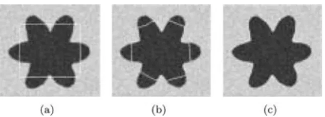
model. The active contour model needs to use an ap-propriate scale to work well. However, it is impossi-ble to know a priori which is the proper scale to get satisfactory results. The appropriate scale can depend on many parameters such as the given image, the spe-cific application, etc. Indeed, let us observe Figure 2. If the scale parameterσ is too small, the active con-tour gets stuck in noise (Figure 2(b)) and if the scale is too large, the snake approximately capture corners (Figure 2(d)). However, an appropriate scale can give satisfactory result as shown on Figure 2(c). The
prob-Figure 2. Illustration of the scale issue in the active contour model. If the scale parameter is too small, the contour gets stuck in noise, Figure 2(b) and if the scale is too large, the snake approximately captures the corners , Figure 2(d). However, there exits a correct scale for this problem that gives us a satisfactory result, Figure 2(c).
lem is that the proper scale is a priori unknown before the segmentation process. Hence, different results with different values of σ have to be tested to determine the correct scale. One solution to handle this issue is to work at different scales, which is possible with an image segmentation model working in the whole scale space, and pick up a posteriori the scale (or several scales) that looks like the most interesting for the given application.
Hence, the goal of this work is to define a multiscale image segmentation model based on the active contour model and scale spaces. We will call this new model multiscale active contours. Thus we will introduce the concept of scale in the active contour formalism (Kass et al., 1987; Caselles et al., 1997; Kichenassamy et al., 1996) to combine information from fine scales to co-arse ones in order to capture fine characteristics at low scales and extract global shape at large scales. The main question is how to mathematically design such a model, i.e. how to define an evolution equation for the active contours in scale spaces which are basically non-Euclidean/Riemannian spaces?
The answer to the previous question is given by the framework proposed by the Polyakov action that was firstly defined in high energy physics for the string the-ory (Polyakov, 1981), which basically tries to unify the four fundamental forces of nature. Then, Sochen-Kimmel-Malladi introduced this physics-based frame-work in image processing to efficiently denoise multi-dimensional images such as color and texture images (Sochen et al., 1998; Kimmel et al., 2000). The math-ematical field of the Polyakov action is the differential geometry which intrinsically describes the scale spaces such as the linear/Gaussian scale space, the Perona-Malik scale space (Perona and Perona-Malik, 1990), the mean curvature scale space (Osher and Sethian, 1988; Al-varez et al., 1993; Sapiro and Tannenbaum, 1993), the total variation scale space (Rudin et al., 1992) or the Beltrami scale space (Sochen et al., 1998), etc. Thus the geometry of scale spaces, with their intrinsic relation between space and scale/time, will be naturally intro-duced in the evolution process of the active contours in the Polyakov framework.
To summarize, the main contributions of this paper are:
(1) a general evolution equation for the active con-tours, which can be curve, surface or hypersurface, embedded in any general Riemannian manifold, (2) a multiscale image segmentation model, called
geometry of the multiscale images in the segmen-tation process,
(3) and a generalization of the gradient vector flow model to Riemannian manifolds to capture multi-scale image edges.
The next section will define a general evolution equa-tion for the active contours embedded in any general Riemannian manifold. Section 3 will present the scale spaces used in our approach. Then, we will apply in Section 4.1 the general model defined in Section 2 to embed the snake in scale spaces to define a new multi-scale segmentation process. Section 4.2 will present the model of multiscale active contours in the lin-ear/Gaussian scale space. Then, Section 5 will intro-duce the edge function we will use in our snake model to detect multiscale edges. Section 6 will generalize the gradient vector flow model to scale spaces in or-der to increase the performances of our segmentation model. Finally, we will present two multiscale results on a synthetic and a medical image in Section 7 and we will discuss our model in Section 8.
2. Weighted Polyakov Action
In (Sochen et al., 1996, 1998), Sochen-Kimmel-Malladi proposed a new general framework, based on the Polyakov action, to deal with low level processing in vision. Their new point of view considers images as surfaces embedded in higher-dimensional space. They observed that the Polyakov action is able to re-cover/generalize most of the existing scale spaces, from the linear scale space to the curvature scale space. This justifies the title of their paper (Sochen et al., 1998) since the Polyakov functional provides a single equa-tion to generalize most of scale spaces fundamental in low level vision. Moreover, they derived from this ap-proach, the Beltrami flow to efficiently denoise multi-dimensional images such as color and texture images (Kimmel et al., 2000).
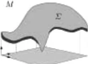
Mathematically speaking, the Polyakov action is ba-sically a functional that measures the weight of a map-ping X between an embedded manifold (e.g. the im-age manifold)and the embedding manifold M (see Figure 3). It is defined as follows: P(X, ,M)=dnςg1/2gμν∂ μXi∂νXjhi j X : (,[gμν])→(M,[hi j]) (1)
Figure 3. The manifold embedded in M, reproduced from (Sochen et al., 1998).
where [gμν] is the metric tensor/first fundamental form (Kreyszig, 1991) of the manifold, dnς is the
inte-gration element with respect to (w.r.t.) the local coordi-nates on, [hi j] is the metric tensor of the embedding space M, nis the dimension of, nMthe dimension of M, [gμν] is the inverse metric of [gμν], g is the deter-minant of [gμν],μ, ν =1, . . . ,n, i,j =1, . . . ,nM
and∂μXi =∂Xi/∂ςμ. Finally, when identical indices appear one up and one down, they are summed over according to the Einstein summation convention.
The Polyakov action, defined in (1), is related with harmonic maps which are more known as geodesics or minimal surfaces for curves and surfaces. Indeed, if the metric tensor [gμν] of the embedded manifold
is chosen to be the induced metric tensor: [gμν]=
∂μXi∂νXjhi j then the maps X which minimizes the
Polyakov action are called harmonic maps and the Polyakov functional is reduced to the Euler func-tional/Nambu action that describes the length/(hyper-) area of a curve/(hyper-)surface: S = dnς g1/2,
where g1/2is the square root of the determinant of [g
μν]
which corresponds to the infinitesimal invariant-area on
. Harmonic maps are important in geometric prob-lems because e.g. geodesics give the path of minimal distance between two points on non-flat surfaces such as a sphere. Harmonic maps are often used in image processing problems such as in image segmentation with the well-known geodesic active contour model, introduced in Section 1, which consists of finding the geodesic in a Riemannian manifold defined from the given image. This geodesic represents the boundaries of objects lying in images.
In our approach, we extend the Polyakov action in order to define a new multiscale image segmentation model. The extension is based on the introduction of a weighting function, called f , in the Polyakov functional (1) leading to the weighted Polyakov action:
Pf(X, ,M)=
dnς f (X,g
The weighted Polyakov action (2) can be minimized w.r.t. the l-th embedding coordinate Xlusing the Euler-Lagrange equations technique, gμνand hi jbeing fixed. The flow acting on Xlis then as follows:
∂Xl ∂t =g−1/2∂ μ( f g1/2gμν∂νXl)+ f ljk∂μXj∂νXkgμν −n 2 hlk∂kf g1/2gμν∂μXi∂νXjhi j, =f·g−1/2∂ μ(g1/2gμν∂νXl)+ ljk∂μXj∂νXkgμν +∂kf gμν∂μXk∂νXl−n2h lk∂kf g1/2gμν∂μXi∂ νXjhi j, for 1≤l≤nM, (3)
where g−1/2∂μ(g1/2gμν∂νXl) is the Laplace-Beltrami operator which generalizes the Laplace operator to non-flat manifolds, g−1/2∂
μ( f g1/2gμν∂νXl) is the
anisotropic Beltrami operator and l jk= 12g
li(∂ jgik+
∂kgji−∂igjk) is the Levi-Civita connection coefficients (Kreyszig, 1991).
Naturally, the metric tensor [gμν] of the embedded manifoldis chosen to be the induced metric tensor in order to work with harmonic maps and the weighted Polyakov action is then reduced to the weighted Euler functional/Nambu action that describes the weighted length/(hyper-)area of a curve/(hyper-)surface:
Sf =
dnς f g1/2. (4)
As we previously said, it is consistent to work with harmonic maps when we try to recover the model of geodesic active contours (Caselles et al., 1997). The induced metric tensor is introduced in the flow (3), which yields to:
⎧ ⎪ ⎪ ⎨ ⎪ ⎪ ⎩ ∂Xl ∂t = fH l+∂ kf gμν∂μXk∂νXl−nM2·n∂kf hkl, Hl =g−1/2∂ μ(g1/2gμν∂νXl) + l jk∂μXj∂νXkgμν gμν=∂μXi∂ νXjh i j (5) for 1 ≤ l ≤ nM andHis the mean curvature vector generalized to any embedding manifold M.
Functional (4) and its minimization flow (5) repre-sent the general equations of an active contour (curve/ surface/hypersurface) embedded in any Riemannian manifold. These general equations can be used to re-cover the classical model of geodesic/geometric active contours (Caselles et al., 1997; Kichenassamy et al., 1996) and to derive a new model for the active con-tours propagating in multiscale images. This new snake model will be developed in Section 4.1 and will be
called multiscale active contours. Let us start by recov-ering the model of geodesic/geometric active contours and its level set version.
Application 1: The geodesic/geometric active con-tours model (Caselles et al., 1997; Kichenassamy et al., 1996) evolving in a 2-D Euclidean space is recovered by choosing the following mapping and metric tensor of the embedding space M:
X :=C : q→(x(q),y(q))
hi j=δi j
(5)
Introducing (5) in (4) and (5), we obtain:
Sf =FG AC =
C f ds
∂tC=(fκ− ∇f,N)N,
which exactly corresponds to the energy and the evolution equation of the geodesic/geometric active contours model studied in Caselles et al., Kichenas-samy et al. (1997, 1996).
Application 2: The evolution equation of the level set (Osher and Sethian, 1988; Osher, 2003) version of the geodesic/geometric active contours model can also be revisited by choosing
X : (x1, . . . ,xn)→(x1, . . . ,xn, φ)
[hi j]=[δi j] (6)
Introducing (6) in (4) and (5), we obtain: ⎧ ⎪ ⎪ ⎪ ⎪ ⎪ ⎨ ⎪ ⎪ ⎪ ⎪ ⎪ ⎩ Sf = f1+ |∇φ|2 1≤i≤n d xi ∂tφ=√ 1 1+|∇φ|2∇. f√∇φ 1+|∇φ|2 =√ 1 1+|∇φ|2 fKE S+ ∇f,√∇φ 1+|∇φ|2 , (7) whereKE S = ∇. ∇φ √ 1+|∇φ|2
corresponds to the mean curvature of the surfaceembedded in an Euclidean space (ES). For 2-D surfaces, it is equal to:
KE S = (1+φ2 x)φyy−2φxφyφx y+(1+φ2y)φx x (1+φ2 x+φ2y)3/2 , (8) It is important to notice that the mean curvatureKE S is different to the mean curvatureκ = ∇ ·
∇φ
|∇φ|
of the level sets ofφ in the classical model (Osher and Sethian, 1988; Alvarez et al., 1993; Caselles et al., 1997; Kichenassamy et al., 1996). We also observe that equations (7) are not exactly the corresponding
formula of the level set version of the active contours model which are as follows:
⎧ ⎨ ⎩ F= f|∇φ| 1≤i≤n d xi ∂tφ= ∇. f |∇∇φφ| |∇φ| =fκ+ ∇f,|∇∇φφ| |∇φ|. (9) The level set flow defined in Equation (7) is equiva-lent to the following flow:
∂tφ= fKE S+g−E S1/2∇f,∇φ |∇φ|, (10) = fKE S+ g−E S1/2|∇φ| =:r (φ) ∇f, ∇φ |∇φ| |∇φ|, (11) since the solution of an Euler-Lagrange equation is not changed when the Euler-Lagrange equation is multi-plied by a strictly positive function such as g1E S/2·|∇φ| = (1+ |∇φ|)1/2· |∇φ|. According to the general formula
∂tφ = F|∇φ| ⇒ ∂tC = FN, Equation (11) implies that the level sets ofφmove according to the equation:
∂tC=(fKE S−r (φ)∇f,N) N, (12) where N = −∇φ/|∇φ| is the unit normal to the level sets. Thus, Equation (12) is close to the evolu-tion equaevolu-tion of the geodesic/geometric active contours
∂tC=(fκ− ∇f,N)Nup to the surface mean cur-vatureKE Sand the function r . However both evolution equations have the same behavior, i.e. smoothing and attraction toward edges. Function r can be interpreted as an indicator of the height variation on the surface
(see Aubert and Kornprobst, 2001). Indeed, g−E S1/2 is the ratio between the area of an infinitesimal sur-face in the domain (x,y) and the corresponding area on the surface. For flat surfaces, r is goes to 0 and it is close 1 near edges. Finally, the function r is con-stant almost everywhere when φis a signed distance function.
Equations (4) and (5) allowed us to recover the model of active contours/snakes in the explicit and the implicit representations. Both representations, the contour C and the level set functionφ, were embedded/evolved in Euclidean spaces defined by the Euclidean metric tensor [hi j] = [δi j]. However, Equations (4) and (5) were established for general embedding Riemannian manifolds. Hence, it is possible to change the embed-ding space for the active contours and consider the scale spaces. The natural next question is which scale spaces
can be used in our framework? The question was an-swered by Eberly in 1994a who defined a family of scale spaces that includes the linear scale space, the Perona-Malik scale space, the curvature scale space and the Beltrami scale space.
3. Scale Spaces
In (Eberly, 1994a, 1994b) Eberly studied the geometry of a large class of scale spaces and defined for them the general metric tensor:
hi j = diag 1 c2In, 1 c2ρ2 , (13) where n is the spatial dimension,Inis the n×n identity matrix, c andρ are two functions that physically cor-respond to the conductance and the density functions in the general model of heat diffusion transfer. These functions can depend on space, scale and image data. As Eberly said in (Eberly, 1994), the natural diffusion equation in any space defined by a metric tensor is obtained as follows: the left-hand side of the diffusion equation is given by one application of the scale deriva-tive and the right-hand side by two applications of the spatial derivative. In the case of scale spaces, defined by the metric tensor (13), the scale derivative and the spa-tial derivative are given by the scale space (SS) gradient defined by the covariant derivative (Kreyszig, 1991):
∇SS :=[hi j]−T∇x,σ = ⎛ ⎜ ⎝c∂x1, . . . , c∂xn spatial derivative , ρ c∂σ scale derivative ⎞ ⎟ ⎠=(c∇, ρc∂σ) (14) where [hi j] is the inverse tensor of [h
i j], T means the transpose operator, [hi j]−T := ([hi j]−1)T and ∇x,σ :=(∂x
1, . . . , ∂xn, ∂σ) =(∇, ∂σ) where∇ stands
for the Euclidean space gradient. Hence, the natural diffusion equation is defined by
(ρc∂σ) I =(c∇)·(c∇) I, (15)
∂σI = 1ρ∇ ·(c∇I ). (16)
Equation (16) is the general model of heat diffusion transfer that generates different multiscale image
representations, i.e. scale spaces, by applying a PDE which is a non-linear anisotropic diffusion equation in its general expression.
Different choices of the functions c andρgive dif-ferent scale spaces with difdif-ferent diffusion equations (16), which emphasizes well the close relation between multiscale image analysis/scale space and diffusion processes that originate from physics. For example, the most popular scale space can be recovered when c=σ (the scale parameter) andρ = 1:∂σI =σI . Other well-known scale space can be derived from the metric tensor (13) and the associated multiscale generation process (16). For example, the Perona-Malik scale space (Perona and Malik, 1990) is obtained whenρ=1 and c = exp(−α|∇I|2), α > 0: ∂σI = ∇ ·(c∇I ). The famous mean curvature flow, which is one of the fundamental equation in image processing (Osher and Sethian, 1988; Alvarez et al., 1993; Sapiro and Tan-nenbaum, 1993), is obtained by setting c =ρ= |∇1I|:
∂σI = ∇.(|∇∇II|)|∇I| = κ|∇I , where κ is the mean curvature of the level sets of I . We can also use the Bel-trami flow of Sochen-Kimmel-Malladi (Sochen et al., 1996, 1998) with c = ρ = √ 1
1+|∇I|2: ∂σI = gI ,
wheregis the Laplace-Beltrami operator.
4. Multiscale Active Contours
4.1. The General Case
In this section, we define the general evolution equation for the active contours in the scale spaces defined in the previous section. We use the results obtained in Section 2, the weighted Polyakov action, to determine the evolution equation of the active contours and the associated energy in scale spaces. The harmonic map X , the metric tensor [hi j] of the embedding scale space and the metric tensor [gμν] of the level set surfaceφ manifold representing the active contour are chosen as follows: ⎧ ⎪ ⎪ ⎪ ⎨ ⎪ ⎪ ⎪ ⎩ X : (x1, . . . ,xn, σ)→(x1, . . . ,xn, σ, φ) [hi j]= diag 1 c2In,c21ρ2,c12 =:hSS i j [gμν]=∂μXi∂ νXjhi j=: gSS μν (17)
where x1, . . . ,xnare the n spatial components andσis the scale parameter. Then, the previous Equations (17) are introduced in Functional (4) and its minimization
flow (5) leading to: Sf = dnσ f g1/2 ∂tXl=fHl+∂kf gμν∂μXk∂νXl−nM2·n∂kf h kl (18)
which leads to the energy functional and the evolution equation for the (n+2)-th component of X , i.e. the level set componentφ, which embeds the multiscale active contour (MAC):
⎧ ⎪ ⎨ ⎪ ⎩ EM AC = f1+ |∇φ|2+ρ2φ2 σ 1≤i≤n d xi c dσ cρ ∂tφ =g−SS1/2fKSS+ ∇x,σ f,∇x,σφ[gμνSS] (19) where f = f (x1, . . . ,xn, σ), gSS = c2(n+11)ρ2(1 + |∇φ|2 +ρ2φ2 σ) is the determinant of [gμνSS],d xci dσ cρ
corresponds to the infinitesimal invariant volume in the scale spaces defined by the metric tensor (13), ∇x,σ :=(∇, ∂σ),.,.
[gμνSS]is the inner product in
mani-folds (,[gμνSS]) such that V1,V2[gμνSS]:=V
T
1
gμνSSV2=V1μgμνSSV2ν, (20)
andKSS is the (n+2)-th component of the mean cur-vature vector (5) (up to g−1/2) generalized to scale
spaces: KSS = ∂μ(g1/2gμν∂νXl) (21) +g1/2 l jk∂μX j∂ νXkgμνgSS μν=∂μXi∂νXjhi jSS.
By analogy with Section 2, we look for the evolution equation of the level sets of φ which zero level set represents the multiscale active contour. The evolution equation of the level set functionφdefined in Equation (19) is equivalent to the following flow:
∂tφ= fKSS+g1SS/2∇x,σf,∇x,σφ[gμνSS] |∇x,σφ|, (22) =fKSS+g1SS/2|∇x,σφ| =:rSS(φ) ∇x,σφ, ∇x,σφ |∇x,σφ| [gμνSS] , (23) since the solution of an Euler-Lagrange equation is not changed when the Euler-Lagrange equation is multi-plied by a strictly positive function such as g1SS/2 · |∇x,σφ|. According to the general formula ∂
tφ= F|∇φ| ⇒ ∂tC = FN, Equation (23) implies that the level sets ofφmove according to the equation:
∂tC =
fKSS−rSS(φ)∇x,σf,N
whereN = −∇x,σφ/|∇x,σφ|is the unit normal to the
level sets.
In the rest of this section, we develop some equa-tions for n = 2, i.e. 2-D images, that will be used to experiment with our multiscale segmentation model. The harmonic map X and the metric tensor [hi jSS] of embedding scale spaces for n =2 have the following form: X : (x,y, σ)→(x,y, σ, φ) hSS i j = diag 1 c2,c12,c21ρ2,c12 (25)
Then, the metric tensor [gSS
μν], its determinant gSS and its inverse metric [gμνSS] are as follows:
⎧ ⎪ ⎪ ⎪ ⎪ ⎪ ⎪ ⎪ ⎪ ⎪ ⎪ ⎪ ⎪ ⎨ ⎪ ⎪ ⎪ ⎪ ⎪ ⎪ ⎪ ⎪ ⎪ ⎪ ⎪ ⎪ ⎩ gSS μν = 1 c2 ⎛ ⎝1+φ 2 x φxφy φxφσ φxφy 1+φ2 y φyφσ φxφσ φyφσ ρ12+φσ2 ⎞ ⎠ gSS = 1 c6ρ2 1+φ2 x+φ2y+ρ2φσ2 gSSμν= 1 gc41ρ2· ⎛ ⎜ ⎝ 1+φ2 y+ρ2φσ2−φxφy −ρ2φxφσ −φxφy 1+φ2 x+ρ2φσ2−ρ2φyφσ −ρ2φxφ σ −ρ2φyφσ ρ2 1+φ2 x+φ2y ⎞ ⎟ ⎠ (26)
The energy functional of the multiscale active contours for n=2 is EM ACSS = f ! 1+φ2 x+φ2y+ρ2φσ2 d xd ydσ c3ρ (27)
The general evolution equation of multiscale active contours for n = 2 is very long! Hence, it is easier to develop the evolution equation of active contours in specific scale spaces. In this work, we choose to use the most well-known scale space, i.e. the linear scale space. Obviously, other scale spaces can be used in our segmentation framework. In the future, it will be in-teresting to develop the curvature scale space which efficiently preserve multiscale edges to carry out the segmentation and the shape recognition tasks on real-world applications.
4.2. Active Contours in the Linear Scale Space The first natural application of the previous multiscale segmentation model is in the linear scale space, ob-tained when the conductance function is equal to c=σ (the scale parameter) and the density function is equal toρ =1. We consider the case n =2 of 2-D images.
In this situation, the energy of the multiscale active contour and the flow applied on the level set function
φ (embedding the active contour) in the linear scale space are equal to:
EM ACL SS = f ! 1+φ2 x+φ2y+φ2σ d xd ydσ3 σ, ∂tφ =g−L SS1/2fKL SS+gL SS−1 σ12∇x,σf,∇x,σφL SS, (28) where gL SS = σ16(1+φ2x +φ2y +φσ2) andKL SS is the mean curvature in the linear scale space computed using Equation (22): KL SS=g−L SS1/2 φμν σ6 g μν L SS (1) −3g1L SS/2 φμ σ gμσ (2) . (29)
The first part of the mean curvature (29.1) in the linear scale space corresponds to the Euclidean part because the Euclidean mean curvature is equal to g−E S1/2φμνgμνE S whenσ =1, and the second term (29.2) corresponds to the Riemannian part. More explicitly, Equation (29) is equal to: KL SS=σ1 1+φ2 x+φ2y+φ2σ −3/2 · φx x 1+φ2 y+φ2σ +φyy 1+φ2 x+φσ2 +φσσ1+φ2x+φ2y −2φx yφxφy−2φxσφxφσ −2φyσφyφσ−3σ12 1+φx2+φ2y+φσ2−3/2·φσ (30)
Finally, ·,·L SS in Equation (28) is the inner prod-uct in the linear scale space defined byV1,V2L SS=
1 σ2V1,V2such that: 1 σ2 1 gL SS∇ x,σf,∇x,σφL SS = σ2 1+φ2 x+φ2y+φσ2( fxφx+ fyφy+ fσφσ). (31)
5. Multiscale Image Features
The previous sections introduced the segmentation model of multiscale active contours which is able to extract multiscale objects in multiscale images. The extraction process is based on a PDE (19) defining an evolution equation for hyper-surfaces in non-Euclidean manifolds, the scale spaces, which capture multiscale image features represented by the function f in the flow∂tφ=g−SS1/2fKSS+ ∇x,σf,∇x,σφ[gμνSS]. Which
are the possible functions f to capture local multiscale edges?
5.1. Classical Multiscale Edge Detecting Function By analogy with the classical model of geomet-ric/geodesic active contours (Kass et al., 1987; Caselles et al., 1997; Kichenassamy et al., 1996), the most com-mon multiscale edge detecting function to capture mul-tiscale structures is based on the norm of the image gradient:
f = 1
1+β|∇SSI (x1, . . . ,xn, σ)|2, (32)
whereβ is an arbitrary positive parameter,∇SS is the scale space gradient defined in Equation (14) such as |∇SSI| = (c2I2 x1+ · · · +c 2I2 xn+c 2ρ2I2 σ)1/2 and I is
a multiscale image obtained by applying a PDE such as Equation (16) on a given image I0. The definition
of the edge detecting function (32) is easy to establish without technical particularities. However, it is possi-ble to define an enhanced multiscale edge detecting function with the work of Eberly (1994a) who studied many image features in a strong mathematical frame-work based on differential geometry. In our approach, we will consider special image features called ridges.
5.2. Multiscale Edge Detecting Function Based on Ridges
In (Eberly, 1994a), Eberly explored various ways to detect local image features, called ridges, in n-dimensional spaces. Ridges play an important role in the characterization of semantic local features. Gener-ally speaking, ridges are image features of a function which have local maximum in f along the direction of the greatest concavity (Morse, 1994). Thus, at a ridge point the direction of greatest curvature is the cross-ridge direction and the value of the function is greater than the neighboring points on either side of it. Figure 4 illustrates a line of ridge points.
Figure 4. Ridges as maxima in the direction of the greatest curva-ture, reproduced from (Morse, 1994).
Ridges can be defined by different ways (Eberly, 1994a). In our approach, we use the definition devel-oped in Section 2.3 of (Eberly, 1994a). A point in an n-D space is an m-D ridge (m<n) of a functionFif:
λi <0
ei,∇F =0 for all i<n−m, (33) where (λ1, . . . , λn) with |λ1| ≤ · · · ≤ |λn| and (e1, . . . ,en) are the eigenvalues and the corresponding eigenvectors of the Hessian ofF, which is the n×n matrix of the second derivatives ofF. The Hessian is a fundamental quantity in geometry because it is related with the intrinsic geometry of the n-graph indepen-dently of the surface parametrization. It is important to notice that the Hessian computed in an Euclidean space is different in a Riemannian space. The scale space Hessian∇2
SSis obtained according to the follow-ing equation (Kreyszig, 1991; Eberly, 1994):
∇2 SS := "# hi jSS $−Tdc∇x,σf dcξSS "# hi jSS $−1 , (34) whereξSS =(x1, . . . ,xn, σ) anddc∇ x,σf dcξSS is the
covari-ant derivative of∇x,σf , which is a second-order tensor defined by: dc∇x,σf dcξSS = % ∇x,σ2f − n+1 & k=1 k (∇x,σf )k ' , (35) where ∇x,σ2 stands for the Euclidean Hessian,
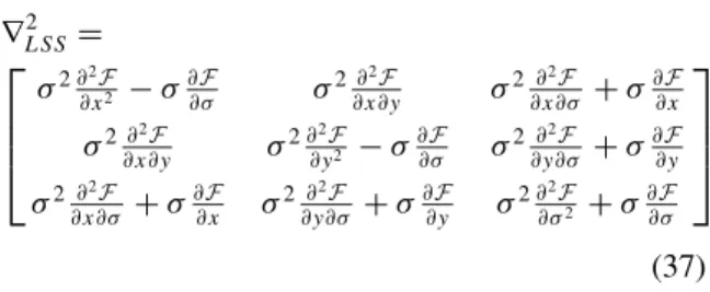
(∇x,σf )k is the k-th component of ∇x,σ f and k is the k-th Levi-Civita connection coefficient of [hi jSS]. In the practical case of 2-D images, i.e. when n = 2, and considering the linear scale space with c=σ and
ρ =1, then the Hessian, which takes into account the particular interdependence between space and scale, is equal to (Morse, 1994): ∇2 L SS= ⎡ ⎢ ⎢ ⎣ σ2∂2F ∂x2 −σ∂∂σF σ2∂ 2F ∂x∂y σ2∂ 2F ∂x∂σ +σ∂∂Fx σ2∂2F ∂x∂y σ 2∂2F ∂y2 −σ∂∂σF σ2∂ 2F ∂y∂σ +σ∂∂Fy σ2 ∂2F ∂x∂σ +σ∂∂Fx σ 2∂2F ∂y∂σ +σ∂∂Fy σ 2∂2F ∂σ2 +σ∂∂σF ⎤ ⎥ ⎥ ⎦ (37) Equations (33) and (36) allow us to compute mul-tiscale ridges for a function F to be chosen. In our approach, we decide to extract ridges from the norm of the scale space gradient of the multiscale image I ,
i.e.F = |∇L SSI (x,y, σ)| =σ·(I2
x+Iy2+Iσ2)1/2,
us-ing Equation (33). The result of this process is a binary function, namely 1ridges(x,y, σ) which is equal to 1 for ridge points and 0 otherwise. Then, the function 1ridges is multiplied by the multiscale norm|∇L SSI|to weight the ridge points. Finally, our edge detecting function is given by the equation:
f = 1
1+β(1ridges· |∇L SSI|),
(36) which means that f is equal to 1 on homogeneous regions as in the classical model of geometric/geodesic active contour (Kass et al., 1987; Caselles et al., 1997; Kichenassamy et al., 1996).
6. Multiscale Gradient Vector Flow
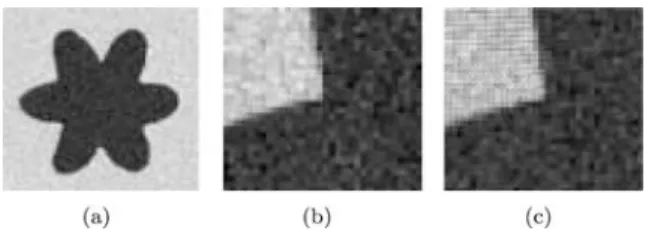
Section 4 proposed a multiscale segmentation flow (19) which is able to capture structures, represented by (32) and (36), in scale spaces defined in Section 3. The seg-mentation process is completely defined however it is very slow as the process of geometric/geodesic active contours. This is due to the edge detecting function f and its gradient∇x,σf in (19) which are only “active” close to object edges. Indeed, when the active contour is far from edges, the gradient of f is close to zero and f is nearly equal to 1, which means that only the cur-vature acts, which is a slow evolution process. When the active contour is close to edges, then the gradi-ent of f becomes active and attract the snake toward the edges. The evolution process could be speed up if the active contour was attracted by the edges in homo-geneous/smooth regions. This issue was solved by Xu-Prince in (Xu and Xu-Prince, 1998) who proposed a method called the gradient vector flow (GVF) which can extend the multiscale gradient field of f into smooth regions and also deal with the problem of concave regions. In the following, we firstly present the original model of Xu-Prince which is designed to work in Euclidean spaces. Then, we will extend the model to scale spaces. 6.1. Gradient Vector Flow in Euclidean Spaces The gradient vector flow model was originally devel-oped to overcome the issues of contour initialization and poor convergence to boundary concavities in the geometric/geodesic active contours model (Kass et al., 1987; Caselles et al., 1997; Kichenassamy et al., 1996). For example, Figure 5 presents an object with concave
Figure 5. Figure (a) presents an object which boundary is a har-monic curve. Figure (b) shows the gradient of the given image and Figure (c) presents the extended image gradient using the GVF method.
concavities which can not be fully segmented with clas-sical geometric/geodesic active contours (even with a balloon force (Cohen, 1991)) since the snake can not go inside concave parts of the given object. Moreover, the convergence of the classical active contours model is slow compared with the method proposed by Xu-Prince in (Xu and Prince, 1998) even if the initial contour is satisfactory. Xu-Prince propose to diffuse/extend the image gradients into smooth regions while preserving edge forces. Their method is defined in a variational framework since the GVF field minimizes the follow-ing energy functional in the n-D Euclidean space:
FGV F E S (V)= μ . n & i=1 |∇Vi|2 / (1) + |∇ f|2|(V− ∇f )2 (2) dx, (37)
where f (x1, . . . ,xn) is the initial data n-D function,
V(x1, . . . ,xn) = (V1, . . . ,Vn) is the gradient vec-tor field minimizing Functional (37) and extending the original gradient of f in homogeneous/smooth re-gions, μ is an arbitrary constant which balances the contributions between the diffusion and regularization term (37.1) and the data fidelity term (37.2). Indeed, if
μ→0 then the solution is V= ∇f and ifμ→ ∞then
V is solution of the classic isotropic diffusion
equa-tion 0ni=1|∇Vi|2. Moreover, when the norm of gra-dient|∇f|is small in (37), i.e. in smooth regions, the term (37.2) is also small and Energy (37) minimizes the diffusion-based term (37.1) by propagating the vector field V. Inversely, when the norm of gradient|∇f|is large, i.e. on edges, the second term (37.2) dominates and constraints the vector field V to be equal to the original data∇f .
The minimization of Energy functional (37) is done using the calculus of variations and the gradient descent method which provide n flows, one per component of
Figure 6. Figure (a) presents the initial active contour. Figure (b) is the final contour using the classic image gradient on Figure 5(b) and Figure (c) is the final contour using the GVF method on Figure 5(c).
the GVF field. The Frechet derivative of FE SGV F w.r.t. Vi in theξ-direction is ∂FGV F E S ∂Vi , ξ = (38) ξ· % −μ . n & j=1 ∂2 xjVi / + |∇f|2(Vi−∂xi f ) ' dx, for 1≤ i ≤n. Then, the flow minimizing FGV F
E S w.r.t. Vi is ∂Vi ∂t =μ . n & j=1 ∂2 xjVi / − |∇f|2(V i−∂xif ), (39) for 1≤ i ≤n.
Let us apply the GVF model to Figure (5.a). Fig-ure (5.b) presents the image gradient and FigFig-ure (5.c) the extended image gradient computed with Equations (39). Finally, Figure 6 illustrates the usefulness of the GVF method since the geodesic/geometric active con-tours model which uses the classic image gradient can not fully segment the harmonic boundary whereas the gradient vector flow allows us to completely segmented the boundary.
6.2. Gradient Vector Flow in Scale Spaces
The previous section introduced the GVF method which basically extends the image gradient in homoge-neous/smooth regions to faster capture image edges and to deal with concave and convex object boundaries. The previous method was defined in n-D Euclidean spaces but we will generalize it into scale spaces by taking ac-count the special relation between space and scale using the metric tensor (13). We will use the multiscale gra-dient vector flow model to extend the multiscale edge detecting function (32) or (36) into smooth regions to efficiently capture multiscale objects in multiscale im-ages.
The Euclidean GVF model is extended to scale spaces by simply “updating” the Euclidean quantities to their Riemannian equivalents. Thus, the Euclidean gradient∇is replaced by the scale space gradient∇SS and the Euclidean infinitesimal invariant volume ele-ment dx by the scale space one dxSS, Energy functional (37) then becomes: FSSGV F(V)= μ . n & i=1 |∇SSVi|2 / (40) + |∇SSf|2(V− ∇SSf )2dxSS,
Considering the scale space gradient∇SS=(c∇, ρc∂σ)
and dxSS =
1≤i≤n d xi
c dσ
cρ, the Frechet derivative of FGV F
SS w.r.t. Viin theξ-direction is: 1 ∂FGV F SS ∂Vi , ξ 2 = ξ · % −μ . n & j=1 ∂xj(c 2∂ xjVi)+∂σ(c 2ρ2∂ σVi) / + |∇SSf|2(Vi−(∇SSf )i) ' 1 cn+1ρ dx, (41)
for 1≤ i ≤ n+1. Then, the flow minimizing FSSGV F w.r.t. Vi is ∂Vi ∂t = μ . n 0 j=1 ∂xj ∂x jVi cn−1ρ +∂σ ρ∂σVi cn−1 / −|∇SSf|2 cn+1ρ (Vi−(∇SSf )i), (42)
for 1≤ i ≤n+1. For our application, we consider the linear scale space, i.e. c=σ, ρ =1 and 2-D images, i.e. n=2: ∂Vi ∂t (x,y, σ)= μ(σ −1∇x,σ2 Vi−σ−2∂σVi) −σ−1|∇x,σf|2(V i−σ∂if ), for i=x,y, σ, (43) where∇x,σ2= ∇2+∂2 σand∇x,σ =(∇, ∂σ). 7. Results
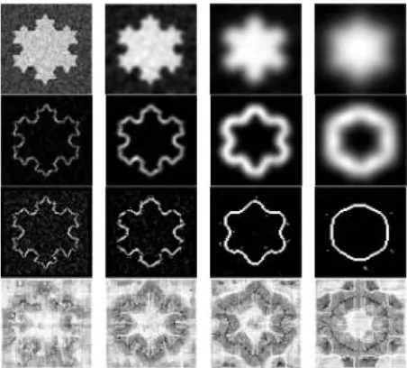
In this section, we apply our multiscale image segmen-tation model in the linear scale spaces of two images: a 64×64 synthetic image based on the Von Koch’s picture, corrupted with additive Gaussian noise and a
Figure 7. First row presents the linear scale space of the Von Koch’s picture at four different scales of observation. Second row shows the norm of the linear scale space gradient and third row presents the ridges of the scale space image gradient norm. Fourth row gives the multiscale GVF.
64×64 brain magnetic resonance image. The number of scales for both pictures is 15.
The first row of Figures 7 and 8 present the linear scale space of the Von Koch’s picture and the brain picture at four different scales of observation. The sec-ond row of Figures 7 and 8 show the norm of the linear scale space gradient. The third row present the multiscale edge detecting function, defined in Equa-tion (36), based on the ridge points detected from the norm of the linear scale space gradient. The multi-scale ridges, defined in Equation (33), are robustly extracted with the approach of Morse, Chapter 7 in Morse (1994). The fourth row of Figures 7 and 8 show the multiscale GVF. The initial vector field is chosen to be the scale space gradient of the edge de-tecting function (36), i.e. V(t = 0) = ∇L SSf . The multiscale GVF, Equation (43), is implemented using central approximation schemes for spatial derivatives and the scale derivative scheme proposed by Eberly (1994, 1994a). The run times are about 5 minutes for the Von Koch’s picture and 15 minutes for the brain picture.
The segmentation process is given by the flow (28). It is implemeted as follows: the mean curvature
KL SS, developed in Equation (30), is implemented, like GVF, using central approximation schemes for spa-tial derivatives and the scale derivative scheme pro-posed by Eberly (1994, 1994a). The advection term, Equation (31), is discritized with standard upwind schemes based on hyperbolic conservation laws, see e.g. Osher (2003) or Sethian (1999). Furthermore, the level set function is periodically re-initialized with the fast marching method of Adalsteinsson-Sethian (1995).
First row of Figures 9 and 10 present the evolution of the active contour, which is a surface in this case, in the linear scale space and the last three rows show the evolution process of the multiscale snake at four differ-ent scales. The run times of the segmdiffer-entation process are about 5 minutes for the Von Koch’s picture and 15 minutes for the brain picture.
8. Conclusion, Comparison and Future Research
In this paper, we defined a method to extract objects lying in images at different scales of observation. As we explained in Section 1, the multiscale nature of
Figure 8. First row presents the linear scale space of a 2-D brain image at four different scales of observation. Second row shows the norm of the linear scale space gradient and third row presents the ridges of the scale space image gradient norm. Fourth row gives the multiscale GVF.
images, discovered by Iijima, Witkin, Koenderink (Weickert et al., 1999; Witkin, 1983; Koenderink, 1984), makes this image segmentation method relevant because real-world images contain objects meaningful
Figure 9. First top row presents the multiscale active contour evolv-ing in the linear scale space and the last four row show the active contour propagating at four different scales.
at given scales of observation and which are linked through the scale because fine structures are included into coarser structures in a semantic way.
Moreover, the multiscale paradigm used in this paper implies that all solutions to a given image analysis prob-lem, corresponding to different scales of observation,
Figure 10. First top row presents the multiscale active contour evolving in the linear scale space and the last four row show the active contour propagating at four different scales.
are valid! The choice of a “correct” scale is significant only for a given application, which “fixes” the scale, but all solutions are relevant. That is why we considered all scales in our approach, i.e. all possible solutions, to the segmentation problem.
Unlike classical multiscale segmentation models, that have already been proposed by e.g. Leroy-Herlin-Cohen in (Leroy et al., 1996), we do not use the multi-scale concept to speed up the convergence toward the global optimal solution. Indeed, the authors in (Leroy et al., 1996) proposed to use the Gaussian scale space to speed up the convergence of the active contour model as follows: first, the snake solution is determined at a coarse scale, then the final contour is used as initial-ization at a finer scale. This process is iterated until the finest scale. This multiscale segmentation process allow first to avoid bad local minima, corresponding to bad segmentation results, and thus obtain a local minimum close to the global optimal segmentation so-lution and second, to avoid a high computational cost to find the global solution because they work from low dimensional images, in coarse scales, to high dimen-sional one, in fine scales, still using simple optimiza-tion technique based on the gradient descent. Thus, classical multiscale segmentation models speed up the segmentation process and are robust with respect to initial condition and noise. However the main issue in this model is the fact that authors did not consider the fundamental relation between space and scale/time. In other words, they did not introduce the intrinsic geom-etry of the Gaussian scale space in the segmentation process. In our work, we have taken into account the geometry of the Gaussian scale space, and other scale spaces, in the segmentation process. Our multiscale im-age segmentation model used the important geometric information of scale spaces, which was not the case in the previous works. Thus we performed the segmenta-tion process at all scales simultaneously and we also found a solution close to the optimal global solution. Indeed, like classical multiscale segmentation models, our model can avoid bad local minima at finer scales thanks to coarser scales. It is due to scale spaces, which create a basin catching in the minimization algorithm, and the mean curvature force which acts on the sur-face through scales to influence finer scales thanks to coarser scales.
Close to our approach, Schnabel-Arridge (1999) also proposed a model to extract scale by scale the shape of objects. They used the segmentation result at each scale to build a multiscale representation of the segmented
object. The extracted multiscale shapes are used to lo-calize and characterize shape changes at different levels of scale. They applied their model to segment 3-D brain magnetic resonance images in order to quantify the structural deformations for patients having epilepsy. Thus their approach is close to ours but the main weak-ness of their model is not to use the relation between space and scale/time, coded in the geometry of scale spaces.
From a mathematical point of view, the Polyakov framework, introduced by Sochen-Kimmel-Malladi (Sochen et al., 1998) in image processing, provided us the mathematical framework to use and incorpo-rate the multiscale information lying in scale spaces in the active contour segmentation process. Indeed, the Polyakov functional gave us the general evolution equation for the active contours in any Riemannian manifold defined from a first fundamental form/metric tensor. Since scale spaces, such as the Gaussian scale space, the curvature scale space or the Beltrami scale space, are natural Riemannian manifolds which metric tensors were defined from the general heat diffusion equation in Section 3. We also chose to work, like in classical approaches (Kass et al., 1987; Caselles et al., 1997; Kichenassamy et al., 1996), with harmonic maps by choosing the metric tensor of the embedded man-ifold as the induced metric tensor. The result is the model of multiscale active contours, which is able to extract multiscale structures lying in images.
Future works will be focused on integrating this multiscale segmentation technique into shape analysis methods such as the shape recognition task or the shape registration method to improve their robustness and their performance. More precisely, combining a multi-scale shape prior such as the multimulti-scale medial axis called cores and developed by Pizer-Eberly-Morse-Fritsch (Pizer et al., 1998), with our mutiscale seg-mentation model could provide an efficient multiscale recognition method. Moreover, our multiscale image segmentation model provides a multiscale shape rep-resentation that can be useful to register complex geo-metric shapes such as the brain cortical surface. Special metrics defined in multiscale spaces can be used to ef-ficiently compare shapes at different scales.
Another future work will be to change the linear scale space (Bresson et al., 2005), which does not preserve well the edges, into a more useful scale space such as the curvature scale space which is one of the funda-mental model in image processing (Osher and Sethian, 1988; Alvarez et al., 1993).
References
Adalsteinsson, D. and Sethian, J. 1995. “A Fast Level Set Method for Propagating Interfaces,” Journal of Computational Physics, 118, 269–277.
Alvarez, L. Guichard, F. Lions, P.L. and Morel, J.M. 1993. “Axioms and Fundamental Equations of Image Processing,” Archives For Rational Mechanics, 123(3), 199–257.
Aubert, G. and Kornprobst, P. 2001. Mathematical Problems in Im-age Processing: Partial Differential Equations and the Calculus of Variations, Springer, 147.
Bresson, X. Vandergheynst, P. and Thiran, J.-P. 2005. “Multiscale Active Contours,” in Proceedings of 5th International Conference on Scale Space and PDE methods in Computer Vision, 167–178, Caselles, V. Kimmel, R. and Sapiro, G. 1997. “Geodesic Active Con-tours,” International Journal of Computer Vision, 22(1), 61–79. Cohen, L.D. 1991. “On Active Contour Models and Balloons,”
Com-puter Vision Graphics Image Processing, 53, 211–218. Eberly, D. 1994. “A Differential Geometric Approach to Anisotropic
Diffusion in Geometry-Driven Diffusion in Computer Vision,” Computational Imaging and Vision, 1, 371–392.
Eberly, D. 1994. “Geometric Methods For Analysis Of Ridges In n-Dimensional Images, Ph.D Thesis, University of North Carolina.” Kreyszig, E. 1991. Differential Geometry, Paperback.
Florack, L. 1993. “The Syntactical Structure of Scalar Images, Ph.D Thesis, University of Utrecht.”
Hubel, D.H. and Wiesel, T.N. 1979. “Brain Mechanisms of Vision,” Scientific American Press, 241, 45–53.
Hubel, D.H. 1988. “Eye, Brain and Vision,” Scientific American Press, New York.
Kass, M. Witkin, A. and Terzopoulos, D. 1987. “Snakes: Active Contour Models,” International Journal of Computer Vision, 321– 331.
Kichenassamy, S. Kumar, A. Olver, P. Tannenbaum, A. and Yezzi, A.J. 1996. “Conformal Curvature Flows: From Phase Transitions to Active Vision,” in Archive for Rational Mechanics and Analysis, 275–301, 134.
Kimmel, R. Malladi, R. Sochen, N. 2000. “Images as Embedded Maps and Minimal Surfaces: Movies, Color, Texture, and Volu-metric Medical Images,” International Journal of Computer Vi-sion, 39(2), 111–129.
Koenderink, J.J. 1984. “The Structure of Images,” Biological Cyber-netics, 50, 363–370.
Leroy, B. Herlin, I. and Cohen, L.D. 1996. “Multi-Resolution Algo-rithms for Active Contour Models,” in Proceedings of the Twelfth International Conference on Analysis and Optimization of Sys-tems, 58–65.
Lindeberg, T. 1994. Scale-Space Theory in Computer Vision, Kluwer Academic Publishers, Netherlands.
Morse, B. 1994. “Computation of Object Cores From Grey-Level Images, Ph.D Thesis, University of North Carolina.”
Osher, S. and Sethian, J.A. 1988. “Fronts Propagating with Curvature-Dependent Speed: Algorithms Based on Hamilton-Jacobi Formulations,” Journal of Computational Physics, 79(1), 12–49.
Osher, S. 2003. “Level Set Methods”, in Geometric Level Set Meth-ods in Imaging, Vision and Graphics, eds. S. Osher and N. Para-gios, Springer-Verlag, NY, 3–20.
Perona, P. and Malik, J. 1990. “Scale-Space and Edge Detection Us-ing Anisotropic Diffusion,” IEEE Transactions on Pattern Analy-sis and Machine Intelligence, 1252, 629–639.
Pizer, S.M. Eberly, D. Morse, B.S. and Fritsch, D.S. 1998. “Zoom-Invariant Vision of Figural Shape: The Mathematics of Cores,” International Journal of Computer Vision and Image Understand-ing, 69, 55–71.
Polyakov, A.M. 1981. “Quantum Geometry of Bosonic Strings,” Physics Letters B, 103, 207–210.
Rudin, L.I. Osher, S. and Fatemi, E. 1992. “Nonlinear Total Variation Based Noise Removal Algorithms,” Physica D, 60(1–4), 259– 268.
Sapiro, G. and Tannenbaum, A. 1993. “Affine Invariant Scale-Space,” International Journal of Computer Vision, 11(1), 25–44. Schnabel, J.A. and Arridge, S.R. 1999. “Active Shape Focusing,”
Image and Vision Computing, 17(5–6), 419–428.
Sethian, J.A. 1999. Level Set Methods and Fast Marching Methods: Evolving Interfaces in Computational Geometry, Fluid Mechan-ics, Computer Vision and Material Sciences, Cambridge Univer-sity Press.
Sochen, N. Kimmel, R. and Malladi, R. 1996. “A General Framework For Low Level Vision, Technical Report LBNL-39243,” Physics Department, Berkeley.
Sochen, N. Kimmel R. and Malladi, R. 1998. “A General Framework For Low Level Vision,” IEEE Transactions on Image Processing, 7(3), 310–318.
ter Haar Romeny, B.M. (Editor), 1994. Geometry Driven Diffusion in Computer Vision, Kluwer Academic Publishers, Netherlands. ter Haar Romeny, B.M. 1997. Front-End Vision and Multiscale Image
Analysis: Introduction to Scale-Space Theory, Kluwer Academic Publishers, Netherlands.
Weickert, J. Ishikawa, S. and Imiya, A. 1999. “Linear Scale-Space has First been Proposed in Japan,” Journal of Mathematical Imag-ing and Vision, 10, 237–252.
Witkin, A.P. 1983. “Scale-Space Filtering,” in International Joint Conference Artificial Intelligence, 1019–1022.
Xu, C. and Prince, J. 1998. “Snakes, Shapes and Gradient Vector Flow,” IEEE Transaction on Image Processing, 7, 359–369. Zeki, S. 1993. A Vision of the Brain, Blackwell Scientific