Fair scores for ensemble forecasts
C. A. T. Ferro
College of Engineering, Mathematics and Physical Sciences, University of Exeter, UK ∗
Correspondence to: C. A. T. Ferro, College of Engineering, Mathematics and Physical Sciences, University of Exeter, Harrison Building, North Park Road, Exeter EX4 4QF, UK. E-mail: [email protected]
The notion of fair scores for ensemble forecasts was introduced recently to
reward ensembles whose members behave as though they and the verifying
observation are sampled from the same distribution. In the case of forecasting
binary outcomes, a characterization is given of a general class of fair scores
for ensembles that are interpreted as random samples. This is also used to
construct classes of fair scores for ensembles that forecast multi-category and
continuous outcomes. The usual Brier, ranked probability, and continuous
ranked probability scores for ensemble forecasts are shown to be unfair,
while adjusted versions of these scores are shown to be fair. A definition of
fairness is also proposed for ensembles whose members are interpreted as
being dependent, and it is shown that fair scores exist only for some forms of
dependence. Copyright c
0000 Royal Meteorological Society
Key Words: Brier score; continuous ranked probability score; scoring rules; forecast verification Received . . .
Citation: . . .
1. Introduction
There are many ways to evaluate the performance of ensemble forecasts (e.g. Weigel, 2012). One approach converts ensembles to probability distributions and then applies techniques for evaluating probability forecasts. This approach evaluates not only the original ensemble, however, but also the post-processing scheme used to create the probability forecast. We focus on techniques for evaluating the ensemble alone. Existing techniques of this type include rank histograms (Anderson, 1996; Hamill and Colucci, 1997), conditional exceedance probabilities (Mason et al., 2007), generalized discrimination (Mason and Weigel, 2009) and assessments of spread-skill relationships (e.g. Stephenson and Doblas-Reyes, 2000; Mason and Stephenson, 2008). As Weigel (2012) notes, however, none of these techniques awards to each individual ensemble its own score; they measure attributes such as reliability that can be calculated only for a set of (usually many) ensembles.
Scoring rules are an important class of forecast performance measures that are distinguished by the fact that they quantify the performance of each forecast individually. Originally developed for probability forecasts (e.g. Winkler, 1967), we follow Murphy (1997) and define a scoring rule to be any function of a single forecast and verifying
observation, whatever the type of forecast. If xis a scalar point forecast andyis a verifying observation, for example, then a common scoring rule is the squared error,(x−y)2.
Ifyis binary so thaty= 1when some event is observed to occur andy= 0 when the event is not observed to occur, and ifp∈[0,1]is a probability forecast for the occurrence of the event, then the scoring rule (p−y)2 defines the
quadratic or Brier score (Brier, 1950). Both of these scoring rules are said to be negatively oriented because lower values correspond to better forecasts. The performance of a set of forecasts is often summarized by the mean value of their individual scores.
Scoring rules thus provide a way of measuring the performance of individual ensembles. A common idea is to use scoring rules for probability forecasts and apply them to the empirical distribution function of the ensemble members. In the binary case described above, for example, the Brier score is calculated when p is set equal to the proportion of ensemble members that predict the occurrence of the event (e.g. Ferro, 2007). Regrettably, this use of scoring rules typically favours ensembles whose members behave as though they and the verifying observation are sampled from different distributions. Consider the following example with the Brier score. Suppose that the binary verifying observation, y, is a random draw from a
distribution withPr(y= 1) = 1/4. For simplicity, suppose that the ensemble has just one binary member, x, and consider two different forecasts: an independent random draw from either the same distribution asy, or a distribution with Pr(x= 1) = 0. The former forecast exhibits the behaviour that we would want from an ensemble forecast, while the latter forecast exhibits no variability (it is always zero) and would be considered over-confident. The Brier score, however, favours the latter forecast: it receives an average score of E{(0−y)2}= 1/4, while the former
forecast receives an average score ofE{(x−y)2}= 3/8.
Fricker et al. (2013) introduced the concept of fair scoring rules to overcome this problem and favour ensembles whose members behave as though they and the verifying observation are sampled from the same distribution. In section 2, we formalize the definition of fair scoring rules for ensemble forecasts when the ensemble is interpreted as a random sample. We also define a wide class of fair scoring rules in the case of forecasting binary outcomes, and use this to generate classes of fair scoring rules for forecasts of both multiple categories and continuous outcomes. In section 3, we discuss the meaning of fair scoring rules for ensembles with dependent members, show that fair scoring rules do not always exist in this case, and discuss the implications for verification. We close with a summary and further discussion in section 4.
2. Independent ensemble members
2.1. Fair scoring rules
A desirable property of scoring rules for probability forecasts, p, is propriety (Winkler and Murphy, 1968). A scoring rule, s(p, y), is proper if the expectation of s(p, y)with respect to any probability distribution, q, for the verifying observation, y, is optimized when p=q. The Brier score is an example of a proper scoring rule (e.g. Winkler, 1967). Proper scoring rules can be used to elicit a forecaster’s honest beliefs because if q represents a forecaster’s belief about y then she will optimize her expected score by issuingq as her forecast (Good, 1952; McCarthy, 1956). Looking at this in another way, if a forecaster is being honest when she states that her issued forecast represents her belief then she will not want to have issued a different forecast when she learns that the evaluation will use a proper scoring rule. In this sense, proper scoring rules are fair for probability forecasts tha t are interpreted as the forecaster’s belief (Fricker et al., 2013). A third view supposes that the verifying observation really is drawn randomly from some distribution, q. If the scoring rule is proper then forecastingp6=qwill not score better, on average, than forecasting the true distribution,q(Br¨ocker and Smith, 2007).
A desirable property of scoring rules for point forecasts, x, is consistency for a functional (such as the mean, median or other quantile) of the probability distribution representing the forecaster’s belief (Murphy and Daan, 1985; Gneiting, 2011). A scoring rule,s(x, y), is consistent for a functional, f, if the expectation of s(x, y) with respect to any probability distribution, q, for the verifying observation, y, is optimized when x=f(q). The squared error,(x−y)2, for example, is consistent for the mean (e.g.
Winkler, 1967). Consistent scoring rules can be used to elicit specific functionals of a forecaster’s belief distribution because if we use a scoring rule that is consistent for a
functional,f, and ifqrepresents a forecaster’s belief about ythen she will optimize her expected score by issuingf(q)
as her forecast. Alternatively, if a forecaster is being honest when she states that her issued point forecast represents a particular functional of her belief distribution then she will not want to have issued a different forecast when she learns that the evaluation will use a scoring rule that is consistent for that functional. In this sense, consistent scoring rules are fair for point forecasts that are interpre ted as a particular functional of the forecaster’s belief. From our third viewpoint, if the verifying observation really is drawn from a distribution,q, and the scoring rule is consistent forf then forecastingx6=f(q)will not score better, on average, than forecastingf(q).
By analogy to proper scoring rules for probability forecasts and consistent scoring rules for point forecasts, Fricker et al. (2013) introduced the idea of fair scoring rules for ensemble forecasts. These scoring rules ensure that, if a forecaster is being honest when she states that her issued ensemble is a random sample from her belief distribution then she will not want to have issued a random sample from a different distribution when she learns that the evaluation will use a fair scoring rule. Alternatively, if the verifying observation really is drawn from a distribution, q, and the scoring rule is fair in this sense then generating the ensemble fromp6=qwill not score better, on average, than generating the ensemble from q. In other words, fair scoring rules favour ensembles whose members behave as though they and the verifying observation are sampled from the same distribution (e.g. Wilks, 2006, p. 315).
As for probability and point forecasts, fair scoring rules for ensemble forecasts depend on the interpretation of the forecast and, in particular, on how the forecast relates to the forecaster’s belief. In the case of probability forecasts that we are told, or choose, to interpret as the forecaster’s belief distribution, we have described the sense in which proper scoring rules can be considered fair. In the case of point forecasts that we are told, or choose, to interpret as a particular functional of the forecaster’s belief distribution, we have described the sense in which consistent scoring rules can be considered fair. The situation is more complicated for ensemble forecasts, partly because there are many possible interpretations of ensemble forecasts and forecasters tend not to specify which interpretation they intend. If an ensemble forecast is interpreted as representing the forecaster’s belief distribution, for example by assuming equal probability mass on each of the ensemble members, then a proper scoring rule would be fair. Alternatively, if an ensemble is interpreted as a set of point forecasts corresponding to specific functionals of the forecaster’s belief distribution, for example by assuming that the ensemble members correspond to particular quantiles, then a consistent scoring rule would be fair. For example, Br¨ocker (2012) shows that calculating the continuous ranked probability score (CRPS; Brown, 1974; Matheson and Winkler, 1976) for the empirical distribution function of an ensemble withmmembers is consistent for the quantiles
(i−1/2)/m for i= 1, . . . , m. These interpretations of ensemble forecasts, however, are rarely intended by the forecaster. More often, an ensemble is interpreted as a sample from a distribution of possible outcomes. Which scoring rules are fair in this case?
The answer to this question depends on our assumptions about how the sample is generated. We shall discuss this in more detail in section 3 but, for now, suppose that
we interpret the ensemble, x, as a random sample in which the ensemble members are independent realizations from some underlying ensemble distribution. Earlier in this section, proper scoring rules elicited probability forecasts, and consistent scoring rules elicited point forecasts. Unfortunately, there are no scoring rules that elicit random samples for the forecasts (Fricker et al., 2013). This is because the expectation of a scoring rule, s(x, y), with respect to any distribution,q, for the verifying observation, y, is a deterministic function ofx. Therefore, the optimizing values for the ensemble members can always be determined and issued as the forecast in preference to issuing a random sample. Fricker et al. (2013) proposed the following, alternative criterion for a fair scoring rule of ensembles interpreted as random samples: given that an ensemble,x, is a random sample from a probability distribution, p, the expectation of the scoring rule,s(x, y), with respect to both p and any probability distribution, q, for y is optimized whenp=q.
Definition 1. A scoring rule, s(x, y), is fair for random sample ensembles,x, if its expectation with respect to both the ensemble distribution, p, and any distribution, q, for the verifying observation,y, is optimized whenp=q. The scoring rule is strictly fair if its expectation is uniquely optimized whenp=q.
Another way to state this definition is to say that the expectation of the scoring rule, s(x, y), with respect to the ensemble distribution, p, is a (strictly) proper scoring rule for the probability forecast p. Thus, fair scoring rules effectively evaluate the underlying ensemble distribution. This seems appropriate given that the forecaster is constrained to issue a random sample and, therefore, does not have full control over the values of the ensemble members. Unfair scoring rules will favour ensembles generated from imperfect distributions,p6=q.
Sadly, the only fair scoring rules for ensembles with just one member,x, are trivial in the sense that the expectation of the scoring rule will be optimized for any reasonable ensemble distribution,p. The reason is that, given a scoring rule,s(x, y), we can calculate its expectation with respect to any distribution,q, foryand then determine the set,X, of values for x that optimize this expectation. Choosing psuch that its support (the set of xvalues for which the probability density or mass function ofpis strictly positive) is a subset ofX will then optimize the expectation of the score taken with respect topandq. If the support ofqis not a subset ofX then the expected score will not be optimized whenp=q. If the support ofqis a subset ofX then any distribution, p, with support equal to that of q (a trivial requirement that merely avoids ruling out any outcomes that are possible) will optimize the expected score.
Before we characterize further a class of fair scoring rules, we place two restrictions on the scoring rules that we consider. Given that we are interpreting the ensemble to be a random sample, it is inappropriate for the scoring rule to award different scores to two ensembles that differ only in the ordering of their ensemble members. For this reason, we focus on ensemble-symmetric scoring rules, defined as follows.
Definition 2. A scoring rule, s(x, y), is ensemble-symmetric if s(x, y) =s(π(x), y) for all ensembles, x, verifying observations,y, and permutations,π(x), ofx.
Another way to state this definition is to say that the scoring rule for an ensemble, x= (x1, . . . , xm), of m members depends on x only through the order statistics of the ensemble. This is also equivalent to the scoring rule depending on the ensemble only through the empirical distribution function of the ensemble,
1 m m X i=1 I(xi ≤x),
whereIis the indicator function for whichI(A) = 1ifAis true, andI(A) = 0ifAis false.
We also restrict our attention to finite scoring rules.
Definition 3. A scoring rule, s(x, y), is finite if |s(x, y)|<∞for all ensembles,x, and verifying observa-tions,y.
This restriction ensures that the expectation of the scoring rule with respect to the ensemble distribution, which we require to be a proper scoring rule forp, is regular (Gneiting and Raftery, 2007) and merely rules out some trivial scoring rules in our setting.
2.2. Binary outcomes
We characterize a class of fair scoring rules for random sample ensembles in the special case of binary outcomes so that the ensemble members,x1, . . . , xm, and the verifying
observation,y, take only the values0and1. The ensemble distribution is then defined byp= Pr(xi= 1)for0≤p≤
1andi= 1, . . . , m, and the distribution ofy is defined by q= Pr(y= 1)for0≤q≤1. In the binary case, ensemble-symmetric scoring rules coincide with those scoring rules that depend on the ensemble only through the number of ensemble members that equal 1. Therefore, write si,j for
the value of the scoring rule whenPm
l=1xl=iandy=j
for i= 0,1, . . . , m andj= 0,1. This notation suppresses the possible dependence ofsi,jonm.
Theorem 1. The negatively oriented, finite,
ensemble-symmetric scoring rule defined by {si,j :i=
0,1, . . . , m;j = 0,1}is fair for random sample ensembles of sizemif
(m−i)(si+1,0−si,0) =i(si−1,1−si,1) (1)
for i= 0,1, . . . , m and si+1,0≥si,0 for i= 0,1, . . . ,
m−1.
A proof of the theorem is given in the appendix. Some notes follow.
1. For notational compactness, the equality con-straints (1) refer to the undefined scores s−1,1 (on
the right-hand side wheni= 0) andsm+1,0 (on the
left-hand side when i=m). These can be ignored, however, as the right-hand side should be read as zero wheni= 0, and the left-hand side should be read as zero wheni=m.
2. Theorem 1 remains true if ‘negatively oriented’ is replaced by ‘positively oriented’ andsi+1,0≥si,0is
3. The proof in the appendix shows that the equality constraints (1) are necessary for a scoring rule to be fair, while the inequalities si+1,0≥si,0 (which,
through the equality constraints (1), also imply si+1,1≤si,1) are merely sufficient. Given that the
scoring rule is to be interpreted as negatively oriented, however, these inequalities are desirable: it is appropriate that the score for an ensemble should not increase as the number of members making a correct forecast increases.
4. If at least one of the inequalities si+1,0≥si,0 is
replaced by a strict inequality then the proof shows that the expectation of s(x, y) with respect to the ensemble distribution is a strictly proper scoring rule for p, which implies that s(x, y) is a strictly fair scoring rule forx. Of the scoring rules described by Theorem 1, therefore, the only ones that are fair, but not strictly fair, are the trivial scoring rules that satisfy si,0=s0,0andsi,1=sm,1for alli= 0,1, . . . , m.
5. As noted earlier, fair scoring rules are trivial when m= 1. In this case, Theorem 1 requires s1,0=s0,0
ands0,1=s1,1so that the scores may depend on the
verifying observation but not on the ensemble. 6. One feature of these fair scoring rules is the
requirement that s1,0=s0,0 and sm−1,1=sm,1,
so that ensembles for which all but one member makes a correct forecast score the same as perfect forecasts. This is necessary owing to the discreteness of the set of possible values for Pm
l=1xl. For
example, if the forecaster’s belief, q, in the event {y= 1} is small, so that p will need to be small too, then the ensemble is most likely to score either s0,0, which will happen with probability (1−p)m(1−q)≈1−mp−q, s
1,0, which will
happen with probability mp(1−p)m−1(1−q)≈
mp, or s0,1, which will happen with probability (1−p)mq≈q. The forecaster can maximize her
chance of making a perfect forecast and scoring s0,0 by hedging and setting p= 0. Hedging is
precluded, and the scoring rule is made fair, only by settings1,0=s0,0. A similar argument explains the
requirementsm−1,1=sm,1.
7. Another feature of these fair scoring rules is the relationship between the scores imposed by the equality constraints (1). This is the discrete analogue of a relationship (Savage, 1971) satisfied by proper scoring rules, s(p, y), for continuous probability forecasts,p, namely
(1−p)d
dps(p,0) =−p
d dps(p,1).
Approximating p with i/m, ds(p,0)/dp with m(si+1,0−si,0), and ds(p,1)/dp
with m(si,1−si−1,1) recovers the equality
constraints (1).
There are m+ 1 degrees of freedom in the fair scoring rules characterized by Theorem 1, which provides considerable scope for tailoring scores to the particular goals of a forecast evaluation exercise. Here we discuss some sub-classes that place further, natural restrictions on the scores that may be appropriate in some situations.
We may want the scoring rule to be invariant to relabelling the events {y= 1} and{xi = 1} as the
non-events{y= 0}and{xi= 0}, and vice-versa. This property
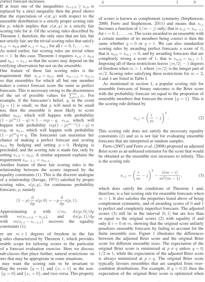
Table I. Scores si,j for negatively oriented fair scoring rules when m= 2,3and4. The constant,a, may be any number in[0,1/4].
m= 2 m= 3 m= 4 i j = 0 j= 1 j= 0 j = 1 j= 0 j= 1 0 0 1 0 1 0 1 1 0 0 0 1/3 0 1−3a 2 1 0 1/3 0 a a 3 1 0 1−3a 0 4 1 0
of scores is known as complement symmetry (Stephenson, 2000; Ferro and Stephenson, 2011) and means that si,j
becomes a function of|i/m−j|only; that issi,0=sm−i,1
fori= 0,1, . . . , m. The score awarded to an ensemble with a certain number of its members being correct is then the same whether y= 0 or y= 1. We can also standardize scoring rules by awarding perfect forecasts a score of 0, that iss0,0=sm,1= 0, and by awarding forecasts that are
completely wrong a score of 1, that is sm,0=s0,1= 1.
Imposing all of these restrictions leaves⌊m/2⌋ −1degrees of freedom whenm >1, where⌊m/2⌋is the integer part of m/2. Scoring rules satisfying these restrictions form= 2,
3and4are listed in Table I.
As mentioned in section 1, a popular scoring rule for ensemble forecasts of binary outcomes is the Brier score with the probability forecast set equal to the proportion of ensemble members that forecast the event{y= 1}. This is the scoring rule defined by
si,j= i m−j 2 . (2)
This scoring rule does not satisfy the necessary equality constraints (1) and so is not fair for evaluating ensemble forecasts that are interpreted as random samples.
Ferro (2007) and Ferro et al. (2008) proposed an adjusted Brier score as an unbiased estimator for the score that would be obtained as the ensemble size increases to infinity. This is the scoring rule
si,j = i m−j 2 − i(m−i) m2(m−1), (3)
which does satisfy the conditions of Theorem 1 and, therefore, is a fair scoring rule for ensemble forecasts when m >1. It also satisfies the properties listed above of being complement symmetric, and of awarding scores of0and1
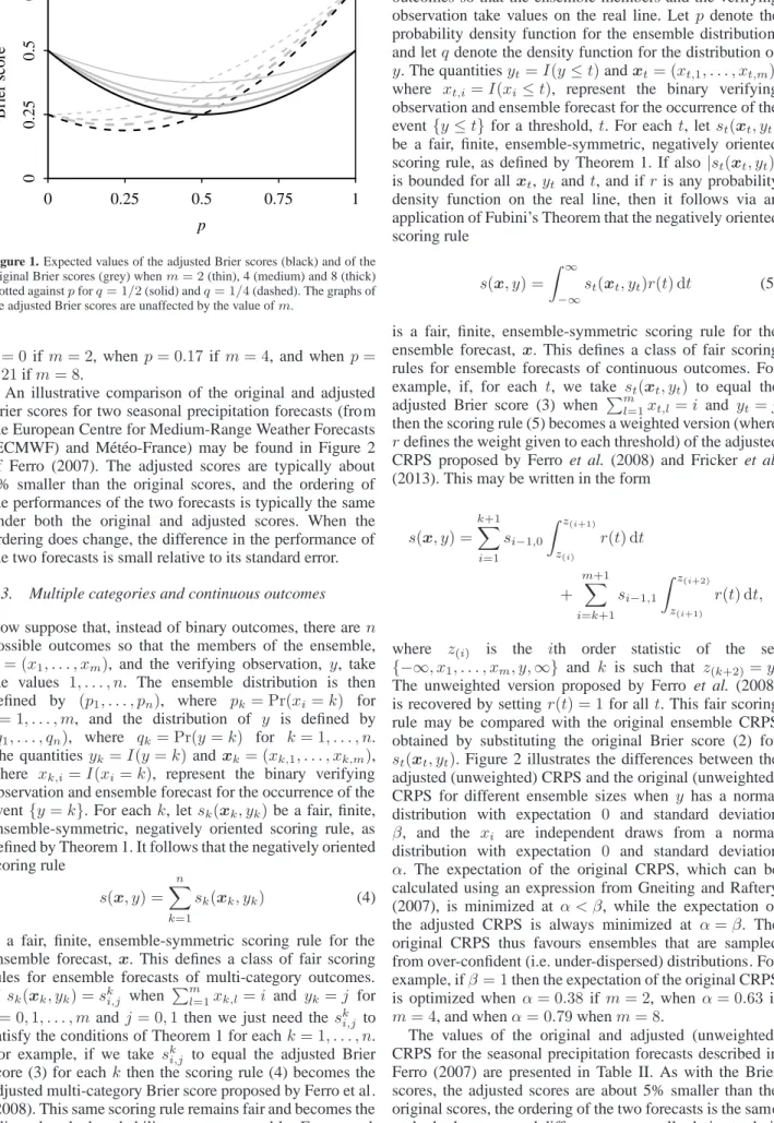
to perfect and completely imperfect forecasts. The adjusted scores (3) still lie in the interval [0,1] but are less than or equal to the original scores (2) with equality if and only ifi= 0orm, showing that the original score unfairly penalizes ensemble forecasts by failing to account for the finite ensemble size. Figure 1 illustrates the differences between the adjusted Brier score and the original Brier score for different ensemble sizes. The expectation of the original Brier score is minimized at p6=q unless q= 0,
1/2or1, while the expectation of the adjusted Brier score is always minimized at p=q. The original Brier score typically favours ensembles that are sampled from over-confident distributions. For example, if q= 0.25then the expectation of the original Brier score is optimized when
p Brier score 0 0.25 0.5 0.75 1 0 0.25 0.5 0.75
Figure 1. Expected values of the adjusted Brier scores (black) and of the original Brier scores (grey) whenm= 2(thin), 4 (medium) and 8 (thick) plotted againstpforq= 1/2(solid) andq= 1/4(dashed). The graphs of the adjusted Brier scores are unaffected by the value ofm.
p= 0if m= 2, whenp= 0.17if m= 4, and when p= 0.21ifm= 8.
An illustrative comparison of the original and adjusted Brier scores for two seasonal precipitation forecasts (from the European Centre for Medium-Range Weather Forecasts (ECMWF) and M´et´eo-France) may be found in Figure 2 of Ferro (2007). The adjusted scores are typically about 5% smaller than the original scores, and the ordering of the performances of the two forecasts is typically the same under both the original and adjusted scores. When the ordering does change, the difference in the performance of the two forecasts is small relative to its standard error.
2.3. Multiple categories and continuous outcomes Now suppose that, instead of binary outcomes, there aren possible outcomes so that the members of the ensemble, x= (x1, . . . , xm), and the verifying observation, y, take the values 1, . . . , n. The ensemble distribution is then defined by (p1, . . . , pn), where pk = Pr(xi=k) for
i= 1, . . . , m, and the distribution of y is defined by
(q1, . . . , qn), where qk = Pr(y=k) for k= 1, . . . , n.
The quantitiesyk =I(y=k)andxk= (xk,1, . . . , xk,m), where xk,i=I(xi=k), represent the binary verifying
observation and ensemble forecast for the occurrence of the event{y=k}. For eachk, letsk(xk, yk)be a fair, finite, ensemble-symmetric, negatively oriented scoring rule, as defined by Theorem 1. It follows that the negatively oriented scoring rule s(x, y) = n X k=1 sk(xk, yk) (4)
is a fair, finite, ensemble-symmetric scoring rule for the ensemble forecast, x. This defines a class of fair scoring rules for ensemble forecasts of multi-category outcomes. If sk(xk, yk) =ski,j when Pm
l=1xk,l=i and yk=j for
i= 0,1, . . . , mandj= 0,1 then we just need thesk i,j to
satisfy the conditions of Theorem 1 for eachk= 1, . . . , n. For example, if we take sk
i,j to equal the adjusted Brier
score (3) for eachkthen the scoring rule (4) becomes the adjusted multi-category Brier score proposed by Ferro et al. (2008). This same scoring rule remains fair and becomes the adjusted ranked probability score proposed by Ferro et al. (2008) if we redefineyk=I(y≤k)andxk,i=I(xi≤k).
Next, suppose that there is a continuum of scalar outcomes so that the ensemble members and the verifying observation take values on the real line. Let pdenote the probability density function for the ensemble distribution, and letqdenote the density function for the distribution of y. The quantitiesyt=I(y≤t)andxt= (xt,1, . . . , xt,m), where xt,i=I(xi≤t), represent the binary verifying
observation and ensemble forecast for the occurrence of the event{y≤t}for a threshold,t. For eacht, letst(xt, yt) be a fair, finite, ensemble-symmetric, negatively oriented scoring rule, as defined by Theorem 1. If also|st(xt, yt)| is bounded for all xt,ytandt, and ifris any probability density function on the real line, then it follows via an application of Fubini’s Theorem that the negatively oriented scoring rule
s(x, y) =
Z ∞
−∞
st(xt, yt)r(t) dt (5)
is a fair, finite, ensemble-symmetric scoring rule for the ensemble forecast, x. This defines a class of fair scoring rules for ensemble forecasts of continuous outcomes. For example, if, for each t, we take st(xt, yt) to equal the adjusted Brier score (3) when Pm
l=1xt,l=i and yt=j
then the scoring rule (5) becomes a weighted version (where rdefines the weight given to each threshold) of the adjusted CRPS proposed by Ferro et al. (2008) and Fricker et al. (2013). This may be written in the form
s(x, y) = k+1 X i=1 si−1,0 Z z(i+1) z(i) r(t) dt + m+1 X i=k+1 si−1,1 Z z(i+2) z(i+1) r(t) dt,
where z(i) is the ith order statistic of the set
{−∞, x1, . . . , xm, y,∞} and k is such that z(k+2)=y.
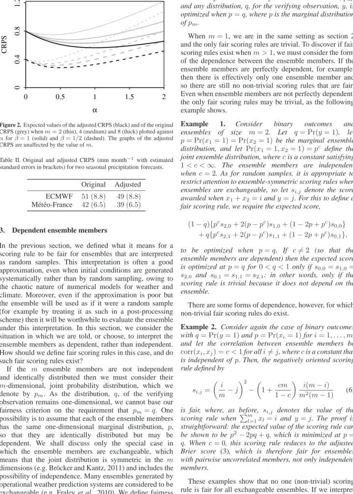
The unweighted version proposed by Ferro et al. (2008) is recovered by settingr(t) = 1for allt. This fair scoring rule may be compared with the original ensemble CRPS obtained by substituting the original Brier score (2) for st(xt, yt). Figure 2 illustrates the differences between the adjusted (unweighted) CRPS and the original (unweighted) CRPS for different ensemble sizes when y has a normal distribution with expectation 0 and standard deviation β, and the xi are independent draws from a normal
distribution with expectation 0 and standard deviation α. The expectation of the original CRPS, which can be calculated using an expression from Gneiting and Raftery (2007), is minimized at α < β, while the expectation of the adjusted CRPS is always minimized at α=β. The original CRPS thus favours ensembles that are sampled from over-confident (i.e. under-dispersed) distributions. For example, ifβ= 1then the expectation of the original CRPS is optimized whenα= 0.38 if m= 2, when α= 0.63 if m= 4, and whenα= 0.79whenm= 8.
The values of the original and adjusted (unweighted) CRPS for the seasonal precipitation forecasts described in Ferro (2007) are presented in Table II. As with the Brier scores, the adjusted scores are about 5% smaller than the original scores, the ordering of the two forecasts is the same under both scores, and differences are small relative to their standard errors.
α CRPS 0 0.5 1 1.5 2 0 0.4 0.8 1.2
Figure 2. Expected values of the adjusted CRPS (black) and of the original CRPS (grey) whenm= 2(thin), 4 (medium) and 8 (thick) plotted against αforβ= 1(solid) andβ= 1/2(dashed). The graphs of the adjusted CRPS are unaffected by the value ofm.
Table II. Original and adjusted CRPS (mm month−1 with estimated standard errors in brackets) for two seasonal precipitation forecasts.
Original Adjusted ECMWF 51 (8.8) 49 (8.8)
M´et´eo-France 42 (6.5) 39 (6.5)
3. Dependent ensemble members
In the previous section, we defined what it means for a scoring rule to be fair for ensembles that are interpreted as random samples. This interpretation is often a good approximation, even when initial conditions are generated systematically rather than by random sampling, owing to the chaotic nature of numerical models for weather and climate. Moreover, even if the approximation is poor but the ensemble will be used as if it were a random sample (for example by treating it as such in a post-processing scheme) then it will be worthwhile to evaluate the ensemble under this interpretation. In this section, we consider the situation in which we are told, or choose, to interpret the ensemble members as dependent, rather than independent. How should we define fair scoring rules in this case, and do such fair scoring rules exist?
If the m ensemble members are not independent and identically distributed then we must consider their m-dimensional, joint probability distribution, which we denote by pm. As the distribution, q, of the verifying
observation remains one-dimensional, we cannot base our fairness criterion on the requirement that pm=q. One
possibility is to assume that each of the ensemble members has the same one-dimensional marginal distribution, p, so that they are identically distributed but may be dependent. We shall discuss only the special case in which the ensemble members are exchangeable, which means that the joint distribution is symmetric in the m dimensions (e.g. Br¨ocker and Kantz, 2011) and includes the possibility of independence. Many ensembles generated by operational weather prediction systems are considered to be exchangeable (e.g. Fraley et al., 2010). We define fairness for exchangeable ensembles as follows.
Definition 4. A scoring rule, s(x, y), is fair for exchangeable ensembles,x, if its expectation with respect
to both the joint distribution of the ensemble members,pm,
and any distribution,q, for the verifying observation,y, is optimized whenp=q, wherepis the marginal distribution ofpm.
When m= 1, we are in the same setting as section 2 and the only fair scoring rules are trivial. To discover if fair scoring rules exist whenm >1, we must consider the form of the dependence between the ensemble members. If the ensemble members are perfectly dependent, for example, then there is effectively only one ensemble member and so there are still no non-trivial scoring rules that are fair. Even when ensemble members are not perfectly dependent, the only fair scoring rules may be trivial, as the following example shows.
Example 1. Consider binary outcomes and
ensembles of size m= 2. Let q= Pr(y= 1), let p= Pr(x1= 1) = Pr(x2= 1) be the marginal ensemble
distribution, and let Pr(x1= 1, x2= 1) =pc define the
joint ensemble distribution, wherecis a constant satisfying
1< c <∞. The ensemble members are independent when c= 2. As for random samples, it is appropriate to restrict attention to ensemble-symmetric scoring rules when ensembles are exchangeable, so let si,j denote the score
awarded whenx1+x2=iandy=j. For this to define a
fair scoring rule, we require the expected score,
(1−q){pcs
2,0+ 2(p−pc)s1,0+ (1−2p+pc)s0,0} +q{pcs
2,1+ 2(p−pc)s1,1+ (1−2p+pc)s0,1},
to be optimized when p=q. If c6= 2 (so that the ensemble members are dependent) then the expected score is optimized at p=q for 0< q <1 only ifs0,0=s1,0=
s2,0 and s0,1=s1,1=s2,1: in other words, only if the
scoring rule is trivial because it does not depend on the ensemble.
There are some forms of dependence, however, for which non-trivial fair scoring rules do exist.
Example 2. Consider again the case of binary outcomes
withq= Pr(y= 1)andp= Pr(xi = 1)fori= 1, . . . , m,
and let the correlation between ensemble members be
corr(xi, xj) =c <1for alli6=j, wherecis a constant that
is independent ofp. Then, the negatively oriented scoring rule defined by si,j= i m−j 2 − 1 + cm 1−c i(m−i) m2(m−1) (6)
is fair, where, as before, si,j denotes the value of the
scoring rule when Pm
l=1xl=i and y=j. The proof is
straightforward: the expected value of the scoring rule can be shown to be p2−2pq+q, which is minimized at p=
q. When c= 0, this scoring rule reduces to the adjusted Brier score (3), which is therefore fair for ensembles with pairwise uncorrelated members, not only independent members.
These examples show that no one (non-trivial) scoring rule is fair for all exchangeable ensembles. If we interpret an ensemble as exchangeable then we must specify its dependence structure and determine whether or not a fair scoring rule exists. If a fair scoring rule does exist then we should use it. If no fair scoring rule exists then an
alternative could be to use a scoring rule that is ‘nearly fair’ in some sense, for example a scoring rule whose expectation is optimized for a value ofpthat is always within a certain, small distance ofq. The development of this idea is left for future research.
In practice, the dependence structure of an ensemble is rarely stated by forecasters. This is problematic for verification given that we must specify a dependence structure in order to choose a fair scoring rule. Moreover, we cannot choose a fair scoring rule based on a dependence structure that has been estimated from the ensemble that is to be verified. For example, if we replacecwith an estimate in the scoring rule (6) of example 2 above then the scoring rule will no longer be fair. As a result, we shall rarely be able to specify the ‘correct’ dependence structure in our interpretation of an ensemble. This suggests disregarding the notion of a correct interpretation and instead verifying ensembles for one or more interpretations of interest. If it is likely that an ensemble will be used as if it were a random sample then it will be worthwhile verifying the ensemble using the fair scoring rules described in section 2. If it is likely that the empirical distribution function of an ensemble will be used as if it were a probability forecast then it will be worthwhile verifying the empirical distribution with proper scoring rules. We mentioned in section 2, however, that this latter interpretation is typically inappropriate.
4. Summary and discussion
A scoring rule for an ensemble forecast is fair if the expectation of the score with respect to the distributions of both the ensemble members and the verifying observation is optimized when these distributions coincide. Such scoring rules effectively evaluate the underlying distribution from which the ensemble members are sampled, and reward ensembles whose members behave as though they and the verifying observation are sampled from the same distribution.
When there is only one ensemble member, the only fair scoring rules are trivial. In this case, we should be aware that verification measures may favour ensembles that exhibit undesirable properties, such as being under-dispersed relative to the verifying observations (as in the example near the end of section 1). Fair scoring rules do exist when there is more than one ensemble member and they are independent and identically distributed. In this case, we have argued for the use of scoring rules that are symmetric in the ensemble members. In the case of binary outcomes, we have characterized a general class of fair scoring rules, which includes an adjusted version of the ensemble Brier score. We have also constructed classes of fair scoring rules for multi-category and continuous outcomes, which include adjusted versions of the ensemble ranked probability and continuous ranked probability scores. There is scope to extend these latter two classes to obtain more general characterizations of fair scoring rules for those forecasting situations.
Fair scoring rules can also exist when ensemble members are dependent, but the scoring rules are specific to the dependence structure and do not exist for some forms of dependence. Given that we are typically unable to specify the correct dependence structure of an ensemble, we recommend that ensembles are verified using scores that are fair for dependence structures of interest, including
independence. There is scope to compile a catalogue of fair scoring rules for different dependence structures.
Acknowledgements
This material is based upon work supported by the National Oceanic and Atmospheric Administration under Award No. NA12OAR4310085. The paper has benefitted from comments from Ian Jolliffe, Simon Mason, and three anonymous referees, one of whom helped to shorten the proof in the original manuscript.
Appendix
To prove Theorem 1, we need to find conditions on the scores si,j that make the scoring rule, s(x, y), fair. This is equivalent to making the expectation of the scoring rule with respect to the ensemble a proper scoring rule forp. As the ensemble members are independent withPr(xi= 1) =
1−Pr(xi= 0) =p, this expectation is sm(p, y) = m X i=0 m i pi(1−p)m−is i,y, (7)
and this is a regular scoring rule for p because |si,y|<
∞. Following Savage (1971), Gneiting and Raftery (2007) showed that any regular, negatively oriented scoring rule, s(p, y), is proper if and only if it can be written as
s(p, y) =G(p) + (y−p)G′
(p) (8)
for a concave functionGand whereG′
is the derivative of GifGis differentiable. (We have rewritten this result for negatively oriented, rather than positively oriented, scoring rules.) Forsto be strictly proper,Gmust be strictly concave. We seek conditions on si,j such that sm(p, y) has this
form (8).
Recall thatPr(y= 1) = 1−Pr(y= 0) =qand write sm(p, q) = m X i=0 m i pi(1−p)m−i {(1−q)si,0+qsi,1} and s(p, q) =G(p) + (q−p)G′ (p)
for the expectations ofsm(p, y)ands(p, y)with respect to
y. Evaluating these two expectations atq=pshows that we require G(p) = m X i=0 m i pi(1−p)m−i{(1−p)s i,0+psi,1}. (9) This also implies thatGmust be differentiable, so thatG′
is indeed the derivative ofG.
For sm(p, y) to be proper, we require sm(p, q) to be
minimized whenp=qfor all0≤q≤1. The derivative of sm(p, q)with respect top, when evaluated atp=q, can be
written as m X i=0 m i qi(1−q)m−i × {(m−i)(si+1,0−si,0)−i(si−1,1−si,1)}.
This equals zero for all 0< q <1 if and only if our equality constraints (1) hold. These constraints, therefore, are necessary conditions onsi,j.
Differentiating our expression (9) forG(p)yields G′ (p) = m X i=0 m i {(1−p)si,0+psi,1} d dpp i (1−p)m−i + m X i=0 m i pi(1−p)m−i(s i,1−si,0).
The first sum is the derivative ofsm(p, q)with respect to
p evaluated at q=p, and so is zero under our equality constraints, leaving G′ (p) = m X i=0 m i pi(1−p)m−i(s i,1−si,0). (10) It follows that G(p) + (y−p)G′ (p) =sm(p, y) so that
sm(p, y)has the correct form (8) and it remains to find
con-ditions onsi,jfor whichGis concave. Our expression (10)
forG′
is the difference in the expected scores when y= 1
andy= 0:G′
(p) =sm(p,1)−sm(p,0). If we letsi+1,0≥
si,0fori= 0,1, . . . , m−1then our equality constraints (1)
imply that si+1,1≤si,1 for i= 0,1, . . . , m−1 as well.
Under these inequality constraints, therefore, aspincreases, sm(p,1) decreases and sm(p,0) increases, so that G
′
(p)
decreases. In other words, G is concave, as required. If si+1,0> si,0for at least oneithenGis strictly concave. References
Anderson JL. 1996. A method for producing and evaluating probabilistic forecasts from ensemble model integrations. J. Clim. 9: 1518–1530. DOI: 10.1175/1520-0442(1996)009<1518:AMFPAE>2.0.CO;2. Brier GW. 1950. Verification of forecasts expressed in terms of
probability. Mon. Weather Rev. 78: 1–3. DOI: 10.1175/1520-0493(1950)078<0001:VOFEIT>2.0.CO;2.
Br¨ocker J. 2012. Evaluating raw ensembles with the continuous ranked probability score. Q. J. R. Meteorol. Soc. 138: 1611–1617. DOI: 10.1002/qj.1891.
Br¨ocker J, Kantz H. 2011. The concept of exchangeability in ensemble forecasting. Nonlinear Process. Geophys. 18: 1–5. DOI: 10.5194/npg-18-1-2011.
Br¨ocker J, Smith LA. 2007. Scoring probabilistic forecasts: the importance of being proper. Weather Forecast. 22: 382–388. DOI: WAF966.1.
Brown TA. 1974. ‘Admissible scoring systems for continuous distributions,’ Technical Note P-5235, 27pp. The Rand Corporation: Santa Monica, California, USA.
Ferro CAT. 2007. Comparing probabilistic forecasting systems with the Brier score. Weather Forecast. 22: 1076–1088. DOI: 10.1175/WAF1034.1.
Ferro CAT, Richardson DS, Weigel AP. 2008. On the effect of ensemble size on the discrete and continuous ranked probability scores. Meteorol. Appl. 15: 19–24. DOI: 10.1002/met.45.
Ferro CAT, Stephenson DB. 2011. Extremal dependence indices: improved verification measures for deterministic forecasts of rare binary events. Weather Forecast. 26: 699–713. DOI: WAF-D-10-05030.1.
Fraley C, Raftery AE, Gneiting T. 2010. Calibrating multimodel forecast ensembles with exchangeable and missing members using Bayesian model averaging. Mon. Weather Rev. 138: 190–202. DOI: 10.1175/2009MWR3046.1.
Fricker TE, Ferro CAT, Stephenson DB. 2013. Three recommendations for evaluating climate predictions. Meteorol. Appl. 20: 246–255. DOI: 10.1002/met.1409.
Gneiting T. 2011. Making and evaluating point forecasts. J. Am. Stat. Assoc. 106: 746–762. DOI: 10.1198/jasa.2011.r10138.
Gneiting T, Raftery AE. 2007. Strictly proper scoring rules, prediction, and estimation. J. Am. Stat. Assoc. 102: 359–378. DOI: 10.1198/016214506000001437.
Good IJ. 1952. Rational decisions. J. R. Stat. Soc. B 14: 107–114. Hamill TM, Colucci SJ. 1997. Verification of the Eta-RSM
short-range ensemble forecasts. Mon. Weather Rev. 125: 1312–1327. DOI: 10.1175/1520-0493(1997)125<1312:VOERSR>2.0.CO;2. Mason SJ, Galpin JS, Goddard L, Graham NE, Rajartnam B. 2007.
Conditional exceedance probabilities. Mon. Weather Rev. 135: 363– 372. DOI: 10.1175/MWR3284.1.
Mason SJ, Stephenson DB. 2008. ‘How do we know whether seasonal climate forecasts are any good?’ In Seasonal Climate: Forecasting and Managing Risk, Troccoli A, Harrison M, Anderson DLT, Mason SJ (eds). Springer: Dordrecht.
Mason SJ, Weigel AP. 2009. A generic forecast verification framework for administrative purposes. Mon. Weather Rev. 137: 331–349. DOI: 10.1175/2008MWR2553.1.
Matheson JE, Winkler RL. 1976. Scoring rules for continuous probability distributions. Management Science 22: 1087–1096. DOI: 10.1287/mnsc.22.10.1087.
McCarthy J. 1956. Measures of the value of information. Proc. Natl. Acad. Sci. 42: 654–655.
Murphy AH. 1997. ‘Forecast verification’. In Economic Value of Weather and Climate Forecasts, Katz RW, Murphy AH (eds). Cambridge University Press.
Murphy AH, Daan H. 1985. ‘Forecast evaluation’. In Probability, Statistics, and Decision Making in the Atmospheric Sciences, Murphy AH, Katz RW (eds). Westview Press: Boulder.
Savage LJ. 1971. Elicitation of personal probabilities and expectations. J. Am. Stat. Assoc. 66: 783–801. DOI: 10.1080/01621459.1971.10482346.
Stephenson DB. 2000. Use of the ‘odds ratio’ for diagnosing forecast skill. Weather Forecast. 15: 221–232. DOI: 10.1175/1520-0434(2000)015<0221:UOTORF>2.0.CO;2.
Stephenson DB, Doblas-Reyes FJ. 2000. Statistical methods for interpreting Monte Carlo ensemble forecasts. Tellus 52A: 300–322. DOI: 10.1034/j.1600-0870.2000.d01-5.x.
Weigel AP. 2012. ‘Verification of ensemble forecasts’. In Forecast Verification: a Practitioner’s Guide in Atmospheric Science, Jolliffe IT, Stephenson DB (eds). John Wiley and Sons: Chichester. Wilks DS. 2006. Statistical Methods in the Atmospheric Sciences. 2nd
ed. Academic Press: Amsterdam.
Winkler RL. 1967. The quantification of judgment: some method-ological suggestions. J. Am. Stat. Assoc. 62: 1105–1120. DOI: 10.1080/01621459.1967.10500920.
Winkler RL, Murphy AH. 1968. “Good” probability assessors. J. Appl. Meteorol. 7: 751–758. DOI: 10.1175/1520-0450(1968)007<0751:PA>2.0.CO;2.