Models for Longitudinal Data
Longitudinal data consist of repeated measurements on the same subject (or some other “experimental unit”) taken over time. Generally we wish to characterize the time trends within subjects and between subjects. The data will always include the response, the time covariate and the indicator of the subject on which the measurement has been made. If other covariates are recorded, say whether the subject is in the treatment group or the control group, we may wish to relate the within- and between-subject trends to such covariates.
In this chapter we introduce graphical and statistical techniques for the analysis of longitudinal data by applying them to a simple example.
4.1 The
sleepstudy
Data
Belenky et al. [2003] report on a study of the effects of sleep deprivation on reaction time for a number of subjects chosen from a population of long-distance truck drivers. These subjects were divided into groups that were allowed only a limited amount of sleep each night. We consider here the group of 18 subjects who were restricted to three hours of sleep per night for the first ten days of the trial. Each subject’s reaction time was measured several times on each day of the trial.
> str(sleepstudy)
'data.frame': 180 obs. of 3 variables:
$ Reaction: num 250 259 251 321 357 ...
$ Days : num 0 1 2 3 4 5 6 7 8 9 ...
$ Subject : Factor w/ 18 levels "308","309","310",..: 1 1 1 1 1 1 1 1 1..
In this data frame, the response variable Reaction, is the average of the reaction time measurements on a given subject for a given day. The two covariates areDays, the number of days of sleep deprivation, andSubject, the
Days of sleep deprivation
A
v
er
age reaction time (ms)
200 250 300 350 400 450 0 2 4 6 8 ● ● ● ● ● ●● ● ● ● 310 ● ● ● ● ●● ● ● ●● 309 0 2 4 6 8 ●● ● ● ● ● ● ● ● ● 370 ● ● ●● ● ●● ● ●● 349 0 2 4 6 8 ● ●● ● ● ● ● ● ● ● 350 ●● ●● ● ● ● ● ● ● 334 ●● ● ● ● ● ● ● ● ● 308 ● ● ●● ● ● ● ● ● ● 371 ● ● ● ● ● ● ● ● ● ● 369 ● ● ●●● ● ● ● ● ● 351 ● ● ●●● ● ● ● ● ● 335 200 250 300 350 400 450 ● ● ● ● ● ● ● ● ● ● 332 200 250 300 350 400 450 ● ● ●● ● ● ●● ● ● 372 0 2 4 6 8 ● ● ●● ● ● ●●● ● 333 ● ● ● ● ● ● ●● ●● 352 0 2 4 6 8 ● ●● ● ● ● ● ● ● ● 331 ● ● ● ● ●●● ● ● ● 330 0 2 4 6 8 ● ● ● ● ● ●● ● ● ● 337
Fig. 4.1 A lattice plot of the average reaction time versus number of days of sleep deprivation by subject for the sleepstudy data. Each subject’s data are shown in a separate panel, along with a simple linear regression line fit to the data in that panel. The panels are ordered, from left to right along rows starting at the bottom row, by increasing intercept of these per-subject linear regression lines. The subject number is given in the strip above the panel.
As recommended for any statistical analysis, we begin by plotting the data. The most important relationship to plot for longitudinal data on multiple subjects is the trend of the response over time by subject, as shown in Fig. 4.1. This plot, in which the data for different subjects are shown in separate panels with the axes held constant for all the panels, allows for examination of the time-trends within subjects and for comparison of these patterns between subjects. Through the use of small panels in a repeating pattern Fig. 4.1 conveys a great deal of information, the individual time trends for 18 subjects over 10 days — a total of 180 points — without being overly cluttered.
4.1.1 Characteristics of the
sleepstudy
Data Plot
The principles of “Trellis graphics”, developed by Bill Cleveland and his coworkers at Bell Labs and implemented in the lattice package for R by
Deepayan Sarkar, have been incorporated in this plot. As stated above, all the panels have the same vertical and horizontal scales, allowing us to eval-uate the pattern over time for each subject and also to compare patterns between subjects. The line drawn in each panel is a simple least squares line fit to the data in that panel only. It is provided to enhance our ability to discern patterns in both the slope (the typical change in reaction time per day of sleep deprivation for that particular subject) and the intercept (the average response time for the subject when on their usual sleep pattern).
The aspect ratio of the panels (ratio of the height to the width) has been chosen, according to an algorithm described in Cleveland [1993], to facilitate comparison of slopes. The effect of choosing the aspect ratio in this way is to have the slopes of the lines on the page distributed around ±45◦, thereby
making it easier to detect systematic changes in slopes.
The panels have been ordered (from left to right starting at the bottom row) by increasing intercept. Because the subject identifiers, shown in the strip above each panel, are unrelated to the response it would not be helpful to use the default ordering of the panels, which is by increasing subject number. If we did so our perception of patterns in the data would be confused by the, essentially random, ordering of the panels. Instead we use a characteristic of the data to determine the ordering of the panels, thereby enhancing our ability to compare across panels. For example, a question of interest to the experimenters is whether a subject’s rate of change in reaction time is related to the subject’s initial reaction time. If this were the case we would expect that the slopes would show an increasing trend (or, less likely, a decreasing trend) in the left to right, bottom to top ordering.
There is little evidence in Fig. 4.1 of such a systematic relationship between the subject’s initial reaction time and their rate of change in reaction time per day of sleep deprivation. We do see that for each subject, except 335, reaction time increases, more-or-less linearly, with days of sleep deprivation. However, there is considerable variation both in the initial reaction time and in the daily rate of increase in reaction time. We can also see that these data are balanced, both with respect to the number of observations on each subject, and with respect to the times at which these observations were taken. This can be confirmed by cross-tabulating Subject and Days.
> xtabs(~ Subject + Days, sleepstudy) Days Subject 0 1 2 3 4 5 6 7 8 9 308 1 1 1 1 1 1 1 1 1 1 309 1 1 1 1 1 1 1 1 1 1 310 1 1 1 1 1 1 1 1 1 1 330 1 1 1 1 1 1 1 1 1 1
331 1 1 1 1 1 1 1 1 1 1 332 1 1 1 1 1 1 1 1 1 1 333 1 1 1 1 1 1 1 1 1 1 334 1 1 1 1 1 1 1 1 1 1 335 1 1 1 1 1 1 1 1 1 1 337 1 1 1 1 1 1 1 1 1 1 349 1 1 1 1 1 1 1 1 1 1 350 1 1 1 1 1 1 1 1 1 1 351 1 1 1 1 1 1 1 1 1 1 352 1 1 1 1 1 1 1 1 1 1 369 1 1 1 1 1 1 1 1 1 1 370 1 1 1 1 1 1 1 1 1 1 371 1 1 1 1 1 1 1 1 1 1 372 1 1 1 1 1 1 1 1 1 1
In cases like this where there are several observations (10) per subject and a relatively simple within-subject pattern (more-or-less linear) we may want to examine coefficients from within-subject fixed-effects fits. However, because the subjects constitute a sample from the population of interest and we wish to drawn conclusions about typical patterns in the population and the subject-to-subject variability of these patterns, we will eventually want to fit mixed models and we begin by doing so. In section 4.4 we will com-pare estimates from a mixed-effects model with those from the within-subject fixed-effects fits.
4.2 Mixed-effects Models For the
sleepstudy
Data
Based on our preliminary graphical exploration of these data, we fit a mixed-effects model with two fixed-mixed-effects parameters, the intercept and slope of the linear time trend for the population, and two random effects for each subject. The random effects for a particular subject are the deviations in intercept and slope of that subject’s time trend from the population values.
We will fit two linear mixed models to these data. One model, fm8, allows
for correlation (in the unconditional distribution) of the random effects for the same subject. That is, we allow for the possibility that, for example, subjects with higher initial reaction times may, on average, be more strongly affected by sleep deprivation. The second model provides independent (again, in the unconditional distribution) random effects for intercept and slope for each subject.
4.2.1 A Model With Correlated Random Effects
The first model is fit as> (fm8 <- lmer(Reaction ~ 1 + Days + (1 + Days|Subject), sleepstudy,
+ REML = 0))
Linear mixed model fit by maximum likelihood
Formula: Reaction ~ 1 + Days + (1 + Days | Subject) Data: sleepstudy
AIC BIC logLik deviance
1764 1783 -876 1752
Random effects:
Groups Name Variance Std.Dev. Corr
Subject (Intercept) 565.516 23.7806
Days 32.682 5.7168 0.081
Residual 654.941 25.5918
Number of obs: 180, groups: Subject, 18 Fixed effects:
Estimate Std. Error t value
(Intercept) 251.405 6.632 37.91
Days 10.467 1.502 6.97
Correlation of Fixed Effects: (Intr)
Days -0.138
From the display we see that this model incorporates both an intercept and a slope (with respect to Days) in the fixed effects and in the random effects.
Extracting the conditional modes of the random effects
> head(ranef(fm8)[["Subject"]]) (Intercept) Days 308 2.815683 9.0755340 309 -40.048490 -8.6440671 310 -38.433156 -5.5133785 330 22.832297 -4.6587506 331 21.549991 -2.9445203 332 8.815587 -0.2352093
confirms that these are vector-valued random effects. There are a total of
q=36 random effects, two for each of the 18 subjects. The random effects section of the model display,
Groups Name Variance Std.Dev. Corr
Subject (Intercept) 565.516 23.7806
Days 32.682 5.7168 0.081
Residual 654.941 25.5918
indicates that there will be a random effect for the intercept and a random effect for the slope with respect to Days at each level of Subject and,
further-more, the unconditional distribution of these random effects, B∼N (0,Σ), allows for correlation of the random effects for the same subject.
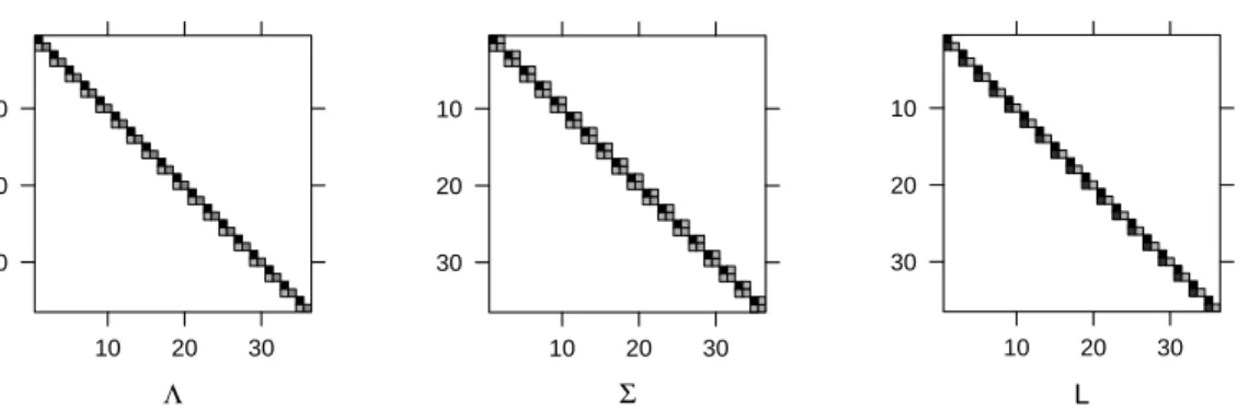
We can confirm the potential for correlation of random effects within sub-ject in the images ofΛ, Σ and L for this model (Fig. 4.2). The matrix Λ has
Λ 10 20 30 10 20 30 Σ 10 20 30 10 20 30 L 10 20 30 10 20 30
Fig. 4.2 Images ofΛ,Σ and Lfor model fm8
18 triangular blocks of size 2 along the diagonal, generating 18 square, sym-metric blocks of size 2 along the diagonal of Σ. The 18 symmetric blocks on the diagonal of Σ are identical. Overall we estimate two standard deviations and a correlation for a vector-valued random effect of size 2, as shown in the model summary.
Often the variances and the covariance of random effects are quoted, rather than the standard deviations and the correlation shown here. We have already seen that the variance of a random effect is a poor scale on which to quote the estimate because confidence intervals on the variance are so badly skewed. It is more sensible to assess the estimates of the standard deviations of random effects or, possibly, the logarithms of the standard deviations if we can be confident that 0 is outside the region of interest. We do display the estimates of the variances of the random effects but mostly so that the user can compare these estimates to those from other software or for cases where an estimate of a variance is expected (sometimes even required) to be given when reporting a mixed model fit.
We do not quote estimates of covariances of vector-valued random effects because the covariance is a difficult scale to interpret whereas a correlation has a fixed scale. A correlation must be between −1 and 1, allowing us to conclude that a correlation estimate close to those extremes indicates that Σ
is close to singular and the model is not well formulated.
The estimates of the fixed effects parameters are βb = (251.41,10.467)T. These represent a typical initial reaction time (i.e. without sleep deprivation) in the population of about 250 milliseconds, or 1/4 sec., and a typical in-crease in reaction time of a little more than 10 milliseconds per day of sleep deprivation.
The estimated subject-to-subject variation in the intercept corresponds to a standard deviation of about 25 ms. A 95% prediction interval on this random variable would be approximately±50ms. Combining this range with a population estimated intercept of 250 ms. indicates that we should not be
surprised by intercepts as low as 200 ms. or as high as 300 ms. This range is consistent with the reference lines shown in Figure 4.1.
Similarly, the estimated subject-to-subject variation in the slope corre-sponds to a standard deviation of about 6 ms./day so we would not be surprised by slopes as low as 10.5−2·5.7 =−0.9 ms./day or as high as
10.5+2·6=21.9 ms./day. Again, the conclusions from these rough, “back of the envelope” calculations are consistent with our observations from Fig. 4.1. The estimated residual standard deviation is about 25 ms. leading us to expect a scatter around the fitted lines for each subject of up to ±50 ms. From Figure 4.1 we can see that some subjects (309, 372 and 337) appear to have less variation than ±50 ms. about their within-subject fit but others (308, 332 and 331) may have more.
Finally, we see the estimated within-subject correlation of the random ef-fect for the intercept and the random efef-fect for the slope is very low, 0.081, confirming our impression that there is little evidence of a systematic rela-tionship between these quantities. In other words, observing a subject’s initial reaction time does not give us much information for predicting whether their reaction time will be strongly affected by each day of sleep deprivation or not. It seems reasonable that we could get nearly as good a fit from a model that does not allow for correlation, which we describe next.
4.2.2 A Model With Uncorrelated Random Effects
In a model with uncorrelated random effects we have B ∼N (0,Σ) where
Σ is diagonal. We have seen models like this in previous chapters but those models had simple scalar random effects for all the grouping factors. Here we want to have a simple scalar random effect for Subject and a random effect
for the slope with respect to Days, also indexed by Subject. We accomplish
this by specifying two random-effects terms. The first,(1|Subject), is a simple scalar term. The second has Days on the left hand side of the vertical bar.
It seems that the model formula we want should be
Reaction ~ 1 + Days + (1 | Subject) + (Days | Subject)
but it is not. Because the intercept is implicit in linear models, the second ran-dom effects term is equivalent to(1+Days|Subject) and will, by itself, produce correlated, vector-valued random effects.
We must suppress the implicit intercept in the second random-effects term which we do by writing it as (0+Days|Subject), read as “no intercept and
Days by Subject”. An alternative expression for Days without an intercept by Subject is (Days - 1 | Subject). Using the first form we have
> (fm9 <- lmer(Reaction ~ 1 + Days + (1|Subject) + (0+Days|Subject),
Linear mixed model fit by maximum likelihood
Formula: Reaction ~ 1 + Days + (1 | Subject) + (0 + Days | Subject) Data: sleepstudy
AIC BIC logLik deviance
1762 1778 -876 1752
Random effects:
Groups Name Variance Std.Dev.
Subject (Intercept) 584.249 24.1713
Subject Days 33.633 5.7994
Residual 653.116 25.5561
Number of obs: 180, groups: Subject, 18 Fixed effects:
Estimate Std. Error t value
(Intercept) 251.405 6.708 37.48
Days 10.467 1.519 6.89
Correlation of Fixed Effects: (Intr)
Days -0.194
As in model fm8, there are two random effects for each subject
> head(ranef(fm9)[["Subject"]]) (Intercept) Days 308 1.854653 9.2364353 309 -40.022293 -8.6174753 310 -38.723150 -5.4343821 330 23.903313 -4.8581932 331 22.396316 -3.1048397 332 9.051998 -0.2821594
but no correlation has been estimated
Groups Name Variance Std.Dev.
Subject (Intercept) 584.249 24.1713
Subject Days 33.633 5.7994
Residual 653.116 25.5561
The Subject factor is repeated in the “Groups” column because there were
two distinct terms generating these random effects and these two terms had the same grouping factor.
Images of the matrices Λ, Σ and L (Fig. 4.3) show thatΣ is indeed diago-nal. The order of the random effects inΣ andΛ for modelfm9is different from
the order in model fm8. In model fm8 the two random effects for a particular
subject were adjacent. In model fm9 all the intercept random effects occur
first then all the Days random effects. The sparse Cholesky decomposition,
L, has the same form in both models because the fill-reducing permutation (described in Sect. 5.4.1) calculated for model fm9 provides a post-ordering
to group random effects with similar structure in Z.
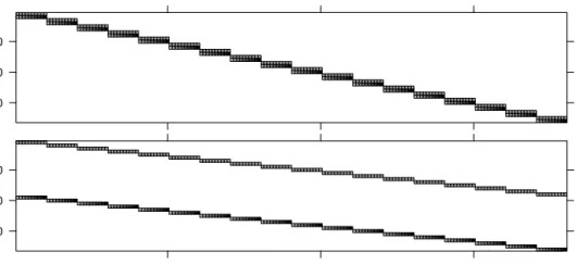
Images of ZT for these two models (Fig. 4.4) shows that the columns of Z
(rows of ZT) from one model are the same those from the other model but
Λ 10 20 30 10 20 30 Σ 10 20 30 10 20 30 L 10 20 30 10 20 30
Fig. 4.3 Images ofΛ, the relative covariance factor, Σ, the variance-covariance ma-trix of the random effects, and L, the sparse Cholesky factor, in model fm9
10 20 30 10 20 30
Fig. 4.4 Images of ZT for models fm8 (upper panel) and fm9 (lower panel)
4.2.3 Generating
Z
and
Λ
From Random-effects Terms
Let us consider these columns in more detail, starting with the columns of Z for model fm9. The first 18 columns (rows in the bottom panel of Fig. 4.4)
are the indicator columns for theSubjectfactor, as we would expect from the simple, scalar random-effects term(1|Subject). The pattern of zeros and
non-zeros in the second group of 18 columns is determined by the indicators of the grouping factor, Subject, and the values of the non-zeros are determined by the Days factor. In other words, these columns are formed by the interaction
of the numeric covariate, Days, and the categorical covariate, Subject.
The non-zero values in the model matrix Z for model fm8 are the same as
those for modelfm8 but the columns are in a different order. Pairs of columns
associated with the same level of the grouping factor are adjacent. One way to think of the process of generating these columns is to extend the idea of an
interaction between a single covariate and the grouping factor to generating an “interaction” of a model matrix and the levels of the grouping factor. In other words, we begin with the two columns of the model matrix for the expression 1 + Days and the 18 columns of indicators for the Subject factor. The result will have 36 columns that are considered as 18 adjacent pairs. The values within each of these pairs of columns are the values of the 1 + Days
columns, when the indicator is 1, otherwise they are zero.
We can now describe the general process of creating the model matrix, Z, and the relative covariance factor, Λ from the random-effects terms in the model formula. Each random-effects term is of the form (expr|fac). The
expression expr is evaluated as a linear model formula, producing a model
matrix with s columns. The expression fac is evaluated as a factor. Let k
be the number of levels in this factor, after eliminating unused levels, if any. The ith term generates siki columns in the model matrix, Z, and a diagonal
block of size siki in the relative covariance factor, Λ. The siki columns in Z
have the pattern of the interaction of the si columns from the ith expr with
the k indicator columns for the factor fac. The diagonal block in Λ is itself
block diagonal, consisting of ki blocks, each a lower triangular matrix of size
si. In fact, these inner blocks are repetitions of the same lower triangular
si×si matrix. The i term contributes si(si+1)/2 elements to the
variance-component parameter, θ, and these are the elements in the lower triangle of this si×si template matrix.
Note that when counting the columns in a model matrix we must take into account the implicit intercept term. For example, we could write the formula for model fm8 as
Reaction ~ Days + (Days | Subject)
realizing that the linear model expression, Days, actually generates two columns because of the implicit intercept.
Whether or not to include an explicit intercept term in a model formula is a matter of personal taste. Many people prefer to write the intercept explicitly in the formula so as to emphasize the relationship between terms in the formula and coefficients or random effects in the model. Others omit these implicit terms so as to economize on the amount of typing required. Either approach can be used. The important point to remember is that the intercept must be explicitly suppressed when you don’t want it in a term.
Also, the intercept term must be explicit when it is the only term in the expression. That is, a simple, scalar random-effects term must be written as
(1|fac) because a term like (|fac) is not syntactically correct. However, we
can omit the intercept from the fixed-effects part of the model formula if we have any random-effects terms. That is, we could write the formula for model
fm1 in Chap. 1 as
Yield ~ (1 | Batch)
Yield ~ 1 | Batch
although omitting the parentheses around a random-effects term is risky. Because of operator precedence, the vertical bar operator, |, takes essentially
everything in the expression to the left of it as its first operand. It is advisable always to enclose such terms in parentheses so the scope of the operands to the | operator is clearly defined.
4.2.4 Comparing Models
fm9and
fm8Returning to models fm8 and fm9 for the sleepstudy data, it is easy to see that these are nested models because fm8 is reduced to fm9 by constraining
the within-group correlation of random effects to be zero (which is equivalent to constraining the element below the diagonal in the 2×2 lower triangular blocks ofΛ in Fig. 4.2 to be zero).
We can use a likelihood ratio test to compare these fitted models.
> anova(fm9, fm8) Data: sleepstudy Models:
fm9: Reaction ~ 1 + Days + (1 | Subject) + (0 + Days | Subject) fm8: Reaction ~ 1 + Days + (1 + Days | Subject)
Df AIC BIC logLik Chisq Chi Df Pr(>Chisq)
fm9 5 1762.0 1778.0 -876.00
fm8 6 1763.9 1783.1 -875.97 0.0639 1 0.8004
The value of the χ2 statistic,0.0639, is very small, corresponding to a p-value
of 0.80 and indicating that the extra parameter in model fm8 relative to fm9
does not produce a significantly better fit. By the principal of parsimony we prefer the reduced model, fm9.
This conclusion is consistent with the visual impression provided by Fig. 4.1. There does not appear to be a strong relationship between a sub-ject’s initial reaction time and the extent to which his or her reaction time is affected by sleep deprivation.
In this likelihood ratio test the value of the parameter being tested, a correlation of zero, is not on the boundary of the parameter space. We can be confident that the p-value from the LRT adequately reflects the underlying situation.
(Note: It is possible to extend profiling to the correlation parameters and we will do so but that has not been done yet.)
4.3 Assessing the Precision of the Parameter Estimates
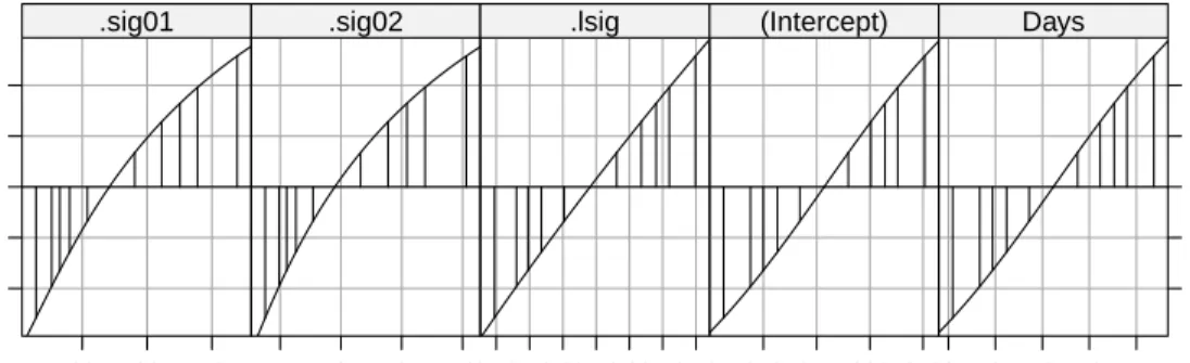
Plots of the profile ζ for the parameters in model fm9 (Fig. 4.5)show thatζ −2 −1 0 1 2 20 30 40 .sig01 4 6 8 10 .sig02 3.10 3.20 3.30 3.40 .lsig 240 250 260 270 (Intercept) 6 8 10 12 14 Days
Fig. 4.5 Profile zeta plot for each of the parameters in modelfm9. The vertical lines are the endpoints of 50%, 80%, 90%, 95% and 99% profile-based confidence intervals for each parameter.
confidence intervals onσ1 andσ2 will be slightly skewed; those forlog(σ) will
be symmetric and well-approximated by methods based on quantiles of the standard normal distribution and those for the fixed-effects parameters, β1
and β2 will be symmetric and slightly over-dispersed relative to the standard
normal. For example, the 95% profile-based confidence intervals are
> confint(pr9) 2.5 % 97.5 % .sig01 15.258637 37.786532 .sig02 3.964074 8.769159 .lsig 3.130287 3.359945 (Intercept) 237.572148 265.238062 Days 7.334067 13.600505
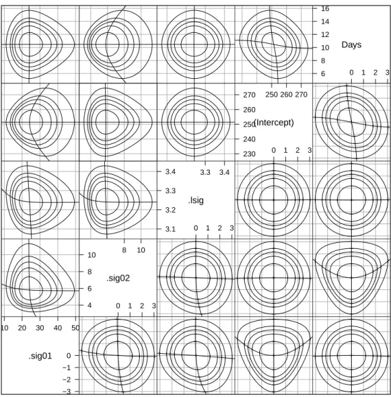
The profile pairs plot (Fig. 4.6) shows, for the most part, the usual pat-terns. First, consider the panels below the diagonal, which are on the (ζi,ζj)
scales. The ζ pairs for log(σ) and β0, in the (4,3) panel, and for log(σ) and
β1, in the (5,3) panel, show the ideal pattern. The profile traces are straight
and orthogonal, producing interpolated contours on theζ scale that are con-centric circles centered at the origin. When mapped back to the scales of
log(σ) and β0 or β1, in panels (3,4) and (3,5), these circles become slightly
distorted, but this is only due to the moderate nonlinearity in the profile ζ
plots for these parameters.
Examining the profile traces on the ζ scale for log(σ) versus σ1, the (3,1)
panel, or versus σ2, the (3,2) panel, and for σ1 versus σ2, the (2,1) panel,
we see that close to the estimate the traces are orthogonal but as one vari-ance component becomes small there is usually an increase in the others. In some sense the total variability in the response will be partitioned across the contribution of the fixed effects and the variance components. In each of
Scatter Plot Matrix .sig01 10 20 30 40 50 −3 −2 −1 0 .sig02 4 6 8 10 8 10 0 1 2 3 .lsig 3.1 3.2 3.3 3.4 3.3 3.4 0 1 2 3 (Intercept) 230 240 250 260 270 250 260 270 0 1 2 3 Days 6 8 10 12 14 16 0 1 2 3
Fig. 4.6 Profile pairs plot for the parameters in model fm9. The contour lines cor-respond to marginal 50%, 80%, 90%, 95% and 99% confidence regions based on the likelihood ratio. Panels below the diagonal represent the (ζi,ζj) parameters; those above the diagonal represent the original parameters.
these panels the fixed-effects parameters are at their optimal values, condi-tional on the values of the variance components, and the variance components must compensate for each other. If one is made smaller then the others must become larger to compensate.
The patterns in the (4,1) panel (σ1 versusβ0, on theζ scale) and the (5,2)
panel (σ2 versus β1, on theζ scale) are what we have come to expect. As the
fixed-effects parameter is moved from its estimate, the standard deviation of the corresponding random effect increases to compensate. The (5,1) and (4,2) panels show that changing the value of a fixed effect doesn’t change the estimate of the standard deviation of the random effects corresponding to
the other fixed effect, which makes sense although the perfect orthogonality shown here will probably not be exhibited in models fit to unbalanced data. In some ways the most interesting panels are those for the pair of fixed-effects parameters: (5,4) on the ζ scale and (4,5) on the original scale. The traces are not orthogonal. In fact the slopes of the traces at the origin of the (5,4) (ζ scale) panel are the correlation of the fixed-effects estimators
(−0.194 for this model) and its inverse. However, as we move away from
the origin on one of the traces in the (5,4) panel it curves back toward the horizontal axis (for the horizontal trace) or the vertical axis (for the vertical trace). In the ζ scale the individual contours are still concentric ellipses but their eccentricity changes from contour to contour. The innermost contours have greater eccentricity than the outermost contours. That is, the outermost contours are more like circles than are the innermost contours.
In a fixed-effects model the shapes of projections of deviance contours onto pairs of fixed-effects parameters are consistent. In a fixed-effects model the profile traces in the original scale will always be straight lines. For mixed models these traces can fail to be linear, as we see here, contradicting the widely-held belief that inferences for the fixed-effects parameters in linear mixed models, based on T or F distributions with suitably adjusted degrees of freedom, will be completely accurate. The actual patterns of deviance contours are more complex than that.
4.4 Examining the Random Effects and Predictions
The result of applying ranef to fitted linear mixed model is a list of data
frames. The components of the list correspond to the grouping factors in the random-effects terms, not to the terms themselves. Model fm9 is the first
model we have fit with more than one term for the same grouping factor where we can see the combination of random effects from more than one term.
> str(rr1 <- ranef(fm9)) List of 1
$ Subject:'data.frame': 18 obs. of 2 variables:
..$ (Intercept): num [1:18] 1.85 -40.02 -38.72 23.9 22.4 ...
..$ Days : num [1:18] 9.24 -8.62 -5.43 -4.86 -3.1 ...
- attr(*, "class")= chr "ranef.mer"
Theplot method for"ranef.mer" objects produces one plot for each grouping
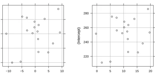
factor. For scalar random effects the plot is a normal probability plot. For two-dimensional random effects, including the case of two scalar terms for the same grouping factor, as in this model, the plot is a scatterplot. For three or more random effects per level level of the grouping factor, the plot is a scatterplot matrix. The left hand panel in Fig. 4.7 was created with
Days (Intercept) −40 −20 0 20 −10 −5 0 5 10 ● ● ● ● ● ● ● ● ● ● ● ● ● ● ● ● ● ● Days (Intercept) 220 240 260 280 0 5 10 15 20 ● ● ● ● ● ● ● ● ● ● ● ● ● ● ● ● ● ●
Fig. 4.7 Plot of the conditional modes of the random effects for model fm9 (left panel) and the corresponding subject-specific coefficients (right panel)
The coef method for a fitted lmer model combines the fixed-effects esti-mates and the conditional modes of the random effects, whenever the column names of the random effects correspond to the names of coefficients. For model
fm9 the fixed-effects coefficients are (Intercept) and Days and the columns of
the random effects match these names. Thus we can calculate some kind of per-subject “estimates” of the slope and intercept and plot them, as in the right hand panel of Fig. 4.7. By comparing the two panels in Fig. 4.7 we can see that the result of thecoef method is simply the conditional modes of the random effects shifted by the coefficient estimates.
It is not entirely clear how we should interpret these values. They are a combination of parameter estimates with the modal values of random vari-ables and, as such, are in a type of “no man’s land” in the probability model. (In the Bayesian approach [Box and Tiao, 1973] to inference, however, both the parameters and the random effects are random variables and the pretation of these values is straightforward.) Despite the difficulties of inter-pretation in the probability model, these values are of interest because they determine the fitted response for each subject.
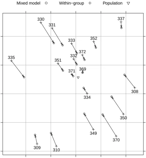
Because responses for each individual are recorded on each of ten days we can determine the within-subject estimates of the slope and intercept (that is, the slope and intercept of each of the lines in Fig. 4.1). In Fig. 4.8 we compare the within-subject least squares estimates to the per-subject slope and intercept calculated from model fm9. We see that, in general, the
per-subject slopes and intercepts from the mixed-effects model are closer to the population estimates than are the within-subject least squares estimates. This pattern is sometimes described as a shrinkage of coefficients toward the population values.
Days (Intercept) 200 220 240 260 280 0 5 10 15 20 ● ● ● ● ● ● ● ● ● ● ● ● ● ● ● ● ● ● 308 309 310 334 349 350 370 330 331 332 333 335 337 351 352 369 371 372
Mixed model ● Within−group Population
Fig. 4.8 Comparison of the within-subject estimates of the intercept and slope for each subject and the conditional modes of the per-subject intercept and slope. Each pair of points joined by an arrow are the within-subject and conditional mode esti-mates for the same subject. The arrow points from the within-subject estimate to the conditional mode for the mixed-effects model. The subject identifier number is at the head of each arrow.
The term “shrinkage” may have negative connotations. John Tukey pre-ferred to refer to the process as the estimates for individual subjects “bor-rowing strength” from each other. This is a fundamental difference in the models underlying mixed-effects models versus strictly fixed-effects models. In a mixed-effects model we assume that the levels of a grouping factor are a selection from a population and, as a result, can be expected to share charac-teristics to some degree. Consequently, the predictions from a mixed-effects model are attenuated relative to those from strictly fixed-effects models.
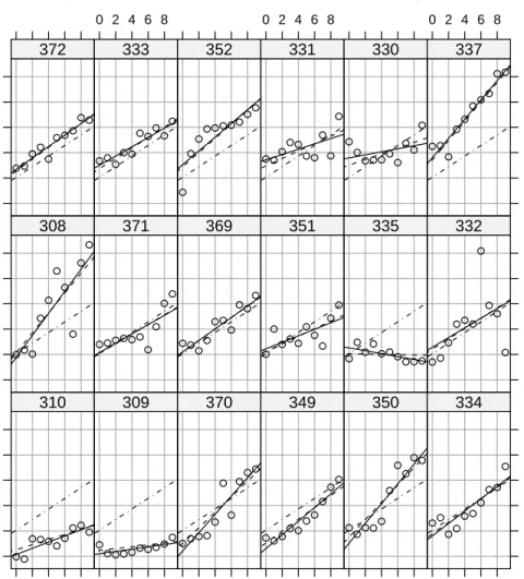
The predictions from model fm9 and from the within-subject least squares fits for each subject are shown in Fig. 4.9. In may seem that the shrinkage
Days of sleep deprivation
A
v
er
age reaction time (ms)
200 250 300 350 400 450 0 2 4 6 8 ● ● ● ● ●●●● ● ● 310 ● ● ● ● ●● ● ● ●● 309 0 2 4 6 8 ●● ● ● ● ● ● ●● ● 370 ● ●●● ● ●● ● ●● 349 0 2 4 6 8 ● ●● ● ● ● ● ● ● ● 350 ●● ●● ● ● ● ● ● ● 334 ●● ● ● ● ● ● ● ● ● 308 ● ● ●● ● ● ● ● ● ● 371 ● ● ● ● ● ● ● ● ●● 369 ● ● ●●● ● ● ● ● ● 351 ● ● ●●● ● ● ● ● ● 335 200 250 300 350 400 450 ● ● ● ● ● ● ● ● ● ● 332 200 250 300 350 400 450 ● ● ●● ● ● ●● ● ● 372 0 2 4 6 8 ● ● ●● ● ● ●●● ● 333 ● ● ● ● ● ● ●● ●● 352 0 2 4 6 8 ● ●● ● ● ● ● ● ● ● 331 ● ● ● ● ●●● ● ● ● 330 0 2 4 6 8 ● ● ● ● ● ●● ● ● ● 337 Within−subject Mixed model Population
Fig. 4.9 Comparison of the predictions from the within-subject fits with those from the conditional modes of the subject-specific parameters in the mixed-effects model. from the per-subject estimates toward the population estimates depends only on how far the per-subject estimates (solid lines) are from the population es-timates (dot-dashed lines). However, careful examination of this figure shows that there is more at work here than a simple shrinkage toward the popula-tion estimates proporpopula-tional to the distance of the per-subject estimates from the population estimates.
It is true that the mixed model estimates for a particular subject are “between” the within-subject estimates and the population estimates, in the sense that the arrows in Fig. 4.8 all point somewhat in the direction of the population estimate. However, the extent of the attenuation of the within-subject estimates toward the population estimates is not simply related to the distance between those two sets of estimates. Consider the two panels, labeled 330 and 337, at the top right of Fig. 4.9. The within-subject estimates for 337
are quite unlike the population estimates but the mixed-model estimates are very close to these within-subject estimates. That is, the solid line and the dashed line in that panel are nearly coincident and both are a considerable distance from the dot-dashed line. For subject 330, however, the dashed line is more-or-less an average of the solid line and the dot-dashed line, even though the solid and dot-dashed lines are not nearly as far apart as they are for subject 337.
The difference between these two cases is that the within-subject estimates for 337 are very well determined. Even though this subject had an unusually large intercept and slope, the overall pattern of the responses is very close to a straight line. In contrast, the overall pattern for 330 is not close to a straight line so the within-subject coefficients are not well determined. The multiple
R2 for the solid line in the 337 panel is 93.3% but in the 330 panel it is only
15.8%. The mixed model can pull the predictions in the 330 panel, where the data are quite noisy, closer to the population line without increasing the residual sum of squares substantially. When the within-subject coefficients are precisely estimated, as in the 337 panel, very little shrinkage takes place. We see from Fig. 4.9 that the mixed-effects model smooths out the between-subject differences in the predictions by bringing them closer to a common set of predictions, but not at the expense of dramatically increasing the sum of squared residuals. That is, the predictions are determined so as to balance fidelity to the data, measured by the residual sum of squares, with simplicity of the model. The simplest model would use the same prediction in each panel (the dot-dashed line) and the most complex model, based on linear relationships in each panel, would correspond to the solid lines. The dashed lines are between these two extremes. We will return to this view of the predictions from mixed models balancing complexity versus fidelity in Sec. 5.3, where we make the mathematical nature of this balance explicit.
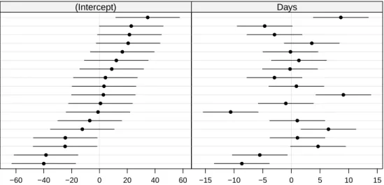
We should also examine the prediction intervals on the random effects (Fig. 4.10) where we see that many prediction intervals overlap zero but there are several that do not.. In this plot the subjects are ordered from bottom to top according to increasing conditional mode of the random effect for(Intercept). The resulting pattern in the conditional modes of the random effect for Days reinforces our conclusion that the model fm9, which does not
allow for correlation of the random effects for(Intercept)andDays, is suitable.
4.5 Chapter Summary
Problems
4.1. Check the structure of documentation, structure and a summary of the
309 310 370 349 350 334 335 371 308 369 351 332 372 333 352 331 330 337 −60 −40 −20 0 20 40 60 ● ● ● ● ● ● ● ● ● ● ● ● ● ● ● ● ● ● (Intercept) −15 −10 −5 0 5 10 15 ● ● ● ● ● ● ● ● ● ● ● ● ● ● ● ● ● ● Days
Fig. 4.10 Prediction intervals on the random effects for model fm9.
(a) Create anxyplotof the distance versusage bySubject for the female
sub-jects only. You can use the optional argument subset = Sex == "Female"
in the call to xyplot to achieve this. Use the optional argument type = c("g","p","r") to add reference lines to each panel.
(b) Enhance the plot by choosing an aspect ratio for which the typical slope of the reference line is around 45o. You can set it manually (something like aspect = 4) or with an automatic specification (aspect = "xy"). Change the layout so the panels form one row (layout = c(11,1)).
(c) Order the panels according to increasing response at age 8. This is achieved with the optional argument index.cond which is a function of
arguments x and y. In this case you could use index.cond = function(x,y) y[x == 8]. Add meaningful axis labels. Your final plot should be like
Age (yr)
Distance from pituitar
y to pter ygomaxillar y fissure (mm) 16 18 20 22 24 26 28 8 9 11 13 ● ● ● ● F10 8 9 11 13 ● ● ● ● F06 8 9 11 13 ● ● ● ● F09 8 9 11 13 ● ● ● ● F03 8 9 11 13 ● ● ● ● F01 8 9 11 13 ● ● ● ● F02 8 9 11 13 ● ● ● ● F05 8 9 11 13 ● ● ● ● F07 8 9 11 13 ● ● ● ● F08 8 9 11 13 ● ● ● ● F04 8 9 11 13 ● ● ● ● F11
(d) Fit a linear mixed model to the data for the females only with random effects for the intercept and for the slope by subject, allowing for corre-lation of these random effects within subject. Relate the fixed effects and the random effects’ variances and covariances to the variability shown in the figure.
(e) Produce a “caterpillar plot” of the random effects for intercept and slope. Does the plot indicate correlated random effects?
(f) Consider what the Intercept coefficient and random effects represents. What will happen if you center the ages by subtracting 8 (the baseline year) or 11 (the middle of the age range)?
(g) Repeat for the data from the male subjects.
4.2.
Fit a model to both the female and the male subjects in the Orthodont data
set, allowing for differences by sex in the fixed-effects for intercept (probably with respect to the centered age range) and slope.