Why is Child Labor Illegal?
Sylvain Dessy and John Knowles
∗May 2001
Abstract
We argue from an empirical analysis of Latin-American household surveys that per capita income in the country of residence has a negative effect on child labor supply,
even after controlling for other household characteristics. We then develop a theory of the emergence of mandatory-education laws. If parents are unable to commit to
educating their children, child-labor laws can increase the welfare of altruistic parents in an ex ante sense. The theory suggests that measures that reduce child wages can make poor families better off, but that this may come at the expense of even poorer
families.
JEL Classification: D31, I21, J22 O12.
Key Words: Child Labor Legislation, Economic Development.
∗Affiliations: Dessy, Dept. des Sciences Economiques, Universite Laval, Quebec, Qc,Canada
[[email protected]]; Knowles, Dept. of Economics, University of Pennsylvania, 3718 Locust Walk, Philadel-phia, PA 19104[[email protected]]. The authors thank Miguel Szekely and Alejandro Gaviria of the InterAmerican Development Bank, as well as the statistical agencies of Argentina, Bolivia, Brasil, Chile, Colombia, Costa Rica, Ecuador, Mexico, Panama, Paraguay, Peru and Venezuela for access to household survey data. We are also grateful to Bernard Fortin, and Steven Gordon for helpful discussions, and to sem-inar participants at the NBER Summer Institute 2000, SED 2000, and ITAM’s “Consequences of Financial Crises” conference, Summer 2000. Knowles is grateful forfinancial support from the NSF.
1. Introduction
Until a little more than 150 years ago, child labor was the rule among poor children in most countries, including the US and Great Britain. Today, many countries have laws banning or restricting child labor. The ILO convention C138 against child labor has been ratified by 89 countries, indicating opposition to child labor generally among these countries. Yet it is not clear from the current state of economic theory why full-time education of children should be compulsory. Indeed, given standard versions of the economic theory of the household, as in Becker (1976) and Rosenzweig and Evenson (1977), in which altruistic parents only send their children to work when this enhances the welfare of the family, laws against child labor can only reduce the welfare of households, particularly those so poor that children’s income is essential for survival.1
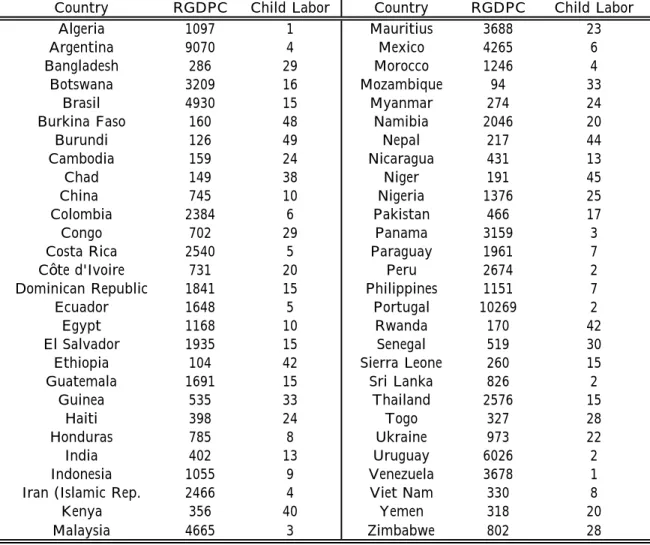
Under standard assumptions, the simplest explanation of the above observations is that child labor laws are not binding; they merely formalize the optimal decisions of households in countries that have become so rich over time that even the poorest parents want to educate their children. In Figure 1, we present the results of a regression for 54 countries for which the UN has reported positive child-labor rates for 1998. The graph suggests that child labor around the world is negatively related to GDP per capita. In fact, variation in GDP explains 1As today in poor countries, the children of poor parents were likely to spend little time in education and
instead work in paid employment outside the home, or in a family business, such as agriculture or a cottage industry. Equivalently, children were also likely to devote their time to domestic work, enabling parents to spend more time in labor outside the home. In India today, Anker and Melkas (1996) has estimated that children’s contributions to the household often constitute as much as 25% of the household’s income, per child.
Grootaert and Kanbur (1995) show that only after the incidence of child labor had already begun to decline, in 1833, a time when 36.6 % of boys aged 10-14 were working, did Britain pass legislation restricting child labor. This, as well as the observation by Goldin (1979) that higher wages for fathers in Philadelphia in the late 19th century reduced the probability of child labor, suggest that the forces driving child labor in poor countries today are fundamentally similar to those experienced by the US and England in the 19th century.
68% of the variance in child-labor rates among these countries.2
This raises two questions. First, are child labor and education laws really responsible for reducing child labor? If the answer to this question is affirmative, the second question is why such laws are enacted. Of course it is always possible to explain such laws by appealing to externalities in the labor market, or to inter-dependent preferences, but the question is whether there is a simple explanation, closer to standard theory, that yields empirically falsifiable predictions about the emergence of restrictions on child labor?
It is not obvious how to answer the first question, because there do not exist simple measures of the status of child labor by country. There are several reasons for this difficulty. First there are many ways in which enacted laws may restrict child labor; some laws restrict labor directly, while others require compulsory schooling, and each approach can differ along many dimensions, such as minimum ages, maximum hours, and wage controls.3 Second, there is often a huge gap between legal status and enforcement; in England, for instance, laws restricting child labor were introduced in the 1820’s, but were not rigorously enforced until the 1860’s. Third the status of child labor may vary by administrative region of the country, or there may be conflicting status at different levels of government.4 For all of these reasons, it is not possible to construct a reliable measure from legal status alone.
In this paper, we address the first question by proposing a simple measure of the permis-siveness of a country towards child-labor. We ask whether the country a child lives in has an effect on the child’s labor force participation, controlling for observable household char-acteristics such as income, family size and education of the parents. Applying this measure to household data from Latin America, we argue that the answer to the first question is that yes, the country of residence does indeed have a highly significant effect on children’s labor force participation. Our measure does not distinguish between the effects of child labor laws 2Based on The World Bank’s Annual Development Report 2000, which has data on children’s participation
rate (aged 10-14) for all countries. The data is for two years only: 1980 and 1998.
3See Krueger’s paper for an analysis of the choice between labor restrictions and compulsory schooling.
Basu has a child-labor based theory of the minimum wage.
and some other country characteristic, such as culture, social norms or differences in labor market conditions, that could result in lower child labor, but we show that this measure is negatively correlated with whether a country has approved the ILO convention against child labor, suggesting that the country’s government is indeed opposed to permitting child labor. A good feature of our test is that it cuts through the complications arising from the gap between enactment and enforcement of child labor laws. A drawback is that it may reflect some other country characteristics unrelated to both household characteristics and the legal status of child labor. In the absence of theory therefore, we cannot definitively answer the
first question. It is easy to draw up a list of country characteristics in addition to child-labor’s legal status that may jointly influence the decisions of all parents in the country. In other words, having established the strength of country effects on child labor, we must turn to the second question in order to answer thefirst.
Why do countries enact laws against child labor? We propose a theory based on the assumption that parents suffer from a commitment problem with respect to their children’s education/labor decision. Faced with the trade-off between education of their children and household income from child labor, poor parents may choose less education for their child than they would were they able to commit to an education path at the time they become parents. If laws are chosen according to a process in which the median voter is decisive, then our theory provides a threshold condition which poor countries must pass for child labor laws to be enacted. This theory explicitly incorporates competing roles for income and the rate of return to education as explanations of the country effect on child labor, and implicitly allows a role for other country characteristics that affect the parent’s payoff from education of the child.
In our theory of child-labor, parents are more impatient between today and tomorrow than they are between adjacent periods further in the future. in other words, they have time-inconsistent ‘quasi-geometric’ preferences, of the type familiar from Laibson (1997) and Krusell and Smith (1999). In the absence of other institutions allowing parents to commit, child-labor laws may increase the welfare of poor households in anex ante sense by allowing
parents to achieve a higher level of education for their children than they would be able to achieve with an unconstrained choice set. The assumptions of our model imply that only when parents have wage levels in an intermediate interval will child-labor restrictions make them better off; low-wage parents are worse off and high-wage parents are indifferent. This suggests a simple model of child-labor laws in which a country is composed of parents who differ by their education and hence skill levels. Initially, most parents are too poor to even desire a full-time education for their child. Over time, skill levels and hence parental wages may increase; at the moment when the parent with the median skill level enters the wage interval defined above, a majority of the adult population would favor legislation compelling full-time education of all children, or other restrictions on child labor.
For analyzing child-labor decisions, the argument is especially appealing because the time between making such decisions and the full benefits from schooling may be quite long. For instance 15 years will elapse between the decision whether to educate a 10-year old child and the time when the wage of an educated worker overtakes that of an unskilled worker. If the payoff to educating children is weighted towards the end of the parent’s life, as would be the case if children’s income is considered provision for old age of the parent, then this makes the time scale of the education decision of the same order of magnitude as that of the retirement-savings decision, where the time-inconsistency issue has become increasingly prominent, as in?.
Recent theories of child labor in the literature include Glomm (1997) and Dessy (2000), but these models do not imply a theory of the emergence of child-labor laws. Other ap-proaches to analyzing child labor however could also yield a theory of child-labor laws. For instance Basu and Van (1998), rely on the hypothesis of multiple equilibria in the market for unskilled labor to explain why in some countries banning child-labor could be welfare-enhancing. To the extent that child labor and adult labor are substitutes, a poverty-induced massive participation of children in the labor force may contribute to a decline in adult wages, thus maintaining in place the forces that perpetuate poverty and child labor. It is not clear however what the empirical implications for child labor laws would be of such an approach;
poor countries would seem to benefit equally from banning child-labor, so an explanation of the tolerance of child labor in these countries would be required. This is also a difficulty for
?, who argue that child-labor laws can reduce inefficiency in inter-generational allocations, but not why some countries fail to ban child labor. However in our model, such tolerance of child labor naturally persists until median income reaches a minimum threshold level.
In the sections that follow, we first develop our empirical measure of a country’s per-missiveness towards child labor. In the second section, we present a general formulation of the model of parental allocation of children’s time. In the third and fourth sections we analyze the implications of the model for two policy issues: a reduction in child wages, and the emergence of mandatory-education laws. The final section summarizes our findings.
2. Child Labor in Latin America
In this section, we analyze a cross-country dataset, comprised of the results of representative household surveys of 12 countries in Latin America, to compile an index of the permissiveness of each country towards child labor. These indices reflect the extent to which the country of residence helps to predict whether children are in the labor force, controlling for family characteristics, such as income and education, and are measured as the country fixed effects in OLS regressions with child employment measures as the dependent variables. We find that there are indeed significant country effects, after controlling for parental income. 5 At the end of this section, we show how these indices relate to per capita GDP and whether the country is a signatory to convention C-138. In addition, we show that whether a child is in the labor force is strongly correlated with measures of education, such as whether the 5Earlier versions of these surveys have been used previously to analyze similar issues, as in
Psacharopou-los (1997), who examined the relationship between child labor and educational attainment in Bolivia and Venezuela, and by Moe (1998), who analyzes fertility and human-capital investment in Peru. Szekely and Hilgert (1999) use these surveys to analyse the sources of income inequality across the different countries, while Dahan and Gaviria (1999) analyze the relationships between social mobility and marital sorting on the one hand, and income inequality on the other.
child is attending school, and how many years of schooling the child is lagging behind the maximum potential years for her age.
Child labor is inherently difficult to measure; much of it is unpaid work, often for family members around the house or the farm. It is also possible that parents suppress information on their children’s work, and for some countries, children’s labor variables are automatically set to zero for children younger than 12. Even though the dataset in question includes direct measures of child labor, such as hours worked, labor income, and an indicator of the child’s employment, it is likely that these variables understate significantly the prevalence of child labor. Therefore we also use indirect measures, such as whether children are attending school, and the gap between potential and reported years of education.
For each measure Li,j of the labor of child i in country j, we estimate the following equation on the characteristics xi of the child’s family:
Li,j =αj+βxi +εi,j
One of the most important specification decisions is whether fertility or family size should be included in the family characteristics. The argument for including some measure of the number of children is that children add to the household’s desired consumption, while older children potentially increase the family’s income, with their own labor capacity. Hence families with more children may either be more inclined to send a working age child to work, if the other children are younger, or less inclined, if the other children are older. However we believe that such measures should be excluded, because fertility decisions are themselves responses to child-labor conditions. Under standard, Beckerian fertility models, such as Becker, Murphy, and Tamura (1990), child labor reduces the cost of having children, and hence increases fertility6. Therefore controlling for fertility would bias the estimate of the country’s effect on fertility, by falsely attributing to fertility part of the effect that is due to the status of child labor in the household’s country. 7 The variables that we would like to include are those indicators that standard theory suggests are relevant for the child-labor
6See Dopeke (1999) for a model in which this interaction plays a key role in economic development. 7For a recent theoretical analysis of fertility and child labor, see Doepke (1999).
decision, but not strongly dependent on that decision, such as parental education and family income net of child labor.
2.1. The Data
The data set in question is a compendium of representative household surveys of 12 countries in Latin America. The surveys are designed to be representative of the population of their respective countries. This is a small sample, but it proved impossible to extend the analysis to other countries because most surveys ignore labor force participation of children. Uruguay reports labor force behavior for children over the age of 14, but was excluded because it does not cover children under that age. The advantage of focussing on Latin America is that these countries are quite similar in many ways; polygamy is not an accepted practice, nomadic peoples are the exception, and European education traditions are well established.
Earlier versions of these surveys have been used individually to analyze similar issues, as in Psacharopoulos (1997), who examined the relationship between child labor and educational attainment in Bolivia and Venezuela, and by Moe (1998), who analyzes fertility and human-capital investment in Peru. These surveys have also been used previously in the literature on income inequality. Szekely and Hilgert (1999) show that these surveys indicate a wide variation in the degree of income inequality across the different countries, while Dahan and Gaviria (1999) use this data to analyze social mobility and income inequality. The data include education and labor earnings variables for all members of sample families.
The sample is restricted to single-family households with children in the age range 10-17 that reported positive family income. The lower bound of the age range represents the earliest age at which most countries collect child labor information, and the upper bound the oldest age at which children are generally in secondary education. The key assumption behind this age range is that children have significant labor capacity, and that it is the parents who are deciding the children’s time allocation across work and education.
Child labor is inherently difficult to measure; much of it is unpaid work, often for family members around the house or the farm. It is also possible that parents suppress information
on their children’s work, and for some countries, children’s labor variables are automatically set to zero for children younger than 12. Even though the dataset in question includes direct measures of child labor, such as hours worked, labor income, and an indicator of the child’s employment, it is likely that these variables understate significantly the prevalence of child labor. Therefore we also use indirect measures, such as whether children are attending school, and the gap between potential and reported years of education.
Table 1 shows some basic descriptive statistics for the data. Income and wages have been converted to US dollars, by equating purchasing power parity across countries to the US. level, using measures published by the OECD. The table shows the averages for several key variables: number of children per family, hours that employed children spend in paid employment, the income of employed children, the age of the child, and the total income of the family, excluding children’s earnings. These are reported by the age-group of children: the interval 10-14 years, and the interval 15-17 years. Child labor is also reported at younger ages in some of the surveys, such as Peru, but the number of observations by country is too small to allow reliable statistical estimates at these ages.
2.2. Child Labor and Education
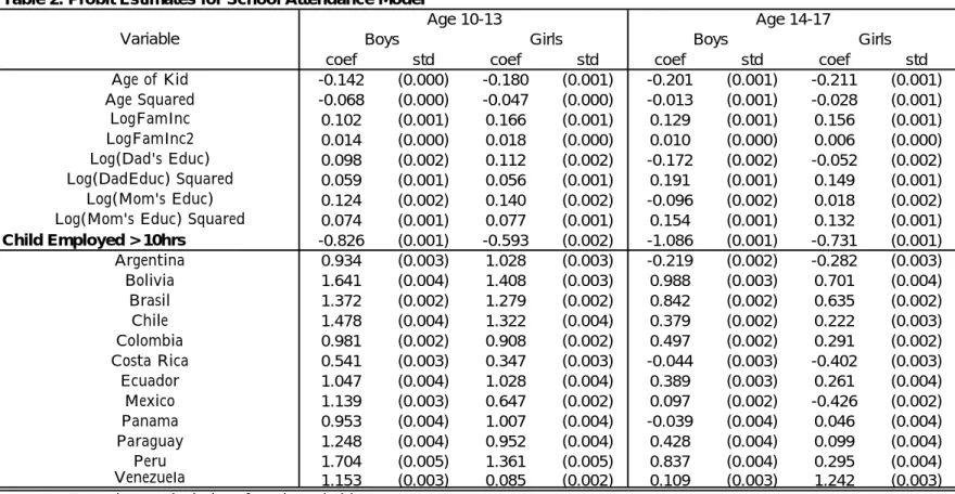
A key assumption in the paper is that child labor reduces education. Some empirical evidence for this assumption is presented in Table 2. The table shows results for a probit regression in which the dependent variable is an indicator equal to one for kids in school, and zero otherwise. The explanatory variables include an employment variable, the age of the child and family characteristics, such as household income, father’s education and number of kids aged less than 6 years old. The employment variable is set to 1 if kids worked 10 hours per week or more, zero otherwise. Age variables are based on deviations from the mean, while income variables appear as deviations from the median; both appear in the regression equation as the logs and the squares of the logs. Consider a family in which the parents have 6 years of education each, and earn the median income. Suppose they live in a country where thefixed effect = 1. The table suggests that employment reduces the probability that
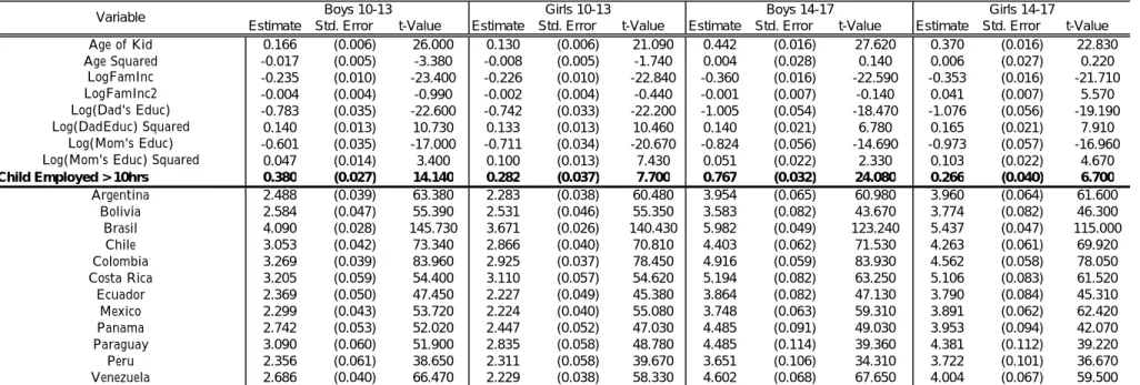
a child aged 10-13 attends school from 91% to 75% for boys and from 93% to 86% for girls. An alternative measure of the impact of child labor on education is the education gap, which equals the potential education of the child as a function of age, less the attained education, measured in years. Table 3 shows OLS estimation results for a regression of education gap on the same explanatory variables described above. The estimates suggest that employment increases the gap by 0.38 years for boys in the younger group, and by 2.82 for girls. For the older group, the estimates are 0.767 and 0.266, respectively. These numbers are associated with high t-values, and reinforce the impression from the previous table, that child labor competes with education in the allocation of children’s time. While these numbers do not seem large as a percent of average educational attainment, it is likely that children with interrupted schooling will not return; hence a positive gap indicates that attainment will not increase with age. This argument is explored explicitly in Psacharapoulos (1981), who reports even larger education gaps associated with child employment in Peru.
Obviously there is no attempt here to deal with unobserved heterogeneity or with co-linearity among the explanatory variables. If less able students were more likely to leave school , then these estimates would represent upper limits on the effect of child labor. On the other hand, assuming that parental income does not directly affect education, the bias resulting from co-linearity between employment and family income is clearly towards under-stating our result: children with low income do worse in school, holding ability constant, because they are more likely to be employed. In the absence of further evidence, it is rea-sonable to assume that the results are not driven by bias from omitted variables, and hence we conclude that child labor does indeed have a large and significant effect on educational attainment.
2.3. Country Effects on Child Employment
To see how child-labor patterns vary across countries, we report in Table 4 results for a regression of child labor-hours on parental income, parental education and the age of the child, as well as a set of dummy variables for each country. The table shows that children’s
hours are higher among the older age group of children, and that the cross-country patterns are otherwise similar across age groups. Parental income reduces the probability of child employment, as does education of the parents, with mother’s education having a slightly larger effect than father’s education. Hence the impression that emerges is that child labor is a response to poverty, and parents use higher income to purchase more time in education for their child.
The main message of the countryfixed-effects in the table is that child labor participation depends on the country of origin, even after controlling for parental income. The unexplained component of children’s hours is significantly higher in Bolivia, Brasil, Paraguay and Peru than in the other countries. Therefore child labor is not merely a matter of parental poverty: there is a significant social effect as well. It turns out that Bolivia, Peru and Paraguay are the poorest countries in the sample, on a per-capita basis, while Brasil has the most unequal distribution of income8. Hence it is likely that the common denominator across countries with high child labor is indeed a low median income. Countries where child labor is least likely, controlling for parental income are Argentina, Panama and Chile; hence the fact that two of these are the most prosperous countries in the sample supports the idea that there is an income-based explanation of the country-effects on child labor.
2.4. Explaining the Country Effects
We interpret thefixed effects estimated in Table 4 as indicators of the permissiveness of the countries in question towards child labor. In this section we examine how these effects are correlated with per capita income and with whether a country has ratified the ILO’s C-138 convention against child labor.
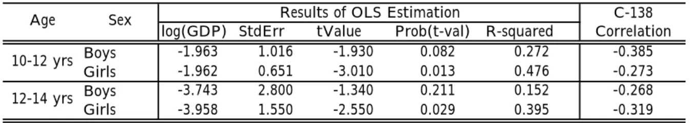
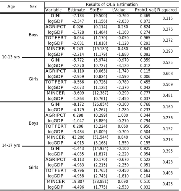
Table 5 shows how these estimated fixed effects relate to per capita GDP. The relation between GDP and the child labor fixed effect is negative, and often quite strongly so; the estimated coefficient is shown in the row labeled “log(GDP)”, and below it the standard 8See Facing up to Inequality in Latin America, 1998, Inter-American Development Bank, Washington,
error, the t-statistic, the probability of the t-statistic under the null hypothesis, and the R-squared coefficient. 9 The country-GDP relation is much stronger for girls in both age groups than for boys; labor supply of girls declines more quickly with per capita GDP. It is significant that in all cases, the relationship is stronger for the younger age group than for the older, which is consistent with our interpretation, as we would expect more restrictions on child labor for the younger age group. This strong relation between GDP and the country effects suggests that an increase in GDP reduces child labor not only via higher family income of high-risk families, but also via some aggregate effect.
It is encouraging therefore to note the consistently negative correlation between these effects on the one hand, and a country’s support of convention C-138 on the other. Data on whether a country is one of the 89 countries that have ratified this convention, which dates to 1973, is available from the ILO web site. The convention states that “National policy must aim to ‘ensure the effective abolition of child labor’...”. 10 The consistent negative sign of these correlations, reported in thefinal two rows of Table 5, suggests that countries which we find more open to child labor are less likely to have officially endorsed the convention against child labor, which is what one would expect if our indices are in fact reflecting the hostility of the general legal and political climate of a country towards child labor.
Robustness is of course a major issue in this type of regression analysis, particularly with so few data points. An important possibility is that the explanatory variable is actually reflecting the effect of some other variables with which it is correlated. These indicators of child labor are essentially residuals, and hence do not distinguish between the effects of child labor laws and other factors omitted from the regression that may also influence child labor. This issue is addressed in Table A3, which shows the effect of including a second aggregate variable in the regression of the country effects on GDP per capita. The variables, whose 9Quadratic terms had very little effect on R-squared, so these higher-order regressions are not reported. 10According to the ILO web site, www.ilo.org/public/english/standards/norm/whatare/cld_paper.htm
“The States that ratify this convention must, inter alia, protect the child from economic exploitation and from performing any work that is likely to interfere with his education, or be harmful to his health or well-being.”
values are given in Table A2, are the Gini coefficient for income, the total fertility rate, the percent of the country’s GDP accounted for by agriculture, and the rate of return to education. This last variable, the Mincer coefficient, is taken from Bils and Klenow (2000). The result is that GDP remains statistically significant for girls, while for boys the GDP effect is no longer statistically significant when other variables are added to the regression. This is to be expected due to the small size of the sample. However what is interesting is that the sign of the GDP effect remains negative in all cases. Furthermore, in the most successful models, such as the girls 10-13, particularly the specification with agriculture, the GDP coefficient is more significant than in the single-variable regression, and R-squared much higher.
In conclusion, it appears that GDP per capita does inhibit child labor, even after taking into account household income. The sample is too small to allow multi-variate analysis, but thefinding appears robust to inclusion of other variables. The estimated country effects behave as one might expect for an indicator of child labor permissiveness: they are negatively correlated with ratification of the ILO’s anti-child labor convention, and they are stronger for young children than for older.
3. A Model of Child Labor
The empirical analysis above suggests that there is considerable variation within Latin Amer-ica in regards to the tendency of children to work, and it is likely that this reflects variations in the legal status of child labor across countries. In this section we present a simple theory of parental decisions regarding the allocation of children’s time between labor and education. Under our assumptions, parents may favor child-education laws because they help parents to commit to more education for the child. The key assumptions are: 1) child labor reduces education, 2) parents get utility from the education of their children, 3) parental preferences are time-inconsistent, and 4) the median voter is decisive. The main result of the model is that parents optimally choose laws that restrict children to a minimum time spent in school. Consider an economy where agents live for 2T + 1 periods, the first T as children, and
thenT+1periods as parents, with one child born when the parent is agedT. The parent has an endowment of human capital hp and receives labor income whp. Children may become workers from the time that the parent is aged T + 1. Their human capital on attaining adulthood at period T is given by hc
T, which depends on the fraction ect of their time they have allocated to their education at each age. This allocation is decided by the parent. The child’s initial human capital is hc
0, and evolves deterministically according to the function:
hct+1 =φ(h c t, e c t) (3.1) .
Parents get utilityu(cτ) from their own consumption in each periodτ of their ownfinite
lives and utility ν(hc
T) in the final period of life from the final level hcT of their children’s education. Parent’s discount factors for future utility are quasi-geometric; the discount factor between adjacent future periods is β ∈ (0,1), but between the present and the immediate future, the discount factor isβδ∈(0,β). Preferences take the following time-separable form:
U0 =u(c0) +δ " βTν(hcT) + T X τ=1 βτu(cτ) #
We interpret delta as a measure of the severity of the time-inconsistency problem: as we will see below, the lower is delta, the greater is the range of parental income over which the parent’s inability to commit leads to a lower level of the child’s education.
Children’s labor income depends on the fraction of time(1−ec
t)the child works in period t, and on the child’s effective wagewc
t, which is the basic child’s wagewc1, times the child’s
productivity premium for age. The child’s wage is not a function of the child’s human capital.11 Furthermore, following Cain (1977), it is assumed that a child aged t+ 1 is the productive equivalent of (1 +γt) children aged t. Therefore a child aged t+ 1 will face an effective wage rate
wct+1 = (1 +γt)wct, 0≤γt<1
11This assumption is standard in the literature on child labor; see Glomm (1997); Baland and Robinson
allt. As the child grows older, the productivity premium for age,γt,declines, as the child’s wage converges toward the adult wage. A direct implication is that the sequence of age-specific productivity differentials {γt}
T
t=1 converges from above towards zero ast approaches
T.
In each period t ≤T, parental consumption is constrained by the total household labor income, which is equal to the sum of parental labor income and that of the child. Let pt denotes the period-t per unit education cost reflecting for example, expenditures on school supplies, registration fees, transportation costs etc. Then the parent period-t budget con-straint is given by:
ct≤wphp+ (1−ect)wct−ptet (3.2) This parental budget constraint implies that, in addition to the direct cost, ptet, of educating a child, there is also an indirect cost, in the form of household income foregone from child labor sourceswc
tect.The essential point, that child labor significantly reduces both educational time and eventual attainment, is well supported by empirical studies, such as Rosenzweig and Evenson (1977) and Psacharopoulos (1997).
In theirfirst period, children are physically incapable of working, so parental consumption equals wphp. Since parents make no time-allocation decisions this period, when their child has age t= 1, it will be ignored below, except to consider voting over labor laws.
It will be assumed below that the above functions obey the following standard conditions:
U.1 u0 >0;u00 <0; u0(c)→ ∞ as c→0;u0(c)→0as c→ ∞.
U.2 v0 >0; v00<0;v0(h)→ ∞ ash→0; v0(h)→0 ash→ ∞.
U.3 φe >0,φh >0,φee <0,φhh<0,φe,h>0.
Assumption 3 implies that education time and previous attainment are complements in the production of next period’s attainment. Furthermore the second-derivative assumptions imply enough concavity that interior solutions, when they exist, are optimal.
3.1. Optimal Education Decisions
In general the choice of education at time T −j will deviate for two reasons from the choice of a parent who can commit att= 0. First is the direct effect of impatience, i.e. the change in discount factor between T −j andT −j+ 1. Second, there may be strategic interaction between the parent’s decisions at different time periods. These effects are illustrated below. It is straight-forward to solve the parent’s problem by backwards induction. In the last period of life, the parent’s payoff is given by ν³φ³hc
T−1, ecT−1 ´´
. Therefore when allocating the child’s time between education and labor in the penultimate period, the parent faces the following dynamic programming problem:
VT0−1 ³ hcT−1, hp ´ = max ec T−1 n uhwphp+³1−ecT−1 ´ wcT−1−e c T−1pT−1 i +βδν³φ³hcT−1, e c T−1 ´´o , subject to (3.2) and (3.1).
An interior solution satisfies the following first-order condition:
h wcT−1+pT−1 i u0(cT−1) =βδν0(hcT)φe ³ hcT−1, ecT−1´ (3.3) . Diminishing marginal utility implies that if the optimal ecT−1 is interior, then the child’s
education will be increasing in the parent’s human capital,h0. Furthermore, the presence of
δ on the right hand side implies that the education choice, if interior, will be strictly less than what the parent would have chosen could he have committed to ec
T−1 at some earlier
time.
Given the above assumptions, it is important to ask whether parents whose children have higher level of human capital carried over from the preceding period will tend to invest less in their children at time T −1. As shown in the following proposition, the answer to this question depends upon whether a marginal increase in the level of human capital carried over from the previous periods “sufficiently” raises the marginal productivity of child’s time allocated to education:
Proposition 1. Let assumptions U.1−U.3 hold. Then (i), if
φeh < −ν
00
∂eT−1/∂hcT−1 <0. Furthermore, (ii) ∂eT−1/∂hp >0, and (iii) ∂eT−1/∂δ >0, where eT−1 =
gT−1(δ, hp, hcT−1) denotes the interior solution to (3.3).
P roof. Given the properties of the functions u,ν, andφ, the second order condition for a maximum is satisfied: hwc
T−1+pT−1 i2
u00+βδhν00φ2
e+ν0φee
i
< 0. The implicit function theorem may then be applied to establish all three results.
Condition (3.4) states that the increase in the productivity of time allocated to schooling due to a marginal increase in the level of human capital carried over from the previous periods is not “too” large. Part (i) of proposition 1 states that child’s time allocated to education tends to be smaller(greater), the higher (smaller) the child’s human capital level carried over from the previous period. Part (ii) of proposition 1 states that richer parents tend to invest more on their children’s education. Part (iii) states that child’s time allocated to schooling declines with the severity of the time-inconsistency problem.
To define the solutions for the preceding periods, it is convenient to analyze the parental decision as the outcome of a 2-stage dynamic-programming problem, as in Laibson, Repetto, and Tobacman (1998) and Krusell and Smith (1999). Using the definition of the optimal education policy, the resulting children’s human capital is given by:
hct+1 =φ[hct, gt(δ, hp, hct)]. (3.5) At time T −2, the parental problem is to maximize:
VT0−2 ³ hcT−2, hp ´ = max ec T−2 n uhwphp+³1−ecT−2 ´ wTc−2 −ecT−2pT−2 i +βδWT0−1 ³ hcT−1, hp ´o subject to WT0−1³hcT−1, hp´ = uhwphp+³1−g³hTc−1;hp´´wcT−1−g³hcT−1;hp´pT−1 i (3.6) +βhν³φhhcT−1, g³hcT−1;hp´i´i andhc T−1 =φ h hc T−2, ecT−2 i
, where(3.6) denotes the continuation value at T −1.
From the point of view of periodT −2, the discount factor between periodsT −1andT is given by β, but the parent knows that when the time comes to chooseec
T−1, the discount
The first-order condition at time T −2is: −hwTc−2+pT−2 i u0(cT−2) +βδ ∂W0 T−1 ³ hc T−1, hp ´ ∂hc T−1 φe ³ h1T−2, e c T−2 ´ = 0. (3.7) This first order condition is satisfied by the education timee that equates the marginal cost of educating the child atT−2to the marginal (future) utility from raising the child’s human capital level. Given that the parent will act impatiently in the future, atT−2 she perceives the marginal benefit of education as:
∂WT0−1 ³ hcT−1, hp ´ ∂hc T−1 = ∂gT−1 ∂hc T−1 ·h−hwTc−1+pT−1 i u0(cT−1) +βν0 ³ h1T´φec ³ hcT−1, gT−1 ´i +βν0³h1T ´ φh ³ hcT−1, gT−1 ´ (3.8) where gT−1 ≡gT−1(δ, hcT−1, hp).
The second term on the right hand side is perfectly standard; thefirst term however only appears due to the time-inconsistency of the parental preferences; otherwise the envelope theorem tells us that the term multiplying the policy function derivative would be zero at the optimum, in which case
∂W0 T−1 ³ hc T−1, hp ´ ∂hc T−1 =βν0³h1T´φh ³ hcT−1, gT−1 ´
. However without commitment, it becomes important to investigate whether the marginal benefit of an additional increment in the child’s level of human capital carried over from the preceding period (the term∂W0
T−1 ³ hc T−1, hp ´ /∂hc
T−1) turns out to be larger or smaller than
the level that would obtain under commitment ( the term βν0(h1T)φh
³
hcT−1, gT−1 ´
). The answer to this question is summarized by the following proposition.
Proposition 2. Let condition (3.4) hold. Then
∂WT0−2 ³ hcT−1, hp ´ ∂hc T−1 <βν0³h1T´φh³hcT−1, gT−1 ´ .
P roof. Since condition (3.4) hold, by proposition 1, ∂gT−1/∂hcT−1 < 0. Furthermore,
since by proposition 1∂gT−1/∂δ >0, then
−hwTc−1+pT−1 i u0hwphp+ (1−gT−1)wTc−1−gT−1pT−1 i +βν0³h1T ´ φec ³ hcT−1, gT−1 ´ >0,
implying that the policy gT−1(δ, hcT−1, hp) is sub-optimal from the point of view of period
T −2. Hence the result.
Proposition 2 states that both the direct and strategic effects of time inconsistency reduce the perceived future benefits of educating the child atT −2. This in turn causes parents to choose inefficient levels of child’s schooling time in each period.
Earlier stages of the game are solved by applying the same approach. At time T −3, the parental problem is to maximize:
VT0−3³hcT−3, hp´= max ec T−2 n uhwphp+wcT−3−eTc−3³wcT−3+pT−3 ´i +βδWT0−2³hcT−2, hp´o subject to the continuation value from the period T −3point of view,
WT0−2³hcT−2, hp´ = uhwphp+wcT−2−ecT−2³wTc−2 +pT−2 ´i (3.9) +βWT0−1³hcT−1, hp´ the policy ec T−2 =g ³ hc T−2;hp ´
, the continuation value from the period T −2point of view, WT0−1 ³ hcT−1, hp ´ =uhwphp +wcT−1− ³ wTc−1+pT−1 ´ g³hcT−1;hp ´i +βν³φhhcT−1, g ³ hcT−1;hp ´i´ andhc T−1 =φ h hT−2, g ³ hc T−2;hp ´i . Consider ∂WT0−2 ³ hcT−2, hp ´
/∂hcT−2. It can easily be established that
∂W0 T−2 ³ hc T−2, hp ´ ∂hc T−2 = ∂gT−2 ∂hc T−2 · −hwcT−2+pT−2 i u0(cT−2) +β ∂W0 T−2 ³ hc T−2, hp ´ ∂hc T−2 φe³hcT−2, gT−2 ´ +β∂gT−1 ∂hc T−1 ·h−hwcT−1+pT−1 i u0(cT−1) +βν0 ³ h1T´φe³hcT−1, gT−1 ´i φh³hcT−2, gT−2 ´ +β2φh³hcT−2, gT−2 ´ ν0³h1T´φh³hcT−1, gT−1 ´
Note that the first two terms are negative due to strategic interaction. Therefore adding more periods worsen the effect of time -inconsistency in the sense that the future benefits of educating the child today becomes even smaller.
To solve for the complete sequence of education investments is simply a matter of con-tinuing the procedure of backwards induction described here all the way back to the first period of the child’s life. If the conditions of proposition 2 are satisfied, this means that adding more periods to the analysis will further aggravate the time-inconsistency problem but not qualitatively change our results, so from now on we restrict attention to the simple caseT = 3.
3.2. Parametric Example
In this section we sacrifice some of the richness of the model in order to obtain analytical results. We consider a simple 2-period version of the model with logarithmic preferences and Cobb-Douglas technology. This specification implies the strategic effect is zero. What do we lose by restricting the model in this way? Under the conditions of Proposition 2 above, the strategic interaction effect and the addition of more periods of education both intensify the time-inconsistency problem, so in a world characterized by these conditions, the simple version below could be considered a reduced-form version of the full model, in which the time-inconsistency parameter δ is made smaller to reflect the two omitted effects.
For the policy analysis to be conducted here, we need the answer to two questions: (1) Who benefits from banning child labor? and (2) How does the optimal level of compulsory education depend on the parental state? Some analytical results are possible for a sufficiently simple choice of time structure and functional forms. Since the data we have on children’s education and labor time is available only for two periods (primary and secondary education), we restrict the analysis to education decisions over two periods of childhood.
Suppose that T = 3, so that parents choose their children’s activities for two periods. Let u(c) = lnc and ν(h1
T) = Alnh1T, where A > 0. Human capital in every state is now given by: hct =φ ³ hct−1, ect−1 ´ = hc1 t = 1 ³ hc t−1 ´η³ e+ec t−1 ´1−η t > 1 where η>0.
Notice that as long as e > 0, the functional form for the human capital accumulation technology allows for children to have positive human capital even in the absence of parental investment in schooling. We show in appendixA.1that with respect to their optimal choice of education policy pairs, (e∗
1, e∗2), parents can be classified in four groups determined by
their human capital levels. In particular, under certain conditions, all parents with human capital levels in the range:
(i) [h, H1(δ)] choose (e∗1, e∗2) = (0,0) (ii) ³H1(δ),H¯1(δ) ´ choose (e∗ 1, e∗2) = (ec1,0) (iii) ³H¯1(δ),H¯2(δ) ´ choose (e∗ 1, e∗2) = (1, ec2) (iv) hH¯2(δ),h¯ i choose (e∗ 1, e∗2) = (1,1) where ec1 = d1 1 +d1 · w(hp, p1, wc1)− e d1 ¸ ec2 = d2 1 +d2 ³ w(hp, p2, wc2)−d− 1 2 e ´
and h ≤ H1(δ) < H¯1(δ) < H¯2(δ) ≤ ¯h. Note the dependence of the size of the respective
ranges on the time-inconsistency parameter, δ. This implies that the distribution of the population of parents across these ranges is affected by the degree of severity of the time-inconsistency problem. Hence the following proposition:
Proposition 3. The lower is δ, (i) the larger the number of parents who choose not to educate their children in all periods ( i.e., parents who choose (e∗
1, e∗2) = (0,0); and (ii) the smaller the number of parents who choose to educate their children full-time in all periods ( i.e., parents who choose (e∗1, e∗2) = (1,1)).
P roof. It suffices to note that H1(δ) (respectively H¯2(δ)) is higher the smaller δ (i.e.,
Proposition 3 is the parametric analog of proposition 2; it establishes the potential
inef-ficiency of parental education policies due to the time-inconsistency problem. Note however that sinceH1(δ)(respectivelyH¯2(δ)) is smaller the higherδ, andδ ∈[0,1], for parents whose
human capital levels fall within the range [h, H1(1)] or h
¯ H2(1),¯h
i
, time-inconsistency is not a problem. Parents with human capital in the interval [h, H1(1)] are just too poor to afford
to give up on income from child labor sources, hence (e∗
1, e∗2) = (0,0). In contrast, parents
with human capital in the intervalhH¯2(1),h¯ i
are rich enough to pass on the opportunity to supplement household income with income from child labor sources, hence (e∗
1, e∗2) = (1,1).
While for the first group of parents, –the poorest ones– banning child labor will result in a welfare loss, for the second group, –the richest parents–there will be no welfare change. This raises the issue of whether there are parents who can be made better offby such a ban. We address this issue below.
4. A Reduction in Children’s Wages
An important policy issue in many prosperous countries today is whether to restrict imports of goods made using child labor. The professed objective of such policies would be to make the children better offby preventing their exploitation as workers, and lower the opportunity cost of their education. Under standard preferences, an exogenous change in the children’s wage reduces the welfare of those parents whose children were working before the change. In our model, it is possible that some parents are made better off by such a change. In this section we explore conditions required for this to happen. We show that while some families may indeed be better off, in an ex ante sense, as a result of such a policy, these families are not necessarily the poorest ones.
From the point of view of a poor household considering how to allocate children’s time, the effect of such a policy would be perceived as a reduction in the wage for child labor. For parents to gain from a reduction in the child’s wage, there must be in increase in their
indirect utility from the view point of period T −2. This is given by WT0−2³hcT−2, hp, w1c, p1, p2 ´ = uhwphp+wc1−g1 ³ hcT−2, hp, wc1, p1, p2 ´ (wc1+p1) i +βWT0−1 ³ hcT−1, hp, wp, wc1, p2 ´ where WT0−1 ³ hcT−1, hp, wp, w c 1, p2 ´ = uhwphp+ (1 +γ)wc1−g2 ³ hcT−1, hp, w c 1, p2 ´ [(1 +γ)w1c+p2] i +βν³φhhcT−1, g2 ³ hcT−1, hp, w c 1, p2 ´i´
since we restrictT to equal 3.
Now consider the effect, on parents’ welfare, of an exogenous change in the basic child labor change, wc. Denote this effect as∂W0
T−2 ³ hc T−2, hp, wc1, p1, p2 ´ /∂wc 1. In appendix A.2
we prove the following result.
Proposition 4. Suppose that utility satisfies constant elasticity of substitution and parental education policies are in the interior of the choice set. Then there exists a threshold e
h(δ)such that if hp > he(δ), then
∂ ∂wcW 0 T−2 ³ hcT−2, hp, w c 1, p1, p2 ´ <0.
Furthermore, the more severe the time-inconsistency problem, the wider the range of parental human capital such that all parent with human capital within this range can be made better off by an exogenous reduction in the child labor wage.
P roof. See appendix A.2
This says that some parents may indeed gain from a reduction in the children’s wage, but that in general there may be poorer parents who will lose. Thus our model supports the idea that sanctions on child labor may make some poor families better off, but with the risk of hurting even poorer families, as argued above. In all cases of course, children’s education will increase, but this is partly due to the simplifying assumption of no direct costs of children’s education, such as tuition fees or nutrition.
It is important to note that this result does not rely on the assumption of direct costs of education, such as tuition fees or materials; these have been included to demonstrate
the robustness of our basic model. Obviously,such costs reduce the set of winners for two reasons. First, by raising the cost of education, the gains to making children attend school are reduced. Second, the wage-reduction policy, by lowering the revenue of those families whose children acquire a partial education, will reduce the education of these children even further. However in many countries, education, at the primary level at least, is heavily subsidized, so our analysis can be simplified by omitting direct costs.
5. Compulsory Education
We now explore the conditions required for the emergence of compulsory-education laws. The key assumption we make here is that laws are chosen by the median voter in an election in which the only issue is how high to set the minimum amount of time children should spend in school.12 We also assume that parents who would choose full-time education for their own children, and therefore do not directly benefit from mandatory-education laws, will also support laws requiring full-time education.
There are 3 cases, one where the minimum binds in both periods, the others where it binds in one only. The latter cases are less interesting because they are equivalent to the median voter making the optimal education choice ex ante. In this section, only the first case is considered. To focus exclusively on the determinants of the timing of the adoption of laws restricting child labor, we set γ = 0. Therefore, where the minimum schooling binds in both periods, the median voter chooses ebto solve:
max be ½ (1 +β) ln [wphp+wc(1−e)] +b β2Aln·³h11 ´η2 (e+e)b (1+η)(1−η) ¸¾
Note the absence of the time-inconsistency parameter, δ, on the median voter’s problem. This is because voting acts as a commitment mechanism, in which case δ= 1.
Proposition 5. The minimum level of compulsory education is an increasing function
12To ensure that richer countries would ban child labor altogether, we would also need to assume that
parents who are suffficiently rich so as to choose zero labor for their children will either favor compulsory schooling or abstain from voting on education laws.
of the median voter’s income. Furthermore, unless the median voter’s income is above a threshold H(wpf , wc), there will be no political support for compulsory education, where
f H(wp, wc) = [(1 +β)e−C0] Ã wc wp ! . (5.1)
P roof. The first-order condition to the above problem is: (1 +β)wc wphp+wc(1−e)b =β 2 A e+eb(1 +η) (1−η) = C0 e+eb
where C0 ≡Aβ2(1 +η) (1−η). The preferred choice of education law is given by: b
e= (1 +β+C0)−1[C0we(hp)−(1 +β)e] (5.2)
. That the level of compulsory education rises in the median voter’s income simply follows from the fact that ∂ˆe/∂hp >0. The threshold H(wp, wc)f is simply solution to the equation ˆ
e= 0.
Notice that the choice of eˆis independent, for the reasons discussed earlier, of the time-inconsistency parameter δ. Empirically, the implication of ∂e/ˆ ∂hp > 0 is quite direct: if countries all share the same parameter values, then compulsory education should be a linear function of the wage ratio of the median voter. This behavior should hold over the range for which human capital makes a difference for education laws. Countries with child-labor restrictions will be those for whiche >b 0. From (3.1), this implies a condition on the median voter: hp >[(1 +β)e−C0] Ã wc wp ! .
For countries where the value of the median voter’s human capital falls below this thresh-old, increasing median income will reduce child-labor only via household income; above this threshold, there will be an additional effect of income on child labor, via the laws governing compulsory education. Thus the theory fits with the basic empirical observation we made earlier that the unexplained variation in children’s labor across countries is negatively cor-related with the GDP of the country, provided that median and average GDP are strongly correlated.
A basic empirical test could be performed, if data on children’s wages were available, by regressing the measures of child labor discussed in the empirical section of this paper on median income and the ratio of children’s wages to those of unskilled adults. Such a test would raise two issues: equilibrium wage determination and parametric differences across countries. If the demand for child labor were sufficiently inelastic, then countries with high equilibrium wage ratios could be those where child labor is less prevalent. Since child labor is relatively unskilled by assumption, such conditions are unlikely. Parametric variations are more likely to be an issue. Variations across country in the quality of available education, for instance, affects the parental decision via the return to education, here represented by the parameterη, which is the share of school time in the human capital of the child.Another important dimension along which countries may vary is the degree to which elderly parents receive utility from their children’s education. The wage-skill premium would be one source of such variation, but perhaps equally important is variation in the dependence of parents on support from children in old age. Thus our theory of child labor laws is empirically verifiable, but we leave this for future research.
6. Conclusion
This paper asked how laws against child labor might emerge despite the lack of motivation for such laws in standard household decision theory. Our motivation for asking this question is that while standard theory does not seem to explain why households would vote for such laws, these laws are often credited with a significant role in reducing child labor, as in Doepke (1999) and Moehling (1999). We presented an empirical analysis of child labor in Latin America that supports the hypothesis that the country of residence has an effect on the propensity of children to work, and showed that this effect is more strongly negative in countries with higher levels of per capita income. The data suggest that these country effects are not explained by cross-country variations in the return to education, not by other plausible candidates, such as the share of agriculture in GDP or the fraction of the population living in urban areas.
Although the empirical analysis was limited by the small number of countries in the dataset used here, ourfindings were robust to the inclusion of other variables. We interpreted this country effect on child labor as consistent with the effects of variations in child labor laws, noting a small but consistent correlation between our measure of the country effect and whether the country had officially endorsed the ILO’s conventions C-138 against child labor.
We then presented a theory of child-labor based on the assumption that parents have time-inconsistent preferences and showed how, in the absence of other institutions allowing parents to commit, child-labor laws may increase the welfare of poor households in an ex ante sense by allowing parents to achieve a higher level of education for their children than they would be able to achieve with an unconstrained choice set. Our model does not require parents somehow to be able to commit to laws; a lag between the vote and the enforcement of the laws is all that is required. We showed that child labor laws emerge when the median voter has income in an intermediate interval that depends on the returns to the parent of the child’s education. While the median voter is in this range, an increase in per-capita income will reduce child-labor supply of a given household, even after controlling for household income.
Another theoretical implication of the model is that measures that reduce the wage of children, such as a ban by foreigners on the import of goods made by child labor, will reduce the welfare of households who are sufficiently poor, but raise that of households that are somewhat richer. Thus a restriction on child-produced imports by wealthy countries, a policy that is often motivated as a way to help child workers, may indeed have the desired effect, but at the expense of children who were even worse off. Thus to assess such a policy it is necessary to know how the distribution of poor households is divided between these two categories.
From the point of view of assessing the long—run benefits of policies restricting child labor, an obvious next step for the model developed here would be nesting it into a dynamic model of the income distribution, such as that of Galor and Zeira (1993). Analysis along such
macroeconomic lines would allow us to relate the issues raised here to long term deveopment, as in Doepke (1999), who incorporates fertility decisions into a growth model where parents choose whether to educate their children. Thus we can see the current paper as a building block towards assessing the effects of policies to reduce child labor in developing countries.
References
Anker,andMelkas (1996): “Economic Incentives for Children and Families to Eliminate or Reduce Child Labor,” ILO Documentation.
Basu, K. (1999): “The Intriguing Relation between Adult Minimum Wage and Child La-bor,” Policy Research Working Paper 2173.
Basu, K., and P. Van (1998): “The Economics of Child Labor,” American Economic Review, 88 (3), 412—27.
Becker, G. S.(1976): The Economic Approach to Human Behavior. University of Chicago Press, Chicago, IL and London,UK.
Becker, G. S., K. M. Murphy, andR. Tamura (1990): “Human Capital, Fertility and Economic Growth,”Journal of Political Economy, 98(5, pt. 2).
Bils, M., and P. J. Klenow (2000): “Does Schooling Cause Growth?,” American Eco-nomic Review, 90 (5), 1160—83.
Cain, M. (1977): “The Economic Activities of Children in a Village in Bangladesh,” Pop-ulation and Development Review, pp. 201—227.
Dahan, M., and A. Gaviria(1999): “Sibling Correlations and Intergenerational Mobility in Latin America,” Mimeo,IDB.
Dessy, S. (2000): “A Defense of Compulsory Measures against Child Labor,” Journal of Development Economics, Forthcoming.
Doepke, M.(1999): “Growth and Fertility in the Long Run,” Mimeo,University of Chicago.
Fang, H., and D. Silverman (2000): “Dole Meets Laibson: On the Compassion of Time-limited Welfare,” Mimeo,University of Pennsylvania.
Galor, O., and J. Zeira (1993): “Income Distribution and Macroeconomics,” Review of Economic Studies, 60(1), 35—52.
Glomm, G. (1997): “Parental Investment in Human Capital,” Journal of Development Economics, 53 (3), 99—114.
Goldin, C. (1979): “Household and Market Production of Families in a Late-Nineteenth Century American Town,”Explorations in Economic History, 16(2), 111—31.
Grootaert, C., and R. Kanbur (1995): “Child Labor: An Economic Perspective,”
International Labor Review, 134(2), 187—203.
Krusell, P., and T. Smith (1999): “Consumption and Savings Decisions with Quasi-Geometric Discounting,” Mimeo,University of Rochester.
Laibson, D. (1997): “Golden Eggs and Hyperbolic Discounting,” Quarterly Journal of Economics, 0, 443—477.
Laibson, D., A. Repetto, and J. Tobacman (1998): “Dynamic Choices of Hyperbolic Consumers,” Mimeo, Harvard University.
Moe, K. S. (1998): “Fertility, Time Use and Economic Development,”Journal of Political Economy, 1, 699—718.
Moehling, C. M. (1999): “State Child Labor Laws and the Decline of Child Labor,”
Explorations in Economic History, 36(72), 72—106.
Psacharapoulos, G. (1981): “Returns to Education; an Updated International Compar-ison,”Comparative Education, 17, 321—341.
Psacharopoulos, G. (1997): “Child Labor Versus Educational Attainment: Some Evi-dence from Latin America,”Journal of Population Economics, 10, 377—386.
Rosenzweig, M., and R. Evenson (1977): “Fertility, Schooling and the Economic Con-tribution of Children in Rural india,”Econometrica, pp. 1065—1079.
Szekely, M., and M. Hilgert (1999): “What’s Behind the Inequality We Measure: An Investigation Using Latin American Data for the 1990’s,” Mimeo, Inter-American Devel-opment Bank.
Appendix A.1
In this appendix, we solve for the parental education policies e1 and e2. Once again,
the analysis proceeds by backwards induction from the final period. In the last period, the parent simply enjoys his child’s human capital, so thatV0
3 =ν(hc3). Terminal human capital
hc3 is given by:
hc3 = (hc2)η(e+g2(hc2;hp)) 1−η
The following technical assumption will prove necessary to derive the analytical results.
U.4 e > Aβ(1−η).
Suppose that the parent chooses in each period the time spent in education. The parental problem in the 2nd period is:
V (hc2, hp) = max ec 2 U(hc2, hp, ec2) where U(hc2, hp, ec2) = ln [wphp+ (1−ec2)w2c−p2e2] +βδAln h (hc2)η(e+ec2)1−ηi (.1) . The first-order conditions for an interior solution is:
ec2 : −(w c 2+p2) wphp+ (1−ec 2)w2c−p2e2 + βδA(1−η) e+ec 2 = 0 (.2) . Lettingd2 ≡βδA(1−η), it can be shown that the optimal education policies are:
ec2∗ = 0 if hp ≤H2(δ) d2 1+d2 ³ w(hp, p2, w2c)−d− 1 2 e ´ if H2(δ)< hp <H¯2(δ) 1 if hp ≥H¯2(δ) (.3) where w(hp, p2, wc2) = wphp+wc 2 p2 +wc2
H2(δ) = " e d2 Ã 1 + p2 wc 2 ! −1 # wc 2 wp ¯ H2(δ) = " (1 +d2+e) d2 Ã 1 + p2 wc 2 ! −1 # wc 2 wp
Note that since by assumption U.4, e. > Aβ(1−η) and δ ∈ (0,1), it is guaranteed that H2(α,δ) andH¯2(α,δ) are strictly positive.
For any program and any state, we can define the value of the program from the point of view of the first period as:
W2(ec2, h c 2, hp) =u(e c 2|hp) +βν[φ(e c 2|h c 2)] (.4)
The value, from the point of view of the first period, of entering the second period with state (hc
2) is given by the value of W2, evaluated at the program chosen by the 2nd-period
agent. In particular, evaluating (.4) at the optimum yields W∗
2 (hc2, hp) = W2(ec2∗, hc2, hp) where W2(ec2∗, h c 2, hp) = ln [wphp+w c 2−(w c 2+p2)ec2∗] +βAln h (h2c)η(e+e2c∗)1−ηi (.5) where ec2∗ ≡g2(hc2, hp).
Now consider the effect on the continuation value,W2(ec2∗, hc2, hp), of a marginal change
in hc2, and denote this effect as ∂W2(e2c∗, hc2, hp)/∂hc2. Using (.5) this expression reduces to:
∂W∗ 2 (hc2, hp) ∂hc 2 = " −[wc 2+p2] wphp+wc 2−(wc2+p2)ec2∗ +βA(1−η) e+ec∗ 2 # ∂ec∗ 2 ∂hc 2 + βAη hc 2 , (.6)
whereW2∗(hc2, hp) =W2∗(ec2∗, hc2, hp). Since the second period education policy is independent
of hc
2, therefore ∂ec2∗/∂hc2 = 0, implying that
∂W∗ 2 (hc2, hp) ∂hc 2 = βAη hc 2 (.7) The above remarks will prove useful for solving the first-period problem.
Each period-one parent chooses the education investment program given the program chosen by the 2nd-period parent. We can write this as:
V (hc1, hp) = maxec 1 { ln [(wphp+ (1−ec1)w c 1−e c 1p1)] +βδW2∗(h c 2, hp)} s.t. hc2 = (hc1)η(e+ec1)1−η
The first-order conditions for an interior solution are: −[wc 1+p1] wphp+wc 1−(w1c+p1)ec1 +βδ " ∂W∗ 2 (hc2, hp) ∂hc 2 ∂hc 2 ∂ec 1 # = 0 (.8) Combining (.7) with (.8) leads to
ec1 = 0 for allhp ≤H1(δ) d1 1+d1 h w(hp, p1, w1c)− e d1 i H1(δ)< hp <H¯1(δ) 1 hp ≥H¯1(δ) , (.9) where d1 = β2δAη(1−η) w(hp, p1) = wphp+wc 1 p1+wc1 H1(δ) ≡ " e d1 Ã 1 + p1 wc 1 ! −1 # wc 1 wp ¯ H1(δ) = " (1 +d1+e) d1 Ã 1 + p1 wc 1 ! −1 # wc 1 wp
Lemma 1. Let assumption U.4 hold, and suppose γ = 1 βη(e−d1) " 1 +d1+ (1−βη)e+ 1 wc 1 [(1 +d1+e)p1−βηep2] # (.10)
Then, (i) unless a child attended school full-time in the first period, he will not attend school at all in the second period; (ii) at least some of the children who attended school full-time in period 1 will be pulled out of school sometime in the second period.
P roof. Note that when condition (.10) holds, H¯1(δ) = H2(δ). The parameters
A,β, e,η, p1, p2 can always be chosen such that this condition is satisfied. The results then
simply follow from the fact that H1(δ)<H¯1(δ) = H2(δ)<H¯2(δ), whenever assumption U.4
hold.
Lemma 1 is consistent with the empirical observation that labor force participation is higher among secondary education, than primary education aged-children. In our model, this result obtains when the age-premium in wage is sufficiently high in the sense of condition (.10).
Lemma 2. ∂Hj(δ)/∂δ<0 and ∂Hj(¯ δ)/∂δ <0for all j = 1,2.
P roof. The result simply follows from the fact that ∂dj(δ)/∂δ >0for allj = 1,2.
Appendix A.2
In this appendix, we provide the proof for proposition 4. Parent’s indirect utility from the view point of period T −2.
WT0−2³hcT−2, hp, w1c, p1, p2 ´ = uhwphp+wc1−g1 ³ hcT−2, hp, wc1, p1, p2 ´ (wc1+p1) i +βWT0−1 ³ hcT−1, hp, wp, wc1, p2 ´ where WT0−1 ³ hcT−1, hp, wp, w c 1, p2 ´ = uhwphp+ (1 +γ)wc1−g2 ³ hcT−1, hp, w c 1, p2 ´ [(1 +γ)w1c+p2] i +βν³φhhcT−1, g2 ³ hcT−1, hp, w c 1, p2 ´i´
Consider the effect, on parents’ welfare, of an exogenous change in the basic child labor change, wc
1. Denote this effect as∂WT0−2 ³ hc T−2, hp, w1c ´ /∂wc 1. Then ∂ ∂wc 1 WT0−2³hcT−2, hp, wc1´ = (1−e∗1)u0(c∗1) +β ∂ ∂wc 1 WT0−1³hcT−1, hp, wp, w1c´ + " β∂W 0 T−1 ∂hc T−1 ∂φ ∂e1 − (w1c+p1)u0(c∗1) # where c∗1 = wphp+w1c−(w1c+p1)e∗1 e∗1 = g1 ³ hcT−2, hp, w1c, p1, p2 ´
>From the first order condition for e∗
1, it follows that (w1c+p1)u0(c∗1) =βδ ∂WT0−1 ∂hc T−1 ∂φ ∂e1
Thus, it follows by way of substitution that:
∂ ∂wc 1 WT0−2 ³ hcT−2, hp, w1c ´ = 1 δ[(1−δ) (w c 1+p1) +δ(1−e∗1)]u0(c∗1) +β ∂ ∂wc 1 WT0−1³hcT−1, hp, wp, wc1, p2 ´ (.11) Note that owing to the properties of the function u, unless
∂ ∂wc 1 WT0−1³hcT−1, hp, wp, wc1, p2 ´ <0 (.12)
any exogenous device that causes a decline in the basic child labor wage, w1c, will have a
negative effect on the welfare of all parents whose choice of education policies satisfiese∗
j ∈ (0,1) forj = 1,2. In other words, whether there are parents who benefit from an exogenous reduction in the basic child labor wage necessarily depends on whether condition (.12) is satisfied. The main task, therefore, is that of computing ∂W0
T−1 ³ hc T−1, hp, wp, w1c, p2 ´ /∂wc 1.
Using the definition of W0
T−1 ³
hc
T−1, hp, wp, w1c ´
, it can be established that
∂ ∂wc 1 WT0−1 ³ hcT−1, hp, wp, w c 1, p2 ´ = (1 +γ) " (1−e∗2)u0(c∗2) +βν0(h c T) ∂φ ∂e2 ∂g2 ∂wc 1 # (.13)