On Sampling Nodes in a Network
Flavio Chierichetti
∗ Sapienza University Rome, Italy [email protected]Anirban Dasgupta
† IIT Gandhinagar, India [email protected]Ravi Kumar
Google Mountain View, CA [email protected]Silvio Lattanzi
Google New York, NY [email protected]Tamás Sarlós
Google Mountain View, CA [email protected]ABSTRACT
Random walk is an important tool in many graph mining applica-tions including estimating graph parameters, sampling porapplica-tions of the graph, and extracting dense communities. In this paper we con-sider the problem of sampling nodes from a large graph according to a prescribed distribution by using random walk as the basic prim-itive. Our goal is to obtain algorithms that make a small number of queries to the graph but output a node that is sampled according to the prescribed distribution. Focusing on the uniform distribution case, we study the query complexity of three algorithms and show a near-tight bound expressed in terms of the parameters of the graph such as average degree and the mixing time. Both theoretically and empirically, we show that some algorithms are preferable in prac-tice than the others. We also extend our study to the problem of sampling nodes according to some polynomial function of their de-grees; this has implications for designing efficient algorithms for applications such as triangle counting.
Keywords. random walks, stationary distribution, mixing time, uniform sampling, Metropolis–Hastings.
1.
INTRODUCTION
Sampling large networks is a fundamental data mining problem. When the network is huge and it is costly or infeasible to process the network in its entirety, sampling is often the most realistic op-tion to infer properties of the network and to obtain estimates about basic quantities. Sampling has been successfully used for many network-related measurements, ranging from estimating the size of the network, the number of edges and the average degree, or even higher-order properties such as the clustering coefficient, the number of triangles and small subgraphs, and more. Sampling in general, and network sampling in particular, has been studied
ex-∗
Supported in part by a Google Focused Research Award, by the ERC Starting Grant DMAP 680153, and by the SIR Grant RBSI14Q743.
†
Supported in part by a Google Faculty Research Award.
.
tensively in both theoretical and applied research communities, and there is a rich body of literature on these topics.
By the very nature of the sampling process, the obtained estimate is approximate and can sometimes be incorrect. A principled way to sample is thus critical in order to ensure that the obtained esti-mate has any statistical quality guarantee. Theoretical results on sampling especially emphasize this aspect: they focus on the num-ber of samples sufficient to estimate a quantity to within an additive or multiplicative error and with high probability.
Sampling in networks. One of the basic primitives for sampling in networks is the problem of generating an independent and uni-formly distributed network node. This primitive is very powerful since estimating many key network properties can be expressed in terms of a statistical estimator based on a uniform node sample. For example, the fraction of left-leaning members in an online social network can be estimated by querying a uniform sample of mem-bers (i.e., nodes) about their political alignments. Likewise, the size of the network can be estimated by generating several independent uniform nodes and counting the collisions among them. Efficient and non-trivial estimators for several other properties such as the average degree and clustering coefficient can also be expressed as statistical estimators that are based on uniform samples.
An operational issue in sampling that is unique to networks is the question of how to access nodes and edges. The following or-acle model is widely used: given any node, in a unit time, one can obtain all the neighbors of the node. This access model is realis-tic given the way large networks are typically accessed in pracrealis-tice. For instance, by crawling a web page, one can access all the web pages linked to this web page; similarly, by crawling a social pro-file, one can access all the (publicly-visible) friends of a user. With these in mind, an algorithm to generate a uniform node from a net-work must have the following desirable properties: (i) it has to be resource-efficient, i.e., it has to query as few nodes of the network as possible, (ii) it has to be provably good, i.e., the approximation guarantees must be quantifiable and tunable, (iii) it must be simple to implement using the oracle query model and efficient to run.
Existing work for uniform node generation are based on a ran-dom walk in the network: invoke the access oracle to get the neigh-borhood of the current node and pick a random neighbor to con-tinue the exploration for a while and output a node as the sample. Evaluation of these algorithms fall into one of two categories: (i) propose natural heuristics for the problem and demonstrate empiri-cally that produce good quality samples or (ii) use some method for sampling but focus on the eventual quantity that is estimated using the samples instead of on the quality of the samples themselves. To the best of our knowledge, the query complexity of uniform node generation in a network has not been formally addressed.
Our contributions.In this paper, we study the uniform node gen-eration problem. In particular, we ask: is it possible to relate the query complexity of generating a uniform node in a network to the structural properties of the underlying network? Intuitively, we expect the problem to be easier on well-connected networks than on poorly connected networks. Our work proceeds to formalize this intuition and quantify the resources required for uniform gen-eration. However, this is non-obvious since specific measures of connectivity such as the mixing time could be a weak bound on the number of queries, and unlike mixing time, the query complexity of a walk does not immediately relate to any spectral properties.
For the problem of generating a uniform sample in a network, we study two simple and efficient algorithms, namely, the well-known rejection sampling and an algorithm based on the maximum degree of the network. We show that the query complexity of both these algorithms is the product of the average degree of the network and the mixing time of the naive random walk. This characterization is desirable because both the average degree and the mixing time of the naive random walk are known to be small for real networks. To prove these bounds we use a variational characterization of the mixing time; this technique leads us to tighter bounds in compar-ison with the ones obtainable using conductance-based methods. We also show that these bounds are asymptotically tight for the algorithms. While the theoretical upper bounds between the two algorithms is near-indistinguishable, our empirical analysis on sev-eral real-world network shows that the maximum degree algorithm is at least as good as, and is often superior to rejection sampling; based on this, we advocate the former.
We then study the complexity of an algorithm based on the clas-sical Metropolis–Hastings method. This is a popular practical algo-rithm to generate a uniform node in a network. However, we show that this method is inferior to the other two algorithms, both in the-ory and in practice—instead of the average degree, the query com-plexity depends on the maximum degree of the network. We also show that this dependence is inevitable and the only way to salvage is for the oracle to provide more information about the neighbor-hood, specifically, the degrees of each of the neighbors.
We also show that the sum of the average degree and the mixing time is a lower bound on any sampling algorithm for the uniform generation problem. We believe that this lower bound is loose and conjecture that the product dependence between these two quanti-ties is the asymptotically optimal bound for the problem.
Finally we study a particular version of the non-uniform sam-pling question: given a parameter α, what is the complexity of generating a node in the network with probability proportional to the degree of the node raised to the power ofα? Forα= 2, this question has implications for more efficient algorithms (than ones using uniform samples) for estimating higher-order properties such as the clustering coefficient.
2.
PRELIMINARIES
We consider undirected connected graphs in this paper. LetG= (V, E) be an undirected graph whereV is the set ofnodes and E⊆ V
2
is the set ofedges. TheneighborhoodΓ(u)of a nodeu is the set of nodesvsuch that{u, v} ∈ E; thedegreeof a node u∈V is equal to
d(u) :=|Γ(u)|=|{v| {u, v} ∈E}|.
Letn=|V|denote the number of nodes and letm=|E|denote the number of edges in the graphG. Let
davg:= 1 n X u d(u) =2m n ,
denote theaveragedegree, and let dmin:= min
u {d(u)}, dmax:= maxu {d(u)},
denote theminimumand themaximumdegrees inG. For simplicity, we useEalso as an adjacency matrix:E(u, v) = 1if(u, v)∈E and is0otherwise.
For a functionf : V → R, let|f| := Pu|f(u)|denote its
one-norm and letkfk2 :=pPuf(u)2denote its two-norm.
Random walk basics.LetP ={P(u, v)}be ann×ntransition matrix of a Markov chain on state spaceV, where the entryP(u, v)
gives the probability of transitioning from nodeuto nodev. Letπ be thestationary distributionofP, i.e.,
X
u
P(u, v)π(u) =π(v),for allv∈V.
IfP is ergodic (i.e., irreducible and aperiodic, see, for e.g., [16] for formal definitions), then the stationary distributionπ is well-defined and unique.
The notion of mixing time quantifies how fast a random walk approaches its limiting distribution. Informally, it is the number of steps needed before the random walk converges to its stationary distribution, regardless of the node from which the walk originated. Formally, leteudenote the unit vector with1in theuth position,
letPtdenote the transition matrix raised to the powert, and let
∆(t, u) :=|π−euPt|/2,
denote thetotal variation distancebetween the stationary distribu-tion and the distribudistribu-tion aftertsteps when the walk starts atu. The
mixing time, with respect to a parameter, is then defined as: tmix(, u) := min t {∆(t 0 , u)≤, for allt0≥t}, tmix() := max u {tmix(, u)}, tmix := tmix(1/n2).
For a transition matrixP, let{λi(P)}be the set of eigenvalues such that|λ1(P)| ≥ |λ2(P)| ≥ · · ·. It is easy to see thatλ1(P) = 1and sinceP is aperiodic,λ2(P)is real and non-negative. The second eigenvalueλ2 = λ2(P), in particular, its gap to the first (i.e.,1−λ2) is intimately related to the mixing time ofG[22]:
λ2 2(1−λ2)log 1 2≤tmix()≤ 1 1−λ2 log 1 ·πmin , (1) whereπmin= minuπ(u).
The second eigenvalue also satisfies the followingvariational characterization, which will be useful in our analysis:
1−λ2= inf f P u,v(f(u)−f(v)) 2 π(u)P(u, v) P u,v(f(u)−f(v))2π(u)π(u) , (2) over all non-constantf.
Notation.For the rest of the paper, we use different superscripts to denote different types of random walks considered in this work for quantities such as the transition matrix, the stationary distribution, and the mixing time associated with the walk. Forα≥0, letΠα
denote the distribution in which the degrees are raised to the power ofα, i.e.,Πα(u)∝d(u)α
.
Uniform random walk.Recall theuniform random walk(urw) on G: at each step of the walk, if the current node isu, pick a node vuniformly at random fromΓ(u)and move tov. The transition matrixPurwassociated with this random walk onGis given by
Purw(u, v) =
1
d(u) if{u, v} ∈E,
SinceGis undirected and connected, it follows that the Markov chain defined byPurwis recurrent; for simplicity, we further as-sume that it is also aperiodic and hence ergodic. It follows that
πurw(u) = d(u)
2m, (4)
foru ∈V. In our notation, this distribution onV is denotedΠ1 . The mixing timeturw
mix()will be an important factor in all our algo-rithms; for simplicity, we abbreviate it astmix() =turwmix(). Since πurw
min= Ω(1/poly(n)), (1) becomes cλ2 (1−λ2)log 1 ≤tmix()≤ 1 1−λ2 logn+ log1 , (5) for some constantc.
Access model and parameters. We assume the following neigh-borhood oraclemodel for accessing the graph: given any node u∈V, in unit time, one can obtain the neighborhoodΓ(u)ofu. Our goal is to design algorithms to produce a sample node accord-ing to a specified distribution onV. Quantitatively, however, we will settle for an approximation: an algorithm is said to generate an -approximate samplefrom a distribution if the sample produced by the algorithm is-close in total variation distance to the desired distribution. Note that the neighborhood oracle can be used to eas-ily implement the uniform random walk (urw). This random walk realizes the distributionΠ1onV given by (4), i.e., a node is output with probability proportional to its degree. However, the main fo-cus in our work is on the uniform distributionΠ0
onV, i.e., each nodeushould be generated with probability (close to) to1/|V|. Later we consider more general distributionsΠα, α6= 0,1.
There are two parameters of interest for an algorithmA oper-ating in this model, namely, the number of random walks steps, denotedsteps(A), and the number ofdistinctnodes in the graph accessed, denotedqueries(A), to generate one sample from the desired distribution. Clearly,queries(A)≤steps(A). From the definition of mixing time,tmix()steps (and queries) are needed to generate a node according toπurw by using the uniform random walkurw. Hence, informally, to generate a node with probabil-ity proportional to its degree, the algorithmurwdoing the uniform random walk (for a worst case graph) incursqueries(urw) = Θ(steps(urw)) = Θ(tmix()).
We assume that the algorithm knows the approximate values of n,dmax,davg,dmin, andtmixof the graph. With this assumption, it does not have to explicitly identify a stopping condition, which by itself is non-trivial [18]. We also assume that the algorithm has access to some arbitrary node in the graph to begin the walk.
3.
UNIFORM SAMPLING
In this section we discuss three algorithms for sampling a node from the graph uniformly at random, i.e., for generating samples according toΠ0. The first algorithm will serve as the baseline: it is rejection sampling on top of a uniform random walk. The second algorithm is based on a modification of the uniform random walk, taking the maximum degree into account. The third algorithm is the Metropolis–Hastings random walk for generating a sample, using the uniform random walk as the proposal distribution. For each of these algorithms, we show bounds onsteps(·)andqueries(·).
3.1
Rejection sampling
The idea behind rejection sampling (rej) is to do uniform random walk until it mixes, sample a node, and accept it with probability inversely proportional to its degree, and continue. Algorithm 1 con-tains a formal description.
Algorithm 1Rejection sampling (rej).
Input: GraphG, a starting nodeu
whileno node is outputdo fortmix()stepsdo
do a step of the uniform random walk (Purw) With probabilitydmin/d(u), outputuand stop
Note that aftertmix()steps the walk is at nodeuwith probabil-ityd2(mu)±, furthermoreuis returned with probabilitydmin/d(u). Hence the probability thatuis selected isdmin
2m ± 0
, with0 < . Thus the algorithm outputs an almost uniform sample.
THEOREM 1. To generate an-approximate sample fromΠ0
, with≤ dmin
4m , the expected number of steps and queries are
E[queries(rej)]≤E[steps(rej)]∈O
tmix()· davg
dmin
. PROOF. Sincerejperforms a uniform random walk fortmix()
steps, an equivalent view is that it generates an-approximate sam-ple u according toΠ1
, which is then accepted with probability dmin/d(u). LetUbe the random node at the end oftmix()steps. The combined probability of successfully obtaining an-approximate sample according toΠ0 can be calculated as X u∈V Pr[U =u]·dmin d(u) = X u∈V d(u) 2m ± ·dmin d(u) ≥ dminX u∈V 1 2m−n = dmin davg −n. Thus, by repeating this process at most davg
dmin−2m times, in expec-tation, we can obtain an-approximate sample fromΠ0.
Even though the sampling algorithm is simple and efficient, it is not efficient in the number of queries, since a node cannot be rejected until it is queried and until a node is output as a sample, all the nodes examined en route are discarded. This seems wasteful. The goal of the the next two algorithms is to address this issue, where they try to distinguish betweensteps(·)andqueries(·), with the goal of reducing the latter, regardless of the former.
3.2
Maximum-degree sampling
In maximum-degree sampling (md), the main idea is to use the skeleton of the graph and adjust the transition probabilities by us-ing the maximum degree [1, 2], in order to make the random walk spend more time at low degree nodes (i.e., have more mass on the self-loop edges). The intuition being that, since a uniform random walk on a regular graph converges to the uniform distribution, by modifying the random walk this way we make the graph regular and hence a uniform random walk on this modified graph would natu-rally converge to the uniform distribution. A benefit of this modifi-cation is that while the mixing time of the new random walk might be much more than the original walk, since the walk is now forced to spend more time at a node before transitioning out, the num-ber of distinct nodes queried can be much lower. In other words,
queries(md)can be much lower thansteps(md).
A formal description ofmdis given by a uniform random walk on the Markov chain given by the following transition matrixPmd.
Pmd(u, v) = 1 dmax {u, v} ∈E, 1− d(u) dmax u=v, 0 otherwise. (6)
LEMMA 2. The random walkmdsatisfies the following prop-erties: (i)πmd = Π0, the uniform distribution; (ii) the expected number of steps spent in self-loop at a nodeuisdmax/d(u); and (iii) the distinct nodes queried in a walk according tomd corre-sponds to a valid walk according tourw.
PROOF. The first two properties follow from the definition of Pmd. The last property follows from the observation that the re-peated nodes in a walk corresponding tomdarise from the self-loops and by eliminating the duplicates, a nodevfollowinguin a walk would have been chosen uniformly amongΓ(u), which would be the behavior ofurw.
Now, we proceed to analyzing the mixing time and the number of queries for this sampling algorithm. Our goal is to express these in terms of the parameters ofG. This turns out to be a delicate task since the graph itself has been modified.
We first show a lower bound on a useful quantity in terms of the minimum and average degrees of the graph.
LEMMA 3. LetFdenote the set of all real-valued functions on the nodesV ofG. Then,
inf f∈F P u,v∈V(f(u)−f(v)) 2 d(u)d(v) P u,v∈V(f(u)−f(v))2 ≥dmindavg 2 .
PROOF. Forf∈ F, f:V →R, let Q(f) = P u,v(f(u)−f(v)) 2d(u)d(v) P u,v(f(u)−f(v))2 .
We will show that for anyf∈ F,Q(f)≥dmin(dmin+davg)/2. We first note that without loss of generality,P
uf(u) = 0.
In-deed, we can define the functionf0 ∈ F to bef0(u) = f(u)−
P
uf(u)/nand it follows from definition thatQ(f 0
) = Q(f). Furthermore, note that for any non-zerof∈ F, it holds thatQ(f) =
Q(f /kfk2)and hence we can also assume thatf has unit norm, i.e.,kfk2 2= P uf(u) 2 = 1. Now, with these assumptions onf,
Q(f) = P u,v(f(u)−f(v)) 2 d(u)d(v) P u,v(f(u)−f(v))2 ≥ dmin· P u,v(f(v)−f(v)) 2d(u) P u,v(f(u)−f(v))2 . (7)
The denominator in (7) evaluates to X u,v (f(u)−f(v))2 = 2nX u f(u)2−2X u f(u)X v f(v) = 2nX u f(u)2 = 2n,
using the assumptionsP
uf(u) = 0and
P
uf(u)
2
= 1. The numerator in (7) can similarly be simplified as
X u,v (f(u)−f(v))2d(u) = nX u f(u)2d(u) +X u d(u)X v f(v)2 −2X u f(u)d(u)X v f(v) = nX u f(u)2d(u) +X u d(u). Hence, (7) evaluates to Q(f) ≥ dminn P uf(u) 2 d(u) +P ud(u) 2n = dmin( P uf(u) 2 d(u)) +davg 2 ≥ dmindmin+davg
2 ≥ dmindavg
2 .
Since this lower bound holds for anyf∈ F, the proof follows. Notice that the bound in Lemma 3 is near-tight: it is achieved by f(u) = 1for some nodeusuch thatd(u) =dminandf(v) =o(1)
for all nodesv6=u. Using Lemma 3, we can obtain an upper bound on the number of queries and the mixing time ofmd.
THEOREM 4. To generate an-approximate sample fromΠ0, the number of steps needed bymdis given by:
steps(md) = c1(n, )·dmax
dmin ·tmix()
where c1(n, ) = 2c0(logn+ log(1/))for some constantc0. Furthermore, with probability1−1/K, this many steps are taken ifmdis run until it does
queries(md) = K(c1(n, ) + 1)·davg
dmin ·tmix(),
many (distinct) queries, for any constantK≥1.
PROOF. Applying the variational characterization (2) toPmd , using the definition in (6) and the fact thatπmd(u) = 1/nfor allu, we obtain 1−λ2(Pmd) = inf f P u,v(f(u)−f(v)) 2πmd(u)Pmd(u, v) P u,v(f(u)−f(v))2πmd(u)πmd(v) = n dmax·inff P u,v(f(u)−f(v)) 2 E(u, v) P u,v(f(u)−f(v))2 . (8) Similarly, for the simple walkPurw, usingπurw(u) =d(u)/(2m), we have that 1−λ2(Purw) = 2m·inf f P u,v(f(u)−f(v)) 2E(u, v) P u,v(f(u)−f(v))2d(u)d(v) . (9) Hence, (8) leads to 1−λ2(Pmd) = n dmax ·inff P u,v(f(u)−f(v)) 2E(u, v) P u,v(f(u)−f(v))2 = n dmax ·inff P u,v(f(u)−f(v)) 2 E(u, v) P u,v(f(u)−f(v))2d(u)d(v) · P u,v(f(u)−f(v)) 2 d(u)d(v) P u,v(f(u)−f(v))2 ≥ 2m dmaxdavg ·inff P u,v(f(u)−f(v)) 2E(u, v) P u,v(f(u)−f(v))2d(u)d(v) ·inf f P u,v(f(u)−f(v)) 2 d(u)d(v) P u,v(f(u)−f(v))2 ≥mdmin dmax ·inff P u,v(f(u)−f(v)) 2 E(u, v) P u,v(f(u)−f(v))2d(u)d(v) ∵Lemma 3 = dmin 2dmax(1−λ2(P urw )) ∵(9).
Now, using (5), it then follows tmdmix()≤ 1 1−λ2(Pmd) logn+ log1 ≤2dmax dmin · 1 1−λ2(Purw) logn+ log1
Now note that, whenλ2(Purw)≤ 1 2,
1
1−λ2(Purw) ≤2, and when λ2(Purw)>12,1−λ1
2(Purw) ≤
tmix()
cλ2log1
≤2tmix()
clog1 .Sincetmix()≥
1, we bound both the cases usingc0tmix()for some appropriate constantc0≥2.
Hence,tmd
mix()≤2ddmaxmin ·tmix()c0 logn+ log 1
= dmax
dmin · tmix()·c1(n, ).Thus, the mixing time ofmdcould be more than that ofurw. However, as we mentioned earlier, our focus is on
queries(md). To bound this, we use the observations in Lemma 2. If we letmdrun until it makes(c1(n, ) + 1)·davg/dmin·tmix()
queries, then by Lemma 2(ii), the expected number of steps is at leastc1(n, )·dmax/dmin·tmix(). Using Markov inequality, by accruingKtimes those many queries, with probability at least1−
1
K we have taken the necessary number of steps.
3.3
Metropolis–Hastings sampling
The Metropolis-Hastings algorithm is used to compute samples from any distributionΠstarting from an arbitrary transition matrix Q. The only condition needed onQis symmetry, i.e.,Q(u, v) =
Q(v, u). The algorithm [7, 17, 19, 23] works in rounds and in each round does the following: if the current state isu, it generates a candidatev ∈ V with probability proportional toQ(u, v), and accepts and moves tovwith probabilitymin(1,Π(v)/Π(u)). The stationary distribution of this process can be shown to beΠ. For more details on the Metropolis–Hastings algorithm, see [10].
In our case,Π = Π0. Ideally, we would like to defineQusing Purw. Unfortunately, this is not easy to do sincePurwis not nec-essarily symmetric (due to normalization by the degree of a node). Therefore, we define the following transition matrixPMHby using the adjacency matrixEof the graph.
PMH(u, v) = 1 max(d(u),d(v)) {u, v} ∈E, 1− X w∈Γ(u) 1 max(d(u),d(w)) u=v, 0 otherwise. (10) It is easy to see that πMH = Π0, the uniform distribution. It also easy to see that the first case of (10) is equivalent to1/d(u) ·min(1, d(u)/d(v)), which is the wayMHis typically written.
THEOREM 5. To generate an-approximate sample fromΠ0, the number of steps and queries needed are given by
steps(MH) = c3(n, )·dmax
dmin ·tmix(),
wherec3(n, ) =c2(logn+ log(1/))for some constantc2.
PROOFSKETCH. The proof proceeds along similar as that of Theorem 4. We only provide the differences. As before, using the variational characterization in (2),πMH(u) = 1/nfor allu, and the definition ofPMHin (10), we obtain 1−λ2(PMH) = n·inf f P u,v(f(u)−f(v)) 2 E(u,v) max(d(u),d(v)) P u,v(f(u)−f(v))2 ≥ n dmaxinff P u,v(f(u)−f(v)) 2 E(u, v) P u,v(f(u)−f(v))2 , and the rest of the proof continues as in Theorem 4.
Note that the number of steps is also an upper bound on the num-ber of queries.
4.
LOWER BOUNDS
In this section we will prove anΩ(davg +tmix) query lower bound for algorithms that try to generate a uniform at random node from a graph. Then, we will also show that the bounds we obtain formdalgorithm is tight. For the lower bounds, we will assume the neighborhood oracle model for accessing the graph. The gen-eral flavor of our lower bound methodology is to create families of (random) graphs where we use combinatorial arguments and sim-ple properties of random walks to establish the desired bounds.
While we are currently unable to show, we conjecture thatΩ(davg·
tmix)is the lower bound on the number of queries for generating a uniform node in a graph for which only the average degree and the mixing time are known.
4.1
An
Ω (davg)lower bound
To show anΩ(davg)query lower bound, letdbe large enough and letn < eo(
√ d)
; thus,d =ω(log2n). We generate a random graphGaccording to the following process. LetH ∼G n,nd
be an Erd˝os–Rényi random graph and letcbe a fair two-sided coin. If c=head, thenG=H. Ifc=tail, then we add more nodes and edges toHin the following way to createG: consider each nodev inGindependently, and with probability1/d, adddnew nodes and connect all of them tov. Thosev’s that acquire these new nodes are consideredchangedand the rest,unchanged. Lets∈ V be a uniform unchanged node.
LEMMA 6. With high probability, G will have the following properties: (i)davg = (1±o(1))·d; (ii) ifc=head, thenGhas no degree 1 nodes and|V|=n; (iii) ifc=tail, then the number of degree 1 nodes inGis(1±o(1))·n, and|V|= (2±o(1))n; and (iv)tmix≤Ologlognd.
PROOF. (i) and (iii) follow from a simple application of the Chernoff bound and (ii) follows from the construction. For (iv), the mixing time can be upper bounded byOloglognd, using known results on mixing time on simple random graphs (see, for exam-ple, [11]) and an application of the Chernoff bound.
LetA be an algorithm that aims to return a uniform node from Gwithqueries(A) =o(d). We strengthenAby assuming that it knows the process that generatedG(but that does not knowG itself) and starts exploring Gfroms. Our plan would be to see ifAcan reasonably guess the coincwitho(d)queries since the uniform distribution onGwhenc = headis far away from that whenc=tail.
THEOREM 7. AlgorithmA can distinguish whether the coin
c=headorc=tailwith probability at most 12 +o(1). Thus, the total variation distance between the distribution of the output ofAandΠ0
is at least12−o(1), with probability at least12−o(1).
PROOF. By definition, an unchanged node has exactly the same neighborhood regardless of the outcome ofc. Since the probability of the process changing a node is at most1/d, ifqueries(A) =
o(d), then it will query zero changed nodes with probability at least
1−o(1). Indeed, since the changes are independent, the probability that any given setS⊆V of size|S| ≤o(d)nodes will contain at least one changed node is at most
1− 1−1 d |S| ≤1− 1−1 d o(d) ≤1−e−o(1)=o(1).
Thus, regardless of the outcome ofc, with probability1−o(1), none of the nodes queried byAis changed; in other words, the view of the algorithm is oblivious to the outcome ofc. However, the total variation distance betweenΠ0
conditioned onc=head
andΠ0 conditioned onc = tailis at least 1
2 −o(1), since the fraction of changed nodes is at least 12 −o(1)ifc= tail. The proof is complete.
4.2
An
Ω (tmix)lower bound
Letkbe large enough and lett≤kΘ(1). LetH ∼Gk,logk2k, be an Erd˝os–Rényi random graph. Replace each edgee ={u, v}
ofH by two new edges {u, we}and {v, we}, and attachtnew degree-one nodes towe. LetGbe the resulting graph. Note that
al-though the graph is bipartite, we can add self-loops with probability
1/2to make the walk aperiodic. The following are easy properties ofG(we omit the proof in this version).
LEMMA 8. With high probability,|V|=tklog2k
andtmix= Θt· logk
log logk
.
Letsbe a uniformly chosen node ofH. Let Abe an algorithm that aims to return a uniform node fromGwithqueries(A) =
o(tmix). We strengthenAby assuming that it knows the process that generatedG(but that does not knowGitself) and starts ex-ploringGfroms. The main idea is to show that since most nodes ofGare far from any starting point (inH), the algorithmAwill be unable to obtain a uniform node ofG.
THEOREM 9. The total variation distance between the distri-bution output byAandΠ0is at least1−o(1).
PROOF. Observe that if edgee = {u, v}is incident on node vinH, and if algorithmAknowsv andwe but notu(i.e., the
other end point ofeinH), then it will requireΩ(t)queries in ex-pectation to know which of the neighbors ofwe inGisu. Since queries(A) = ot· logk
log logk
, by the Chernoff bound,Awill query at mostolog loglogkknodes ofHwith high probability.
Hence, with probability1−o(1), none of the nodes that are at distance more thanΩlog loglogkkfromswill be reached. Since the number of these nodes is a1−o(1)fraction of the total number of nodes ofH, the proof follows.
4.3
A tight example for
rejLetD=D(n)be such thatω(logn)< D(n)< o2log1−n. SampleH ∼G(n, D/n), then add to it a new nodev, and con-nect it to a single node ofH; letGbe the resulting graph. Observe that each node ofHwill have degreeΘ(D)with high probability; hencedmax, davg= Θ(D),dmin= 1andtmix= ΘloglogDn.
The following lemma prove that our analysis ofrej(with =
o(n−2)) is tight.
LEMMA 10. OnG,queries(rej)≥Ω (davg·tmix)with high probability.
PROOFSKETCH. If rejrejects r < O(davg) nodes in total, sincedavg·tmix = o(n), we will have that a constant fraction of the nodes visited byrejwill result in unique queries. Hence,
rejwill query at leastΩ (r·tmix)nodes. Now, observe that the probability thatr < o(davg) =o(D)is at most
O r Dn + 1− 1− 1 Θ(D) r =O r Dn +Or D =o(1). The proof follows.
4.4
A tight example for
mdWe now give an example showing the tightness of our analysis of themdsampling of Section 3.2. Letkbe a parameter and let D > kbe large enough. Consider the following graphG=GD,k:
a clique ofDnodes, and each of the clique’s nodes attached to a distinct path ofknodes. Let >0be a fixed constant.
LEMMA 11. Ghas the following properties: (i)|V| = D· (k+ 1); (ii)davg = Θ(D/k),dmax = D, anddmin = 1; and
tmix() = Θ(k2).
PROOFSKETCH. The first two properties are easy to see. For the mixing time, we first start with the lower bound. If we begin a walk from one of the nodes of degree1, i.e., one of the furthest nodes from the clique, ino(k2)steps, the probability that we will reach the clique iso(1). This follows from mixing time bounds on the a uniform random walk on the line. Thus, tmix(1/3) ≥ Ω(k2). For the upper bound, we can show that1−λ2≥Ω(1/k2)
(this follows from Cheeger’s inequality [4] and the fact that the conductance ofGis at leastΩ(1/k); we omit the details in this version). Thus, using (1), we havetmix()≤O(k2).
We now show that one cannot decrease the bound onsteps(md)
given by Theorem 4 belowΩ(tmix()·dmax/dmin).
LEMMA 12. OnG, to get to within a total variation distance
o(1)from uniformity, one needs to havesteps(md)≥Ω(tmix(1/3)·
dmax).
PROOFSKETCH. Observe that if we do onlyo(k2)steps of the Pmd walk towards nodes of degree 2 in GD,k (i.e., towards the
nodes in the paths), the probability that we will ever reach a node that is at distance≥ k/2from the clique inGD,kiso(1). This
follows from the standard analysis of the uniform random walk on a line. Furthermore, observe that the number of nodes that are at distance≥k/2from the clique is a constant fraction of|V|.
Thus, for the total variation distance of the sample to beo(1)
from uniformity, we need to make at least Ω(k2) steps towards nodes of degree 2 inG. The expected number of self-loop steps ofPmd that we do when on a node of degree 2 isΩ(D)(derived by calculating the expectation of a geometric random variable). Therefore, the number of steps ofPmd that we need to make to be within total variation distanceo(1)from uniformity is at least
Ω(k2)·Ω(D) = Ω(k2D). Sincetmix()·dmax = Θ(k2D), the claim follows.
We then show that the bound onqueries(md)given by Theorem 4 is also near-tight. We use a different family of graphs for showing this lower bound. Note that this bound is purely a function of the definition ofPmd
and does not really use the fact that we are aiming to sample according toΠ0.
LEMMA 13. Supposemdruns forΩ(tmix()dmax)steps. Then, there are graphs for whichqueries(md)≥Ω(tmix()davg).
PROOF. Pick a large enoughn, pickω(logn)< T < o(√n), andω(logn)< D < o(√n). LetH ∼G(n, D/n)be an Erd˝os– Rényi random graph. We choose asGthe graph obtained by a copy of H connected via a single edge to a clique of Θ(√T)nodes. The graphGwill haveΘ(n)nodes, average and maximum degree davg, dmax = Θ(D), and mixing timetmix()≥Ω(T)(indeed, if the walk starts in the clique, one will have to waitΩ(T)steps, in expectation, to leave the clique).
Now, suppose that we runmdonG, starting, for simplicity, from a uniform at random node inH. Recall thatT D≤O(tmixdmax), and consider the firstΘ(T D)steps of the walk. The probability
that the walk will cross the edge connectingHto the clique iso(1). By the Chernoff bound, with high probability, the maximum abso-lute difference between the degree of a node inHfromDwill be o(D). Therefore, the expected number of times that the walk will pass through a self-loop in the firstΘ(T D)steps of the walk can be upper bounded byo(T D). Therefore this prefix of the walk can be coupled with a simple random walk that crossesΘ(T D)edges of H. SinceΘ(T D) =o(n), this implies that the number of distinct visited nodes isΩ(T D) = Ω(tmix()·davg).
4.5
A lower bound for
MHWe finally give a lower bound forMH. We will show that, in some graphs having constant average degree (i.e.,davg =O(1)),
MHrequires a number of queries larger thanΩ
tmix·d 1 2− max , for any choice ofdmax= Θ(nc), with0< c < 23.
To prove the lower bound, construct the following graphG =
GDonnnodes, for anyD=bnccfor any0< c <23. Start from
a constant degree graph having constant conductance on node set V with|V|=n(e.g., a random3-regular graph onnnodes). Add d=j√Dknodesw1, . . . , wd. Then, for eachi= 1, . . . , d, select
independently a random subsetSi⊆V of cardinality|S|=D−1
and for eachvj∈Si, add the edge{wi, vj}to the graph. Finally,
add a final nodeu, and add the edge{u, wi}for eachi= 1, . . . , d. We now show the following (proof omitted in this version).
LEMMA 14. GDhas the following properties: (i)|V|= Θ(n); (ii)davg = Θ(1),dmax =D, anddmin = Θ(1); andtmix() = Θ(logn).
The upper bound ontmixfollows from Cheeger’s inequality [4], and the fact that the conductance ofGD is a constant. We now
prove the lower bound:
LEMMA 15. MHwill query at leastΩ√Dnodes before mak-ing a smak-ingle step, if it starts the walk on the nodeuofGD. Hence, there exists graphs of constant average degree and polynomial max-imum degree on whichMHqueriesΩ
tmix·d 1 2− max nodes.
PROOF. Let the walk start atu. Each neighbor ofuhas degree D, whileuhas degreeΘ√D. Therefore, for each neighbor of u, the probability thatMHwill move fromuto that neighbor is at mostΘD−1/2
. By a standard coupon collector’s argument,MH
will then have to queryΘ(√D)neighbors ofubefore finishing the first step. Since for this graph,tmix·d
1 2− max =o( √ D), the claim follows.
5.
OTHER EXTENSIONS
In this section we analyze the complexity of sampling nodes for a more general family of distributions. We focus on sampling nodes according toΠα, i.e., with probability proportional tod(u)α, for
constantα >0. Besides it being a natural question, this has some practical applications, for example it can be used to obtain efficient estimators [12, 21] for the clustering coefficient or for the number of triangle (whenα = 2). In the remaining of this section we present extensions of rejection sampling,md sampling andMH
sampling for this setting. Let Sα= X u d(u)α.
5.1
Rejection sampling
To sample a nodeuwith probability proportional tod(u)αwe modify the rejection sampling algorithm as in Algorithm 2.
Algorithm 2Generalization of rejection sampling (rejα).
Input: GraphG, a starting nodeu,α
whileno node is outputdo fortmix()stepsdo
do a step of the uniform random walk (Purw) With probability Cd(u)α αd(u), whereCα = max(d α−1 min, d α−1 max), outputuand stop
THEOREM 16. To generate an-approximate sample fromΠα, the expected number of steps and queries are given by
steps(rejα) =queries(rejα) =O
tmix()·2mCα
Sα
. PROOF. The proof follows the same line of the one of Theo-rem 1. In this case the probability of returning a sample can be bounded by: X x∈V Pr[X=x] d(u) α Cαd(u) =X x∈V d(u) 2m ± d(u)α Cαd(u) ≥ Sα 2mCα −n. The proof follows from simple algebraic manipulations.
5.2
Maximum degree sampling
We now turn our attention to our second sampling technique: the maximum degree sampling. A formal description ofmdα is
given by a uniform random walk on the Markov chain given by the following transition matrixPmdα.
Pmdα(u, v) = 1 d(u)αmax(1,d1−α max) {u, v} ∈E, 1− d(u) d(u)αmax(1,d1max−α) u=v, 0 otherwise. (11)
Using this and the same reasoning of Lemma 2, we get: LEMMA 17. The random walkmdαsatisfies the following prop-erties: (i)πmdα = Πα; (ii) the expected number of steps spent in
self-loop at a nodeuisd(u)α−1max 1, d1max−α
; and (iii) the dis-tinct nodes queried in a walk according tomdαcorresponds to a valid walk according tourw.
We are now ready upper bound the cost ofmdα.
THEOREM 18. To generate an-approximate sample fromΠα , the number of steps needed bymdαis given by:
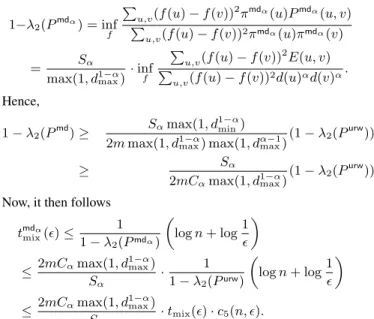
steps(mdα) = c5(n, )·2mCαmax(1, d
1−α
max) Sα
·tmix(),
wherec5(n, ) = 2c4(logn+ log(1/))for an appropriate con-stantc4. Furthermore if we run until we see
queries(mdα) = K(c5(n, ) + 1)· 2m Sα 2 Cα·tmix(), many queries, then for any constantK≥1, we would have taken steps(mdα)with probability at least1− 1
PROOF. Applying the variational characterization (2) toPmd
α ,
and using its definition, we obtain
1−λ2(Pmdα) = inf f P u,v(f(u)−f(v)) 2 πmdα(u)Pmdα(u, v) P u,v(f(u)−f(v))2πmdα(u)πmdα(v) = Sα max(1, d1max−α) ·inf f P u,v(f(u)−f(v)) 2 E(u, v) P u,v(f(u)−f(v))2d(u)αd(v)α . Hence, 1−λ2(Pmd)≥ Sαmax(1, d 1−α min)
2mmax(1, d1max−α) max(1, dα−max1)
(1−λ2(Purw))
≥ Sα
2mCαmax(1, d1max−α)
(1−λ2(Purw))
Now, it then follows tmdα mix()≤ 1 1−λ2(Pmdα) logn+ log1 ≤ 2mCαmax(1, d 1−α max) Sα · 1 1−λ2(Purw) logn+ log1 ≤ 2mCαmax(1, d 1−α max) Sα ·tmix()·c5(n, ).
Note that in expectation after the underlineurwis mixed we make P
uP[X=u]d(u) α−1
max(1, d1max−α) =2Smαmax(1, d
1−α
max)steps for every query in expectation. So we have that if we run
2m Sα
2 Cα·
tmix()·(c5(n, ) + 1)queries the expected number of steps is at least
2m
SαCαmax(1, d 1−α
max)·tmix()·c5(n, ). So by Markov inequality by runningK times those many queries with probability at least
1− 1
K we have taken enough steps.
5.3
Metropolis–Hastings sampling
To sample a nodeuwith probability proportional tod(u)α
us-ing Metropolis–Hastus-ings, we define a new random walkPMHαas follows: PMHα(u, v) = min 1 d(v), d(v)α d(u)α+1 {u, v},∈E 1− X v∈Γ(u) PMHα(u, v) u=v, 0 otherwise. (12)
Now we can upper bound the number of steps and the number of queries forMHα. We state the following theorem without proof.
THEOREM 19. To generate an-approximate sample fromΠ0
, the number of steps and queries needed are given by
steps(MH) = c7(n, )·2mCαdmax
Sαdαmin
·tmix(),
wherec7(n, ) =c6(logn+log(1/))for an appropriate constant
c6.
6.
EXPERIMENTS
In order to study the query complexity empirically, we formu-lated the following set of questions:
• How does the mixing rate of the three algorithms depend on the number of queries performed by the walk?
• How do the algorithms perform in terms of estimating basic network statistic, e.g., graph size, average degree, and clus-tering coefficient?
6.1
Datasets
We use the following publicly available datasets, all collected from snap.stanford.edu. Enron and Gnutella are undi-rected network generated from email-exchanges and peering re-lation in the p2p network. DBLP results from co-authorship of papers, whileweb-NDis the undirected version of the web graph of an university. Table 6.1 describes the basic statistics of these networks.
Dataset Nodes Edges
Enron 34K 180K
Gnutella 62K 148K
DBLP 317K 1049K
web-ND 325K 1117K
Table 1: Network statistics.
6.2
Algorithms
For each of these networks, we run random walks to try to sam-ple from the target distributionΠ0
andΠ2
. We run the random walks forrejandmdfor the two target distributions in the same manner as described in Algorithm 1 and (6) respectively. For each of the walks, we calculate the number of distinct query nodes touched, assuming that a node visited before could have been cached by the algorithm. ForMH, we run two variants of the walk. The naive variant, denoted in figures asMH, penalizes all self-loops ofMH
as queries, since in order to reject a transition, the walk has to visit the proposed candidate in order to obtain its degree. The optimistic variant, denoted in figures asMH+, assumes that neighbor degrees are stored in each node, and so rejecting proposed candidates does not result in additional queries.
For each network, we run200random walks of each type, and for at most1millionsteps. Each walk (for each type) starts at the same node, but is otherwise independent. Note that since we want to examine empirical convergence rate, the results could pos-sibly depend on the starting point, however, after examining100
randomly chosen starting points, we did not observe any effective change in the plots and hence report the plots with only one arbi-trary starting vertex.
Note that there are a number of heuristic convergence statistics that are often used in practice in order the judge whether a Markov chain has converged. These techniques, however, are useful mostly when the actual stationary distribution is not accessible.
6.3
Results
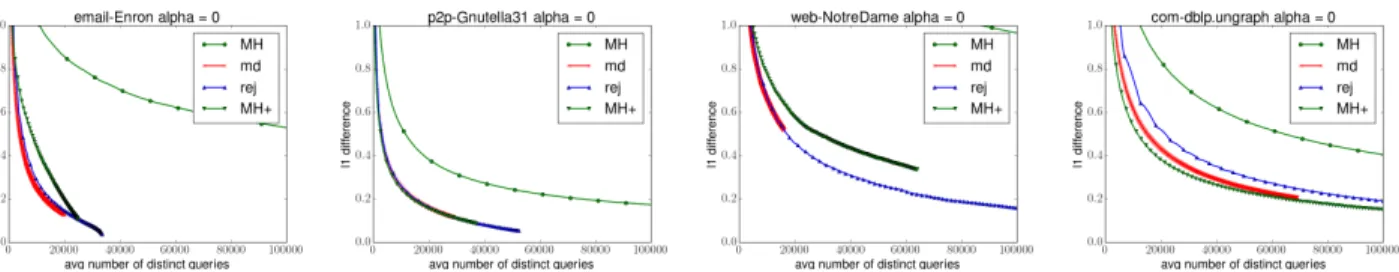
Figure 1 shows the`1 difference betweenΠ0 and the empiri-cal frequency distributions of each of the walks, when the number ofqueriesis as denoted by thex-axis. MHtypically performs worse than the other alternatives, which are more or less similar to each other, withmdbeing slightly better thanrejin most cases. However, augmentingMHwith the neighbor degree information (MH+) makes it converge faster than all the other alternatives.
Figure 1 shows the similar plot for the targetΠ2. Note that in this case, even the naiveMHoften performs better thanrej, in spite of the lower bound in Theorem 15. This leaves an open question of whether the lower bound can be refined in terms of a specific graph statistic which, although could be bad in the worst case, does have a “reasonable” value for real networks.
The`1 difference between distributions is an extremely strong criteria, and as we see in the above plots, it takes a significant num-ber of steps for this difference to be sufficiently less than1. Hence,
Figure 1: L1 difference fromΠ0 for each of the four datasets 1)Enron2)Gnutella3)web-NDand 4)DBLP. X-axis is number of
queriesused.
Figure 2: L1 difference fromΠ2 for each of the four datasets 1)Enron2)Gnutella3)web-NDand 4)DBLP. X-axis is number of
queriesused.
Figure 3: Relative error in estimating|V|for each of the four datasets 1)Enron2)Gnutella3)web-NDand 4)DBLP. X-axis is number ofqueriesused, sampled from the walks at a gap of1000. Note that Y-axis are differently sized.
Figure 4: Relative error in estimating average degree for each of the four datasets 1)Enron2)Gnutella3)web-NDand 4)DBLP. X-axis is number ofqueriesused. Note that Y-axis are differently sized.
Figure 5: Global clustering coefficient estimate for each of the four datasets 1)Enron2)Gnutella3)web-NDand 4)DBLP. X-axis is number ofqueriesused. The walk used was forΠ2. Note that Y-axis are differently sized.
we next compare the performance of the random walks in terms of the quality of samples that they provide after a fixed number of steps. In order to create these samples, we first discard an initial part of each walk. We then take samples after every1000queries have been performed by each walk.
In order to estimate the total size of the network, we use the es-tablished birthday paradox method. If in a (repeated) sample of size s, we getCcollisions, then we estimaten=|V|asnˆ= s2
2C. Note
that there are two types of errors in the random walk sampling— due to the walks not having converged, and due to the correlation in the samples. Since we discard an initial prefix, we mostly see the effect of the latter. Figure 3 shows the relative error (|n−nn|ˆ for estimaten) for sampling by each walk. Again, the behavior ofˆ rej
andmdare mostly same, withMHoccasionally performing much worse than the others.
Estimating average degree is also easy once we have uniform sampling of nodes. Figure 4 plots the relative error incurred by the different walks. Other than the fact all the algorithms perform badly onweb-ND, there is little to distinguish them in this metric. The global clustering coefficient is defined as the ratio of the number of triangles to the number of length2paths. In order to estimate the global clustering coefficient, we use walks designed forΠ2and use the same sampling method described above. Each such node then chooses a pair of neighbors and checks whether it is a triangle, (1/6th of) the fraction that forms a triangle is then returned. They-axis in Figure 5 plots the absolute estimates rather than the errors. For the two smaller networks we do reach close the number of triangles. For the larger networks, there is a gap indicating that we need more samples for good relative error bound. Again, the performances of the different walks are more or less similar.
7.
RELATED WORK
Generating a uniform node in a network has been studied in a number of papers. Most of the work, unfortunately, has been em-pirical and are not focused on the query complexity aspects. Gjoka et al. [7] modified the simple random walk to induce the uniform distribution on nodes as the stationary distribution; their main idea is to use a version of the Metropolis–Hastings algorithm for unbi-asing. See also the work of Stutzbach et al. [23]. Bar-Yossef et al. [1, 2] proposed themdalgorithm in order to unbias the distri-bution induced by the uniform random walk. However, they did not give theoretical bounds on the performance ofmd. Subsequent work such as that of Li et al. [17] obtained practical algorithms that perform better thanMHandmd, but once again did not analyze the performance of these algorithms in terms of their query complexity. Very recently, Nazi et al. [19] proposed to combine random walk with a proactive estimation step in order to reduce the long burn-in period typical with random walks.
Sampling in the context of network parameter estimation has been extensively studied in several papers. In particular, for the problem of estimating the size of the networks, sampling and col-lision counting are classical methods; see the work of Katzir et al. [14] and Hardiman and Katzir [9]. Another problem that has attracted a lot of attention is that of estimating clustering coeffi-cients [9]. All of these works are based on simple uniform random walks on the network. Ye and Wu [24] also consider the social network size estimation problem; while they assume the ability to uniformly sample a node, it is easy to argue that this is an unrealis-tic assumption. Cooper, Radzik, and Siantos [5] also used random walk methods for estimating network parameters, but they go be-yond collisions by actually using the return times for estimation.
Ribeiro and Towsley [20] used multidimensional random walks for the sampling and estimation problems. Leskovec and Falout-sos [15] posed the problem of obtaining a representative sample of the network to approximate various properties of the original net-work such as average shortest path, centrality, etc.
Non-uniform sampling has also been used to estimate certain network parameters. The main reason is that they are sometimes provably more powerful than uniform sampling. Katzir et al. [13] gave a method to estimate the size of networks and size of subpop-ulations using degree-biased sampling (i.e., according toΠ1) and counting collisions in the samples collected. Dasgupta et al. [6] used degree-biased sampling to estimate the average degree of a graph. They showed that degree-biased sampling can improve the query complexity of estimating the average degree almost exponen-tially. In a recent work, Seshadri et al. [21] showed that sampling nodes with probability proportional to the square of the degree (i.e.,
Π2
) is a provably better way for estimating the number of triangles in a network; see also [12].
Zhou et al. [25] modify the simple random walk in order to re-duce the mixing time of the walk. Boyd et al. [3] considered the problem of modifying edge probabilities to achieve the fastest mix-ing time; this turns out to be a semi-definite program. Even though both these works try to reduce the mixing time, it is unclear if they can of any help in improving the query complexity of sampling.
An excellent bibliography of sampling in networks can be found inwww.utdallas.edu/~emrah.cem/links.html. A com-prehensive survey on techniques to bound the mixing time of a Markov Chain is [8].
8.
CONCLUSIONS
In this paper we studied the query complexity of sampling in a graph. Focusing on the uniform sampling question, we proved near-tight bounds for three popular random-walk based algorithms. The techniques we use to show the query complexity bound, via the variational inequality, might be of independent interest since typi-cal analysis in random walks focuses more on the number of steps than on the number of queries. Our work poses a natural intrigu-ing open problem: is the query complexity of samplintrigu-ing a uniform at random nodeΩ(davg·tmix)? An affirmative answer will essentially mean that one has to either make additional assumption on the input graph or resort to heuristics to get any improvements. A negative answer, which seems less plausible, would be very surprising!
Acknowledgments. We thank the reviewers for many useful sug-gestions.
9.
REFERENCES
[1] Z. Bar-Yossef, A. C. Berg, S. Chien, J. Fakcharoenphol, and D. Weitz. Approximating aggregate queries about Web pages via random walks. InVLDB, pages 535–544, 2000.
[2] Z. Bar-Yossef and M. Gurevich. Random sampling from a search engine’s index.J. ACM, 55(5), 2008.
[3] S. Boyd, P. Diaconis, and L. Xiao. Fastest mixing Markov chain on a graph.SIAM Review, 46(4):667–689, 2004. [4] J. Cheeger. A lower bound for the smallest eigenvalue of the
Laplacian. In R. C. Gunning, editor,Problems in Analysis (Papers dedicated to Salomon Bochner), pages 195–199. Princeton Univ. Press, 1970.
[5] C. Cooper, T. Radzik, and Y. Siantos. Estimating network parameters using random walks. InCASoN, pages 33–40, 2012.
[6] A. Dasgupta, R. Kumar, and T. Sarlós. On estimating the average degree. InWWW, pages 795–806, 2014.
[7] M. Gjoka, M. Kurant, C. Butts, and A. Markopoulou. Walking in Facebook: A case study of unbiased sampling of OSNs. InINFOCOM, pages 1–9, 2010.
[8] V. Guruswami. Rapidly mixing Markov chains: A comparison of techniques.A Survey, 2000. [9] S. J. Hardiman and L. Katzir. Estimating clustering
coefficients and size of social networks via random walk. In
WWW, pages 539–550, 2013.
[10] W. K. Hastings. Monte Carlo sampling methods using Markov chains and their applications.Biometrika, 57(1):97–109, 1970.
[11] M. Hildebrand. Random walks on random simple graphs.
Random Structures & Algorithms, 8(4):301–318, 1996. [12] M. Jha, C. Seshadhri, and A. Pinar. Path sampling: A fast
and provable method for estimating 4-vertex subgraph counts. InWWW, pages 495–505, 2015.
[13] L. Katzir, E. Liberty, and O. Somekh. Estimating sizes of social networks via biased sampling. InWWW, pages 597–606, 2011.
[14] L. Katzir, E. Liberty, and O. Somekh. Framework and algorithms for network bucket testing. InWWW, pages 1029–1036, 2012.
[15] J. Leskovec and C. Faloutsos. Sampling from large graphs. InKDD, pages 631–636, 2006.
[16] D. Levin, Y. Peres, and E. Wilmer.Markov Chains and Mixing Times. American Mathematical Society, 2009.
[17] R.-H. Li, J. X. Yu, L. Qin, R. Mao, and T. Jin. On random walk based graph sampling. InICDE, pages 927–938, 2015. [18] L. Lovász and P. Winkler. Efficient stopping rules for
Markov chains. InSTOC, pages 76–82, 1995.
[19] A. Nazi, Z. Zhou, S. Thirumuruganathan, N. Zhang, and G. Das. Walk, not wait: Faster sampling over online social networks.PVLDB, 8(6):678–689, 2015.
[20] B. Ribeiro and D. Towsley. Estimating and sampling graphs with multidimensional random walks. InIMC, pages 390–403, 2010.
[21] C. Seshadhri, A. Pinar, and T. G. Kolda. Wedge sampling for computing clustering coefficients and triangle counts on large graphs.Statistical Analysis and Data Mining, 7(4):294–307, 2014.
[22] A. Sinclair. Improved bounds for mixing rates of Markov chains and multicommodity flow.Combinatorics, Probability, & Computing 1, pages 351–370, 1992. [23] D. Stutzbach, R. Rejaie, N. G. Duffield, S. Sen, and W. Willinger. On unbiased sampling for unstructured peer-to-peer networks.IEEE/ACM Trans. Netw., 17(2):377–390, 2009.
[24] S. Ye and F. Wu. Estimating the size of online social networks. InSocialCom, pages 169–176, 2010. [25] Z. Zhou, N. Zhang, Z. Gong, and G. Das. Faster random
walks by rewiring online social networks on-the-fly. In