MASTER’S THESIS
POTENTIAL DEEP LEARNING
APPROACHES FOR THE PHYSICAL
LAYER
Author Rajapakshage Nuwanthika Sandeepani Rajapaksha Supervisor Prof. Nandana Rajatheva
Second Examiner Dr. Janaka V. Wijayakulasooriya
Engineering, Degree Programme in Wireless Communications Engineering, 59 p.
ABSTRACT
Deep learning based end-to-end learning of a communications system tries to optimize both transmitter and receiver blocks in a single process in an end-to-end manner, eliminating the need for artificial block structure of
the conventional communications systems. Recently proposed concept of
autoencoder based end-to-end communications is investigated in this thesis to validate its potential as an alternative to conventional block structured
communications systems. A single user scenario in the additive white
Gaussian noise (AWGN) channel is considered in this thesis. Autoencoder based systems are implemented equivalent to conventional communications systems and bit error rate (BER) performances of both systems are compared in different system settings.
Simulations show that the autoencoder outperforms equivalent uncoded binary phase shift keying (BPSK) system with a 2 dB margin to BPSK
for a BER of 10−5, and has comparable performance to uncoded quadrature
phase shift keying (QPSK) system. Autoencoder implementations equivalent to coded BPSK have shown comparable BER performance to hard decision
convolutional coding (CC) with less than 1 dB gap over the 0-10 dB Eb/N0
range. Autoencoder is observed to have close performance to the conventional
systems for higher code rates. Newly proposed autoencoder model as an
alternative to coded systems with higher order modulations has shown that autoencoder is capable of learning better transmission mechanisms compared to the conventional systems adhering to the system parameters and resource
constraints provided. Autoencoder equivalent of half-rate 16-quadrature
amplitude modulation (16-QAM) system achieves a better performance with
respect to hard decision CC over the 0-10 dB Eb/N0 range, and a comparable
performance to soft decision CC with a better BER in 0-4 dB Eb/N0.
Comparable BER performance, lower processing complexity and low latency processing due to inherent parallel processing architecture, flexible structure and higher learning capacity are identified as advantages of the autoencoder based systems which show their potential and feasibility as an alternative to conventional communications systems.
Keywords: autoencoder, deep learning, end-to-end learning, neural networks, communications, channel coding, modulation.
ABSTRACT
TABLE OF CONTENTS FOREWORD
LIST OF ABBREVIATIONS AND SYMBOLS
1 INTRODUCTION 7
1.1 Motivation and Thesis Objectives . . . 8
1.2 Thesis Structure . . . 9
2 BACKGROUND AND LITERATURE 10 2.1 Potential of Deep Learning for the Physical Layer . . . 10
2.2 Deep Learning Basics . . . 11
2.3 Deep Learning Libraries . . . 12
2.4 Literature Review . . . 13
2.4.1 Deep Learning based Block Structured Communications . . . 13
2.4.2 Deep Learning based End-to-End Communications . . . 15
3 END-TO-END LEARNING OF UNCODED SYSTEMS 18 3.1 End-to-End Learning of a Communications System. . . 18
3.1.1 System Model . . . 18
3.1.2 Autoencoder for End-to-End Learning . . . 19
3.2 Autoencoder Implementation for Uncoded Communications Systems . . . 20
3.3 Results and Analysis . . . 21
4 END-TO-END LEARNING OF CODED SYSTEMS 26 4.1 System Model . . . 26
4.1.1 Baseline for Comparison . . . 27
4.2 Autoencoder Implementation for Coded Communications Systems with BPSK Modulation for AWGN Channel . . . 27
4.2.1 Implementation . . . 27
4.2.2 Results and Analysis . . . 28
4.3 Autoencoder Implementation for Coded Communications Systems with Higher Order Modulations . . . 35
4.3.1 Implementation . . . 35
4.3.2 Effect of Model Layout and Hyperparameter Tuning for the Performance . . . 37
4.3.3 Results and Analysis . . . 38
4.3.4 Processing Complexity . . . 43
4.3.5 Comparison with 5G Channel Coding and Modulation Schemes . . . . 45
5 CONCLUSION AND FUTURE WORK 46 5.1 Summary and Conclusion . . . 46
5.2 Future Work . . . 48
6 REFERENCES 49
This thesis is focused on potential deep learning approaches for the physical layer as a part of the High5 and MOSSAF projects at the Center for Wireless Communications (CWC) of University of Oulu, Finland. I would like to express my sincere gratitude to my supervisor and mentor Prof. Nandana Rajatheva for the guidance, support, inspiration and encouragement given throughout the period of my master studies. I am also grateful to Academy Prof. Matti Latva-aho for providing me the opportunity to join and contribute to the High5 and MOSSAF projects. Also I would like to thank project manager Dr. Pekka Pirinen and the other colleagues at CWC for their support in my research. I would also like to express my gratitude to Matti Isohookana, the coordinator of Double Degree Master’s Program, for his support and guidance throughout the past year.
I am also thankful to Dr. Janaka V. Wijayakulasooriya, my supervisor from University of Peradeniya, Sri Lanka, for the support given. Also I would like to thank all the lecturers from University of Peradeniya for their contribution in making the inaugural Double Degree Master’s Programme a success.
Finally I would like to express my sincere gratitude to my mother, father and brother for their immense love, support and encouragement provided throughout my life.
Oulu, 30th July, 2019
Acronyms
1D One-Dimensional
2D Two-Dimensional
3GPP 3rd Generation Partnership Project 4G Fourth Generation
5G Fifth Generation
ANN Artificial Neural Network
ASIC Application-Specific Integrated Circuit AWGN Additive White Gaussian Noise
BAIR Berkeley Artificial Intelligence Research BER Bit Error Rate
BLER Block Error Rate
BPSK Binary Phase-Shift Keying CC Convolutional Coding
CNN Convolutional Neural Networks
CP Cyclic Prefix
CPU Central Processing Unit CSI Channel State Information
DL Deep Learning
DNN Deep Neural Network
GAN Generative Adversarial Network GD Gradient Descent
GPU Graphics Processing Units LDPC Low Density Parity Check LTE Long-Term Evolution
MASK M-ary Amplitude Shift-Keying MER Message Error Rate
MFSK M-ary Frequency Shift-Keying ML Machine Learning
MLP Multi Layer Perceptrons MMSE Minimum Mean Square Error MSE Mean Squared Error
NLP Natural Language Processing
NN Neural Network
NR New Radio
OFDM Orthogonal Frequency-Division Multiplexing QAM Quadrature Amplitude Modulation
QPSK Quadrature Phase-Shift Keying ReLU Rectified Linear Unit
RTN Radio Transformer Network SDR Software-Defined Radio SGD Stochastic Gradient Descent SNR Signal-to-Noise Ratio
URLLC Ultra-Reliable Low-Latency Communication
Symbols
Cn Set of complex n-vectors M Set of M messages
Eb/N0 Energy per bit to noise spectral density ratio
K Information block size
M Number of messages
Mmod Modulation order
N Size of the channel coded block
Pe Message error rate (MER)
R Rate (communication rate or code rate as applicable)
k Number of bits in in message s
kmod Number of bits per codeword when modulated with Mmod
order modulation
n Number of complex channel uses for transmitting message s
s Transmit message
ˆ
s Estimation of message s
x Transmitted signal vector
y Received signal vector
Wireless networks and related services have become critical and fundamental building blocks in the modern digitized world which have changed the way we live, work and communicate with each other. Emergence of many unprecedented services and applications such as autonomous vehicles, remote medical diagnostics and surgeries, smart cities and factories, artificial intelligence based personal assistants etc. are challenging the traditional communication mechanisms and approaches in terms of latency, reliability, energy efficiency, flexibility and connection density. Catering the stringent requirements arising from those different verticals requires a greater need for wireless system research with novel architectures, approaches and algorithms in almost all the layers of a communications system. Newly initiated fifth generation (5G) of mobile communication technology is expected to cater for these requirements revolutionizing everything so far in wireless-enabled applications [1].
As said, 5G brings most stringent requirements when catering to the advanced applications and services which will be supported by it. For example, ultra-reliable low-latency communication (URLLC), one category out of the three service categories defined in 5G, which perhaps may be the most challenging as it needs to meet two challenging and contradicting requirements: low latency and ultra-high reliability, requires end-to-end latency in range of 10 ms and very high reliability with 10−5 bit error rate (BER) in 1 ms period [2]. High reliability means that the channel estimation accuracy should be improved since the channel coding gain is small for the short packet lengths so that the loss, if any, caused by the channel estimation should be prevented as much as possible. It is to be achieved by advanced channel estimation techniques and by adding more resources to the pilots which again raises concerns with latency requirements as more pilots result in control overhead which affect the throughput and hence latency of the communications. Another concern is faster signal processing at the transmitter and receiver to achieve low latency requirements of URLLC. Therefore, for successful implementation of URLLC systems, all these factors need to be taken into consideration which requires novel architectures, approaches and algorithms in almost all the layers of the communication system.
Communications field is very rich of expert knowledge based on statistics, information theory and solid mathematical modelling capable of modelling channels [3], optimal signalling and detection schemes for reliable data transfer compensating for various hardware imperfections etc. especially for the physical layer [4]. However, existing conventional communication theories exhibit several inherent limitations in fulfilling the large data and ultra high rate communication requirements in complex situations such as channel modelling in complex scenarios, fast and effective signal processing in low latency systems such as URLLC, limited and sub-optimal block structures due to the fixed block structure of the communication systems etc. In recent history, there has been an increasing interest in deep learning approaches for the physical layer implementations due to certain advantages they possess which could be useful in overcoming the above challenges.
Fundamental requirement of a communications system is to reliably transmit a message from a source to a destination over a channel by the use of a transmitter and a receiver. In order to achieve an optimal solution in practice, transmitter and receiver are typically divided into chain of multiple independent blocks, each responsible for a specific sub-task such as source/channel coding, modulation/demodulation, channel estimation and equalization etc. [4]. Although this block structure enables individual analysis, optimization and controlling of each block, it is not clear that individually optimized processing blocks achieve the best possible end-to-end performance and that approach is known to be sub-optimal in certain instances [5].
On the other hand, a deep learning based communications system follows the initial definition of a communications system and tries to jointly optimize transmitter and receiver in an end-to-end manner without having a defined block structure [6], [5]. Such a simple and straightforward structure seems appealing to be implemented in practical systems with less computing complexity and processing delays, and with less power consumption, given that it can provide equal or better performance than the existing systems.
Based on the above motivations, the objective of this thesis is to study and develop deep neural network (DNN) based models for a communications system in an end-to-end manner with the intention of achieving similar or better performance in terms of block error rate (BLER)/ BER or reliability compared to the conventional communication algorithms, at the same time reducing the processing complexity and latency. The target is to see the potential of deep learning based approaches to replace or assist the conventional communication algorithm implementations in the physical layer when trying to achieving the 5G specifications.
Simple and flexible structure of autoencoder based communications system [5] and its capability to learn adjusting to the given channel model and system parameters has inspired us to study about the autoencoder based end-to-learning of communications systems. In this thesis, we extend the previous research done in autoencoder based end-to-end learning of communications systems comparing the performance of deep learning models with their equivalent conventional implementations with different modulation schemes and code rates to understand the potential of deep learning based end-to-end communications as an alternative to conventional implementations. Scope of research conducted for this thesis is limited to single user implementations over the AWGN channel.
Main objectives of the thesis can be stated as follows.
• Perform a literature review about the 5G physical layer requirements and specifications, get an understanding about the challenges faced by current technologies and implementations.
• Conduct a thorough literature review on deep learning concepts for the physical layer and identify appropriate deep learning approaches as alternatives for the conventional communications systems.
system.
• Study the performance of the autoencoder based system as an alternative to uncoded communications systems comparing performance for different modulation schemes.
• Study the performance of the autoencoder based systems in comparison to equivalent conventional coded communications systems.
• Improve the existing autoencoder model or develop a new model to enable implementing systems equivalent to coded systems with different higher order modulation with comparable performance to the existing conventional systems.
• Analyse the processing complexity of autoencoder based systems and equivalent conventional systems in order to get an overall understanding for comparing the performance capability and computational complexity which are important parameters when proposing deep learning based implementations as alternatives to conventional communications systems.
1.2 Thesis Structure
The thesis is structured into five chapters. In this chapter we have given an overview about requirements and challenges which are needed to be addressed by future communications systems and have discussed our motivations to look into deep learning based approaches for the physical layer communication blocks. In the second chapter we present the background and literature related to the thesis work. There we discuss the potential of deep learning for the physical layer in detail, along with deep learning basics which are relevant in the context of studied literature and the thesis work. Then we present the literature review, explaining the existing work on deep learning based block structured communications and deep learning based end-to-end communications.
In the third chapter, we discuss the autoencoder concept for end-to-end learning of communications systems and analyse the performance of the autoencoder based end-to-end system proposed by [5] in comparison to conventional uncoded systems with different modulation schemes. In the fourth chapter we analyse the performance of the autoencoder based end-to-end learning system in comparison to conventional coded systems with different modulation schemes. There, we also present a new autoencoder model to cater for implementing equivalent autoencoder counterpart of coded systems with higher order modulation schemes with a comparable BER performance to the baseline systems compared. In the last chapter we present the conclusions of our research findings along with future directions for improvements.
2 BACKGROUND AND LITERATURE
There have been attempts to apply machine learning (ML) for the physical layer for few decades where researchers have proposed ML based algorithms for different sub tasks in the physical layer such as modulation recognition [7], [8], encoding and decoding [9], [10], channel modelling and identification [11], channel estimation and equalization [12], [13], [14] etc. However, it is seen that ML has not been commercially used due to the fact that ML algorithms do not have enough learning capability to cater for the complex task of handling physical channels.
It is believed that introduction of deep learning (DL) to the physical layer could bring further performance improvements to the existing ML approaches, eliminating the limitations faced by conventional ML algorithms, due to the characteristics it has such as deep modularization which enhances feature extraction and structural flexibility to a great extent compared to ML algorithms [15]. Specifically, DL-based systems could be used to automatically learn features from raw data instead of manual feature extraction where flexible adjustment of model structures via hyperparameter tuning is possible in order to optimize end-to-end performance of the system.
In this chapter we discuss the potential of applying DL for the physical layer which has created a great interest among the research community to study DL-based approaches for the physical layer. We then present a basic overview about the basic DL concepts where a detailed description of different DL concepts is available in Appendix 1. An overview of different DL libraries is also presented. Finally, we present a detailed overview of selected literature which have proposed new DL-based approaches in the physical layer of the communication systems.
2.1 Potential of Deep Learning for the Physical Layer
• Signal processing algorithms in communications are mostly based on statistics and information theory and are often proved to be optimal for tractable mathematical models. However, practical systems have many imperfections and non-linearities which may be difficult to fully capture from mathematical models [5].
On the other hand, deep networks have been proven to be universal function approximators [16] with a better learning ability and thus can be used to model communications systems despite complex channel conditions and hardware imperfections that are mathematically difficult to model. The “learned” algorithms in DL-based communication systems are represented by the weights learned in DL models which have been optimized for end-to-end performance through training, instead of requiring well defined mathematical models or expert algorithms [15].
• DL approaches essentially require to cater for handling large amounts of data due to their nature of distributed and parallel processing architectures, which enables computational speed and processing capacity. DL systems have a great potential in producing a considerable computational throughput through parallelized processing architectures [15].
• Since the execution of neural networks (NNs) can be highly parallelized on concurrent architectures and implemented with low-precision data types, it is
observed that these “learned” algorithms could be executed faster and at lower energy cost than their manually “programmed” counterparts [5]. Parallel processing architectures with distributed memory architectures such as graphics processing units (GPUs) and specialized chips for NN inferences, are proved to be very energy efficient and capable of providing considerable computational throughput when fully utilized by parallel implementations [5].
• DL based communication systems do not require the conventional block structure to achieve the global performance as they target optimizing the end-to-end performance instead of explicitly optimizing the individual blocks. Thus, the artificial block based structure will be not required if the whole communications system is based on a DL approach, and there is potential to improve the overall performance if such an end-to-end system is implemented.
• Recent development of dedicated DL libraries, tools and frameworks such as TensorFlow [17], PyTorch [18], Caffe [19] etc. enable fast experimentation and prototyping of DL models and quick and easy deployment of them enabling applying DL-based approaches for a wide variety of application areas.
2.2 Deep Learning Basics
DL is a branch of ML which enables an algorithm to predict, classify or make decisions based on data without being explicitly programmed. DL uses multiple layered structures and nonlinear processing units to hierarchically extract higher level features from raw input data in order to optimize a given target objective in contrast to the conventional ML algorithms which depend on manually extracted features by domain experts, thus has a wide learning capacity. DL expands in supervised, unsupervised and reinforcement learning domains similar to the ML algorithms. While DNNs are the most known DL models, other deep architectures such as deep Gaussian processes, neural processes, and deep random forests can also be regarded as deep models which consist of multiple layered structures [20].
The history of DL goes back to 1940s-1960s where the development of theories of biological learning and implementations of the first models such as the perceptron which allowed training of a single neuron were happened [21]. However, it was only in late 1980s where NNs gained interest after Rumelhart et al. [22] showed the possibility of training NNs consisting of one or two hidden layers using back propagation [20]. DL has gained a much wider interest and a rapid growth in the past 15-20 years due to the technological advancements like GPUs, software libraries and due to big data etc. which have eliminated computational limitations of training DL models, resulting in using DL-based approaches in a wide variety of applications [20].
Feedforward neural networks, convolutional neural networks (CNNs), autoencoders and generative adversarial networks (GANs) are some of the different types of DL models which are mainly used in literature under the scope of this thesis. A detailed overview about those DL concepts are presented in Appendix 1 along with an overview about the deep network training process. There we have mainly referred [21] for the theoretical parts related to DL concepts.
2.3 Deep Learning Libraries
Building a DL model from the scratch is a complex task and requires a great effort as it requires definitions of forwarding behaviours and gradient propagation operations at each layer and implementing efficient and fast optimization algorithms for model training, in addition to CUDA coding for GPU parellelization. In recent years, DL has gained a great momentum and popularity being used in quite many application areas such as image and video recognition, speech recognition and natural language processing (NLP) etc. This continuously-growing usage and popularity of DL has resulted in development of numerous tools, algorithms and dedicated libraries which make it easy to build and train large NNs. Most of these tools allow high level algorithm definition in various programming languages or configuration files, automatic differentiation of training loss functions through arbitrarily large networks, and compilation of the network’s forwards and backwards passes into hardware optimized concurrent dense matrix algebra kernels [5]. They are built with massively parallel GPU architectures enabling GPU acceleration which makes faster processing of model training routines of large networks with huge amounts of data. A brief summary of some of the widely used libraries is given below.
• TensorFlow
Created by the Google Brain team, TensorFlow is an open source library for numerical computation and large-scale machine learning that operates at large scale and in heterogenous environments [17]. TensorFlow uses dataflow graphs to represent computation, shared state, and the operations that mutate that state. It maps the nodes of a dataflow graph across many machines in a cluster, and within a machine across multiple computational devices, including multicore cetnral processing units (CPUs), general-purpose GPUs, and custom-designed application-specific integrated circuits (ASICs) known as Tensor processing units (TPUs) [17]. TensorFlow supports multiple languages to create DL models. Some of the languages that it supports are Python, C++, Java, Go, R. Currently, the best-supported client language is Python with detailed documentation and tutorials. Keras [23], Luminoth and TensorLayer are some of the dedicated DL toolboxes which are built upon TensorFlow, which provide higher-level programming interfaces. Keras is the main tool which we have used to implement the DL models we have proposed in this thesis, as it has a very user friendly and highly customizable interface which enables quick and easy prototyping for experimenting.
• PyTorch
PyTorch [18] is a Python based open source DL library inspired by Torch. It is a framework built to be flexible and modular for research, with the stability and support needed for production deployment. PyTorch has been primarily developed by Facebook’s artificial intelligence research group. PyTorch is one of the preferred DL research platforms built to provide maximum flexibility and speed. It is known for providing two of the most high-level features; namely, tensor computations with strong GPU acceleration support and building deep neural networks on a tape-based autograd systems designed for immediate and python-like execution. PyTorch has a growing popularity among the research community since building NNs in PyTorch is straightforward.
• Caffe
Caffe is a dedicated DL framework made with expression, speed, and modularity in mind. It is developed by Berkeley artificial intelligence research (BAIR) [19] and by community contributors. It allows to train NNs on multiple GPUs within distributed systems, and supports DL implementations on mobile operation systems, such as iOS and Android [20].
2.4 Literature Review
Recent studies have proposed DL based approaches to improve the performance of the communications systems, motivated by the potential of DL for the physical layer applications (Section 2.1), which are based on and enabled by the concepts and technologies as discussed in Appendix 1. In literature, two main approaches are proposed, where DL is either used to enhance and optimize certain blocks of the conventional communication system as an alternative to the existing processing algorithms in each block (such as modulation recognition, channel encoding and decoding, channel estimation and detection etc.) or to completely replace the total block based communication system with a DL based architecture which optimizes the end-to-end performance of the system without a specific block structure like in conventional systems. In this section, we present an overview of selected literature which has DL based applications that cover the aforementioned two approaches.
2.4.1 Deep Learning based Block Structured Communications
As noted earlier, the fundamental requirement of a communications system is reliable transmission of a message from source to destination over a communications channel. In practice, a conventional communications system is constructed as a block structure in order to achieve an optimal solution for this task where different algorithms which are based on expert knowledge have been developed over decades in order to optimize each individual block of the communications system. The structure of a standard communications system is shown in Figure 2.1 which consists of source/channel coding and decoding, modulation and demodulation, channel estimation and signal detection.
Over the years, studies have proposed to use conventional machine learning approaches such as support vector machines (SVMs) and small feedforward NNs as alternative implementations to cater for those individual tasks [15]. With the development of DL algorithms and architectures, in recent years DL based approaches have been introduced into different processing blocks of the communications systems as alternatives to conventional algorithms such as modulation recognition [5], channel encoding and decoding [24], [25], [26], [27], [28], [29] and channel estimation and detection [30], [31], [32], [33].
Source Destination Source Coding Source Decoding Channel Coding Channel Decoding Modulation Demodulation Detection Channel Estimation RF Receiver RF Transmitter Channel
Figure 2.1. Structure of a classical communications system.
These DL based algorithms are expected to be more effective in complex communications scenarios where the learning capability of DL can be leveraged to adapt to different complex channel conditions, complex operating environments etc. Also DL based approaches would be more useful in instances where reduced the computational complexity and processing overhead are preferred. In this section, we present some of the examples which use DL applications for different processing blocks such as signal detection and modulation recognition.
Deep Learning based Joint Channel Estimation and Signal Detection
In a conventional communications system, channel estimation and signal detection are two separate procedures executed at the receiver. Channel state information (CSI) is first estimated explicitly with the aid of the pilots prior to the detection of transmit symbols, and the estimated CSI is then used to detect/recover the transmitted symbols at the receiver. In [32], a DL based approach for joint channel estimation and signal detection in orthogonal frequency-division multiplexing (OFDM) systems is presented which uses DL to handle wireless OFDM channels in an end-to-end manner. In contrast to the existing conventional approach of explicit CSI estimation and symbol detection, the proposed DL based receiver implicitly estimates the CSI and recovers the transmitted symbols directly which is implemented as a five-layer fully connected DNN. They have initially trained an offline DNN model with generated data based on channel statistics and the trained model is then used to recover the online transmitted data directly. Their results have shown that the DL based approach performs in comparable to the minimum mean square error (MMSE) estimator. Proposed method shown to be more robust when a lesser number of pilots are used, cyclic prefix (CP) is omitted and when nonlinear clipping noise exists.
Deep Learning based Modulation Recognition
Modulation recognition which has the goal of differentiating different modulation schemes of received signals is an important task in the field of communications as it facilitates communication among the different communications systems, or interfering and monitoring enemies for military use. Modulation classification task has been studied over decades through the approach of expert feature engineering and either analytic decision trees or trained discrimination methods operating on a compact feature space, such as support vector machines, random forests, or small feedforward NNs. These approaches
consist of several common procedures such as preprocessing, feature extraction, and classification. Some researches have presented some advanced approaches using pattern recognition on expert feature maps, such as the spectral coherence function or α-profile, combined with NN-based classification.
In [34], an NN architecture is proposed as a modulation classifier to distinguish noise-corrupted band-limited modulated signals from 13 types of digital and analog modulation schemes. This approach manually extracts features from the signals including features which characterize digital or analog modulations and the basic parameters of signals such as amplitude, phase and frequency. Those features are fed to a four-layer NN to discriminate the different modulation schemes and two more two-layer NNs are used to estimate the levels of the M-ary amplitude shift-keying (MASK) and the M-ary frequency shift-keying (MFSK) modulations. The performance of these kind of feature engineered approaches strongly depends on the extracted features due to the limited learning ability of conventional NNs [15]. In several recent studies, the well admired learning capacity of DL is exploited to overcome the aforementioned limitations of feature based modulation classification approaches.
In [5], authors highlight the possibility to replace the artificial feature extraction with automatic learning of features from the raw data to optimize end-to-end performance, by using the superior learning capability of DNNs. They have proposed a convolutional neural network (CNN) based approach for modulation classification of single carrier modulation schemes based on sampled radio frequency time-series data. The CNN classifier is trained using a dataset of 1.2M sequences of 128 complex-valued baseband in-phase and quadrature (I,Q) samples corresponding to 10 different digital and analog single-carrier modulation schemes which have gone through a wireless channel with multipath fading effects and clock and carrier rate offset. Their results have shown that the CNN-based modulation classifier outperforms two other approaches: extreme gradient boosting with 1000 estimators and a single scikit-learn tree working on the extracted expert features, mainly in the low to medium signal-to-noise ratio (SNR) range where as in the high SNR range, CNN and boosted tree performance are similar.
2.4.2 Deep Learning based End-to-End Communications
In the previous section, we discussed several DL based approaches which are used as alternatives for one or two processing blocks of the conventional block structured communications system. However, when looking back to the original requirement of a communications system of transmitting a message from source to destination over a channel, even though the block structure enables individual analysis and controlling of each block, it can not be guaranteed that optimization of each block will always result in global optimization for the communication problem because end-to-end performance improvements can be achieved by joint optimization of two or more blocks.
A novel DL based concept has been introduced in recent history based on this thought process, which reformulates the communication task as an end-to-end reconstruction optimization task where the artificial block structure of the conventional communications system is no longer required. This novel concept is based on implementing the end-to-end communications system by an autoencoder system and the initial studies have shown that it has comparable performance to the conventional systems and also has shown that
the end-to-end method has great potential to be a universal solution for different channel models. In this section we discuss about that newly introduced concept of autoencoder based end-to-end communications and present details about some of very recent studies based on that.
Autoencoder based End-to-End Communications
Using the autoencoder concept for the communications system was first introduced in [6] and [5]. In [5], communications system is interpreted as an autoencoder and a new way of communications system design as an end-to-end reconstruction task which jointly optimizes the transmitter and receiver components in a single process is presented. They have shown that it is possible to learn transmitter and receiver implementations for a given channel model which are optimized for a desired loss function such as minimizing the BLER, using a DL model. They have implemented the transmitter, channel and the receiver as one DNN that can be trained as an autoencoder. The transmitter and receiver are represented as fully connected feedforward NNs and the AWGN channel between them is represented as a noise layer with the desired noise variance. Thus, the communications system can be seen as an autoencoder which tries to learn from the message s out of M
possible messagess∈M={1,2, ..., M}, to generate the representation of the transmitted signalxwhich is robust against the communication channel. At the receiver, the original messagesis reconstructed as ˆswith the lowest possible error by learning from the received signal y.
The whole network is trained end-to-end in order to achieve BLER performance. Their results have shown that the autoencoder based communications system achieves a comparable or better performance than standard BPSK with Hamming code, thus indicating that the system has learnt a joint coding and modulation scheme to minimize the BLER over the AWGN channel. Potential of application of the autoencoder based approach for channel models and loss functions where optimal solutions are not known is also noted in their study.
The potential of introducing communication expert knowledge to the autoencoder model which improves its performance, enables adjusting the DL architecture to accommodate different communication scenarios, and accelerates the DL model training phase is also shown in [5] by introducing the concept of radio transformer networks (RTNs). As noted by [5], RTNs enable carrying out predefined correction algorithms or “transformers” at the receiver (such as multiplication by a complex-valued number, convolution with a vector etc.) which can be used to reverse the channel effect occurred during signal transmission over the imperfect channel. The transformation layer can be fed with parameters learned by another NN and they can be integrated into the receiver in order perform symbol detection in a more effective manner by enabling integration of communication knowledge into the DL system. The authors have shown performance improvements and fast convergence of the model training than the plain autoencoder when RTN is used.
In [35], a more recent study carried out inspired by the initial findings of [5], the concept of autoencoder based end-to-end communications system is extended to an actual implementation showing the feasibility of over-the-air transmission. They have modeled, trained and run a complete communications system consisting of NNs using unsynchronized off-the-shelf software-defined radios (SDRs) and open source DL software
libraries. The limitation of short block lengths faced by the autoencoder models has been overcome by implementing mechanisms for continuous data transmission and receiver synchronization where a frame synchronization module based on another NN is implemented at the receiver to cater for the receiver synchronization. A two step training procedure based on transfer learning is used to overcome training the model over actual channels by finetuning the receiver part of the autoencoder to capture the effects of the actual channel including the hardware imperfections which are not initially included in the model. Comparison of the BLER performance of the “learned” system with that of a practical baseline have shown a comparable performance close to 1 dB. The study has thus validated the potential of actual implementation of autoencoder based communication systems.
Autoencoder for Multi-User
Extension of the autoencoder model to an adversarial network of multiple transmitter and receiver pairs competing for capacity is also presented in [5]. Simple two-user scenario is considered where the transmitter-receiver pair of each user attempt to communicate simultaneously over the same channel which leads to the interference channel where finding the best signalling scheme is known to be a well known long-standing research problem. In the two-user scenario, the overall system is trained to achieve conflicting goals at the receiver side, where each user tries to optimize the system to transmit their own messages in best possible accuracy. The system is represented as a multiple input-output NN and both transmitter-receiver pairs are jointly optimized with respect to a common performance metric, minimizing the weighted sum of both losses denoted by
L=αL1+ (1−α)L2 for some α ∈[0,1]. The results show that the autoencoder system
obtains similar of better BLER performance at the same communication rate than the uncoded quadrature amplitude modulation (QAM) schemes, thus validates the potential of application of autoencoder model in multi-user cases as well.
Over-the-Air Communications based on Adversarial Networks
In [36], channel autoencoder model is extended to enable end-to-end learning of the communications system when the channel response is unknown or cannot be easily modelled in a closed-form analytical expression. Previously, over-the-air channel autoencoders were implemented in two phases: initial pre-training based on a closed-form channel model to match the expected deployment scenario and fine-tuning the receiver part of the model to capture the actual channel effects [35]. In finetuning stage, optimization of only the receiver side of the network is possible as it is unable to back propagate through the black-box void of the radio channel. This limitation has been overcome in [36] by introducing an adversarial approach for channel response approximation where a learning based approach which does not require an analytic model for channel impairments is implemented. It is based on generative adversarial networks where the model tries to jointly optimize the two tasks of: 1) approximating the channel response of any arbitrary communications system, 2) learning an optimal encoding and decoding scheme that optimizes a given performance metric such as BLER. Their results show that such a model can result in an effective communications system which can achieve robust performance without the need of a close-form channel model or implementation.
3 END-TO-END LEARNING OF UNCODED SYSTEMS
As discussed in Chapter 2, end-to-end learning of a communications system using DL based autoencoder concept has drawn interest in recent research due to its simplicity, flexibility and its potential of adapting to complex channel models and practical system imperfections. In this thesis, we have extended the existing research on autoencoder based end-to-end learning of communications system in order to investigate its performance in different system configurations in order to understand the potential of autoencoder based end-to-end learning of communications systems.
In this chapter, we investigate the performance of autoencoder based end-to-end communications system in comparison with a conventional communications system when there is no channel coding applied. Thus, in this chapter we compare the performance of the autoencoder based system with conventional uncoded BPSK and QPSK performance over the AWGN channel.
First we explain the autoencoder concept and its application for end-to-end learning of communication systems as proposed by [5] formulating the system model and the autoencoder model layout. Then the implementation details are presented in Section 3.2 followed by results obtained for various configurations which is presented in 3.3. We have used the BER metric to compare the performance of the autoencoder and conventional implementations.
3.1 End-to-End Learning of a Communications System 3.1.1 System Model
A basic communications system consists of a transmitter, a channel and a receiver as shown in Figure 3.1. The transmitter wants to communicate a message s out of M
possible messages s ∈ M = {1,2, ..., M} to the receiver using n uses of the channel. It transmits a vector x of n complex symbols over the channel to send the message s to the receiver. Physical implementation at the transmitter imposes power constraints on
xsuch as an energy constraint x2
2 ≤n or an average power constraint E[x2i]≤1∀i.
Transmitter Channel Receiver
∈ ℂ
∈ ∈ ℂ ̂ ∈
Figure 3.1. Structure of a simple communications system.
Each message s can be represented in k = log2(M) number of bits. Thus, the
system operates in R=k/n [bits/channel use] communication rate. The channel causes distortions to the transmitted symbols and at the receiver upon reception of signal
y ∈ Cn, the receiver produces the estimate ˆs of originally transmitted message s. The
message error rate (MER) Pe can be defined as
Pe = 1 M X s P r(ˆs6=s|s). (1)
3.1.2 Autoencoder for End-to-End Learning
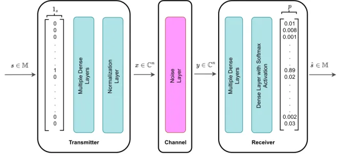
The above-mentioned simple communications system was first proposed to be interpreted as an autoencoder in [5]. As described in Appendix 1.C, an autoencoder is a type of ANN that tries to reconstruct its input at the output in an unsupervised manner. Thus, the communications system can be thought as an autoencoder which tries to reconstruct the transmit message at the receiver with a best possible minimum error. The encoder function and decoder function of the autoencoder model can be thought as the transmitter and receiver blocks of the system respectively. An autoencoder architecture which can be used to end-to-end learning of a communications system is shown in Figure 3.2.
Channel Transmitter Receiver M u lti pl e D e ns e L a ye rs N or m al iz a tio n L a ye r M u lti pl e D e ns e L a ye rs D e n se L a ye r w ith S o ft m a x A ct iv a tio n N o is e L a ye r 0.01 0.008 0.001 . . . . 0.89 0.02 . . . . . 0.002 0.03 0 0 0 . . . . 1 0 . . . . . 0 0 thesis-Page-7.svg https://www.draw.io/#G1Y8pZQEF3xZJkl4KwZlq6pr_kUvlmhhB8 1 of 1 7/30/2019, 10:26 AM
Figure 3.2. A communications system represented as an autoencoder.
There, the transmitter is implemented as a feedforward NN with multiple dense layers followed by a normalization layer to meet the physical constraints of transmit vector
x. Input s to the NN is an M-dimensional one-hot encoded vector 1s ∈ RM i.e., an
M-dimensional vector, the sth element of which is equal to one and zero otherwise.
Transmitter output is a 2n-dimensional vector which corresponds to n complex symbols transmitted in n channel uses by considering one half as real part and the other as the imaginary part. The channel is represented by an additive noise layer with a fixed variance β= (2REb/N0)−1, where Eb/N0 denotes the energy per bit (Eb) to noise power
spectral density (N0) ratio. The receiver is also implemented as a feedforward NN with
a single or multiple dense layers followed by an output layer with softmax activation whose outputp∈(0,1)M is a probability vector over all possible messages. The decoded
message ˆs corresponds to the element index of p which has the highest probability. This autoencoder can be trained end-to-end using stochastic gradient descent (SGD) or any other suitable optimization method on the set of all possible messages s ∈ M
3.2 Autoencoder Implementation for Uncoded Communications Systems
When investigating the potential of autoencoder implementation as an end-to-end communications system, we have first compared its performance with a simple transmitter-receiver structure without any channel coding applied. This section presents the implementation and the results obtained for the autoencoder based transmitter receiver system in comparison with the standard communications system with different modulation schemes.
We have implemented the autoencoder architecture proposed by [5] with slight modifications. The autoencoder models have been trained for different message alphabet sizes (M) with different communication rates and are compared with baseline BPSK and QPSK systems accordingly. The autoencoder was implemented as a fully connected feedforward NN. Different autoencoder architectures with different number of hidden layers and different activation functions were investigated. Table 3.1 lists out the activation function types and output dimensions in each layer of the selected optimum model layout where the autoencoder is constructed by sequentially combining the layers in the order listed in the table.
Table 3.1. Layout of the autoencoder model
Layer Output dimensions
Input M Dense-ReLU M Dense-ReLU M Dense-Linear 2n Normalization 2n Noise 2n Dense-ReLU M Dense-ReLU M Dense-Softmax M
Layers 1-5 compose the transmitter side of the system where the energy constraint of the transmit signals is guaranteed by the normalization layer at the end. Layers 7-9 compose the receiver side of the system where estimated message can be found from the output of the softmax layer. Noise layer in-between the transmitter and receiver side of the system acts as the AWGN channel.
Autoencoder is trained end-to-end over the stochastic channel model using SGD method with the Adam optimizer with learning rate = 0.001. Following approaches were taken to select Eb/N0 values for the AWGN channel during training:
• Training at a fixed Eb/N0 value (i.e., 5 dB or 8 dB etc.)
• Picking Eb/N0 values randomly from a predefined Eb/N0 range for each training
epoch
• Starting from a highEb/N0 value and gradually decreasing it along training epochs
Autoencoder model training and testing was implemented in Keras [23] with TensorFlow [23] as its backend. We have trained the models over 50 epochs using 1,000,000 randomly generated messages with Eb/N0 values for AWGN channel in model
training in three settings mentioned earlier. Testing the trained models were done with 1,000,000 different random messages for 0 dB to 8 dB Eb/N0 range and their BER
performance have been compared with the corresponding baseline systems.
We have tried out several autoencoder configurations which result in BPSK equivalent systems where communication rateR = 1 bit/channel use and QPSK equivalent systems where R = 2 bits/channel use. The message alphabet size M and number of channel uses n have been set accordingly in order to achieve the desired communication rate. Table 3.2 shows the autoencoder configuration parameters and their baseline systems which we have compared performance with. Total energy per message is kept same in both autoencoder system and baseline system in each scenario.
Table 3.2. Different autoencoder configuration parameters and their baseline systems used for performance comparison
Number of Complex Communication Equivalent messages (M) channel uses rate (R) modulation
per message (n) scheme
2 1 4 2 1 bit/channel use BPSK 8 3 16 4 4 1 16 2 2 bits/channel use QPSK 64 3 256 4
3.3 Results and Analysis BER performance
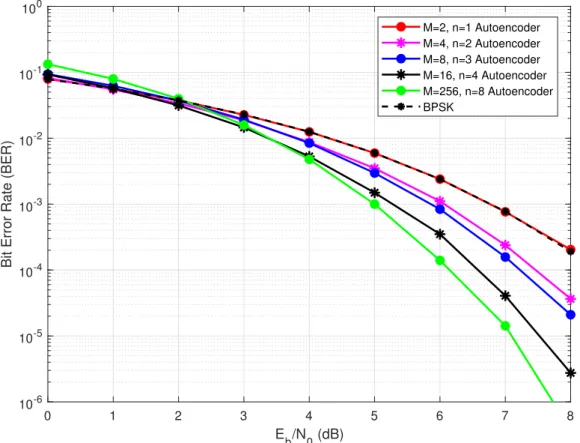
Figure 3.3 shows the BER performance of R = 1 systems compared with theoretical AWGN BER performance of their baseline BPSK scheme. It seems that all four autoencoder configurations have equal or better BER performance across almost full
Eb/N0 range except from 0 dB to 2 dB where some autoencoder systems have slightly
higher BER than BPSK system. It is interesting to see that the BER performance improves when the message alphabet size and number of channel uses per message increases even though communication rate is the same in all models. That is probably because the transmitted messages get some sort of temporal encoding since multiple channel uses are used to transmit a single message. When the number of channel uses per message increases, more flexibility and degree of freedom is there to formulate the
transmit symbols adjusting to the channel distortions and hence transmit symbols are more tolerant to errors and can be recovered at the receiver with less errors.
0 1 2 3 4 5 6 7 8 E b/N0 (dB) 10-6 10-5 10-4 10-3 10-2 10-1 100
Bit Error Rate (BER)
M=2, n=1 Autoencoder M=4, n=2 Autoencoder M=8, n=3 Autoencoder M=16, n=4 Autoencoder M=256, n=8 Autoencoder BPSK
Figure 3.3. BER performance of the R = 1 bit/channel use systems compared with theoretical AWGN BPSK performance.
However, it should be noted that this kind of a system has a certain delay when detecting and decoding received symbols at the receiver. That is, for a system with
M = 16 and n = 4, even though the communication rate of 1 bit/channel use gives the idea that we can decode 1 bit per each transmission at the receiver, we have to wait for four signalling instances to receive the complete message which consists of four symbols and then decode it so that it gives the 4 bits long message. While increasing M and n
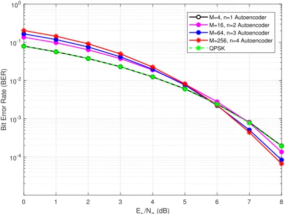
enables to have a lower BER for a system with a given communication rate, this delay in detection also needs to be taken into consideration when deciding M and n parameters. Figure 3.4 shows the BER performance of R = 2 systems compared with theoretical AWGN BER performance of their baseline QPSK scheme and there also we can observe that autoencoder has better BER performance than QPSK in higher Eb/N0 values.
However, it is seen that QPSK is better when Eb/N0 is in the low range between 0-5
0 1 2 3 4 5 6 7 8 E b/N0 (dB) 10-4 10-3 10-2 10-1 100
Bit Error Rate (BER)
M=4, n=1 Autoencoder M=16, n=2 Autoencoder M=64, n=3 Autoencoder M=256, n=4 Autoencoder QPSK
Figure 3.4. BER performance of the R = 2 bits/channel use systems compared with theoretical AWGN QPSK performance.
Learned Constellations
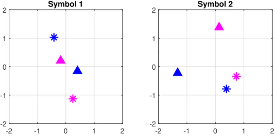
The autoencoder can be split to two parts: encoder and decoder, after training the model in end-to-end manner. Then the encoder part is implemented at the transmitter side which generates encoded symbols for each message to be sent over the channel and decoder part is implemented at the receiver which regenerates the messages from the received symbols. After completion of model training, encoder can generate all possible output signals for each message in the message alphabet. Figure 3.5 and Figure 3.6 show learned constellations for different systems we tested. When mapping 2n-dimensional output from the encoder model to the n-dimensional complex valued vector x, the odd indexed elements of x are taken as in-phase (I) components and even elements of x are taken as quadrature (Q) components. In the scatter plots, I and Q values are plotted in x- and y- axes respectively.
From the scatter plots in Figure 3.5, it can be seen that for the systems with M = 1,2 and 4 where n = 1, learned constellations are similar to BPSK, QPSK and 16-PSK constellations respectively, with some arbitrary rotations. For the M = 4, n = 2 system shown in Figure 3.6, we can observe that the model has learned unique constellation points for four messages in two symbols in order to minimize the symbol estimation error at the receiver. It can be seen that in the first symbol, points marked in “∗” have a maximum amplitude contrast in their in-phase amplitude values having high positive and negative values, and in the second symbol their signal points are closely located to each
other near zero. On the other hand, points marked in “4” have low amplitude values in the first symbol and high amplitude values in the second symbol. This arrangement has enabled the system to have a better a tolerance to channel distortions and has resulted in less symbol estimation errors at the receiver.
-2 -1 0 1 2 -2 -1 0 1 2 -2 -1 0 1 2 -2 -1 0 1 2 -2 -1 0 1 2 -2 -1 0 1 2
Figure 3.5. Scatter plots of learned constellations of [M = 2, n= 1], [M = 4, n= 1] and [M = 16, n= 1] systems respectively. -2 -1 0 1 2 -2 -1 0 1 2 Symbol 1 -2 -1 0 1 2 -2 -1 0 1 2 Symbol 2
Figure 3.6. Scatter plots of learned constellations for M = 4,n = 2 system. 4 messages are shown using 4 different markers in the plot.
Effect of Training Eb/N0 Values and Hyperparameter Tuning
During the model training it was observed that the deep model architecture and the model training parameters such as batch size and learning rate are critical factors for the performance of trained model. We have studied the BER performance of different model architectures which have single, double and multiple hidden layers in encoder and decoder parts of the autoencoder model, and it was observed that having multiple hidden layers improves accuracy than having a single hidden layer. This increased dimension parameter search space may help avoiding model convergence to sub-optimal minima during optimization as also pointed out by [5].
As noted in the previous studies also, the Eb/N0 value in which the model training
should be done plays a critical role in determining the performance of the trained model. We have tried different approaches to select training Eb/N0 values to see the impact of
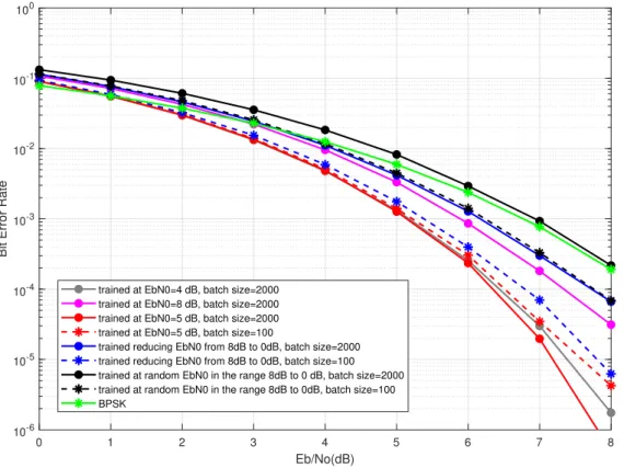
approaches is shown in Figure 3.7. For this, we have used M = 16, n= 4, R = 1 system configuration which is equivalent to BPSK.
0 1 2 3 4 5 6 7 8 Eb/No(dB) 10-6 10-5 10-4 10-3 10-2 10-1 100
Bit Error Rate
trained at EbN0=4 dB, batch size=2000 trained at EbN0=8 dB, batch size=2000 trained at EbN0=5 dB, batch size=2000 trained at EbN0=5 dB, batch size=100
trained reducing EbN0 from 8dB to 0dB, batch size=2000 trained reducing EbN0 from 8dB to 0dB, batch size=100 trained at random EbN0 in the range 8dB to 0 dB, batch size=2000 trained at random EbN0 in the range 8dB to 0dB, batch size=100 BPSK
Figure 3.7. BER performance for different training Eb/N0 values and different batch
sizes. M = 16, n= 4 (R = 1 bit/channel use) system used.
From the results, we could see that training at a fixed Eb/N0 value of 5 dB gave the
best BER performance. Increasing the training Eb/N0 seemed not that optimum as the
trained model was unable to perform well in lowEb/N0 values. When the trainingEb/N0
was selected to be too low, BER performance again degraded as the model seemed unable to capture the actual underlying patterns between inputs and outputs during training.
Different batch sizes were tried when training the models and it was observed that when training at a fixed Eb/N0 = 5 dB, a larger batch size of 2000 resulted in improved BER
performance compared to smaller batch sizes, while when training was done decreasing
Eb/N0 values along the training epochs, a smaller batch size around 50 or 100 gave better
BER performance than higher batch sizes. Overall, training at a fixedEb/N0 = 5 dB with
batch size = 2000 gave the best BER performance among the different configurations we tried.
4 END-TO-END LEARNING OF CODED SYSTEMS
In this chapter, we investigate the performance of autoencoder based end-to-end communications in comparison with conventional communications systems with channel coding applied. A conventional communications system consists of different blocks for channel coding/decoding and modulation/demodulation. Autoencoder based system does not have such explicit blocks, instead it tries to optimize the system in an end-to-end manner adhering to the configured system parameters such as input message size, number of channel uses per message and transmit signal power constraints. We use these system parameters to implement autoencoder models which are equivalent to conventional channel coded communications systems and compare their performance over the AWGN channel.
This chapter consists of two main sections. In Section 4.2, we use the same autoencoder layout used in Chapter 3 to implement systems equivalent to channel coded systems with BPSK modulation and compare the performance of autoencoder based systems and their equivalent conventional implementations. In Section 4.3, we propose a different autoencoder layout to enable implementing equivalent systems of channel coded systems with higher order modulations such as QPSK, 16-QAM etc. and compare performance of autoencoder based systems with their equivalent conventional implementations. We have mainly used BER metric to compare the performances.
4.1 System Model
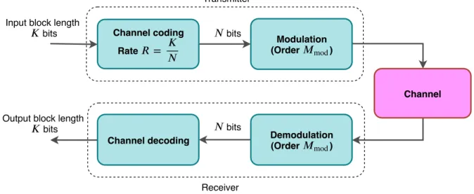
As shown in Figure 4.1, in a standard communications system, the information blocks are divided to blocks for ease of processing through different stages of the system. At the transmitter, information block of size K bits is fed to channel encoder where a block of size N is output after channel encoding, and the coding rate is defined as R =K/N.
Channel coding Rate = Demodulation (Order mod) Channel decoding Modulation (Order mod) Channel
Input block length
bits bits
bits Output block length
bits
Transmitter
Receiver
Figure 4.1. System model of a conventional communications system consisting of coding and modulation blocks.
Then the data block is fed to the modulator of order Mmod where the data bits are
divided into codewords of size kmod = log2(Mmod), and each codeword is mapped to
a point in the signal constellation with given amplitudes for the I,Q signals. At the receiver, the reverse process of the above happens where incoming symbols are mapped to codewords and the codewords are grouped serially to produce the block. It is then fed to the channel decoder where the N bit sized block is converted toK bit sized block after channel decoding which is the estimation of the transmitted information block.
In Section 4.2 and 4.3, the autoencoder model dimensions are selected in such a way that the above described network structure is preserved so that baseline system and autoencoder system can be compared.
4.1.1 Baseline for Comparison
For the channel encoding/decoding blocks in the standard communications system, we have used convolutional codes (CC) with Viterbi decoder, with hard decision decoding and soft decision decoding as the primary baseline comparison. CC with constrain length 7 is used when comparing the performance. For baseline systems, BER performance for different input block lengths withK ={200,400,800,1600,2000,4000}bits are evaluated to understand the effect of different block sizes for the conventional algorithms and to compare them with the autoencoder performance. Standard modulation schemes such as BPSK, QPSK, 16-QAM etc. are used in the modulation block. Conventional system was implemented in MATLAB [37] using the inbuilt functions and algorithms for coding, modulation and decoding functions and results obtained for the autoencoder models were compared with the obtained baseline results.
4.2 Autoencoder Implementation for Coded Communications Systems with BPSK Modulation for AWGN Channel
The same autoencoder model developed in Section 3.2 is used to compare the autoencoder model BER performance with the conventional coded system BER performance. Different rates R were achieved by changing ratio of the number of input bits k
and number of n channel uses in the autoencoder models accordingly, so that the models resulted in equivalent systems to conventional systems with code rates R =
{1/2,1/3,1/4}, and with BPSK modulation (Mmod = 2). The AWGN channel noise
variance is given by β = (2REb/N0)−1. This section presents the implementation and
the results obtained for the autoencoder based transmitter-receiver system in comparison with the standard communications system with different code.
4.2.1 Implementation
Autoencoder model was implemented, trained and tested in Keras with TensorFlow as backend similar to Section 3.2 and the model training was done in end-to-end over stochastic channel model using SGD with Adam optimizer with learning rate = 0.001. Same code rate values were achieved by implementing autoencoder models for different
messages sizesM ={2,4,16,256}and setting the number of channel uses (n) accordingly. Table 4.1 shows the model parameters for different simulations that were performed. For each model, energy for transmitting a message were kept equal in the autoencoder model and in the baseline system. Each model was trained over 50 epochs and mini-batch size 2000 using a training set of 1,000,000 randomly generated messages. For model training,
Eb/N0 = 5 dB was used. Testing the trained models were performed with 1,000,000
different messages over 0 dB to 10 dB Eb/N0 range comparing the BER performance
with their corresponding baseline system.
Table 4.1. System parameters for autoencoder models and baseline systems
Autoencoder configurations Baseline system parameters Message size M k=log2(M) Channel usesn Code rateR Block size K
2 1 2 200 4 2 4 1/2 16 4 8 400 256 8 16 2 1 3 800 4 2 6 1/3 16 4 12 1600 256 8 24 2 1 4 2000 4 2 8 1/4 16 4 16 4000 256 8 32
4.2.2 Results and Analysis BER Performance
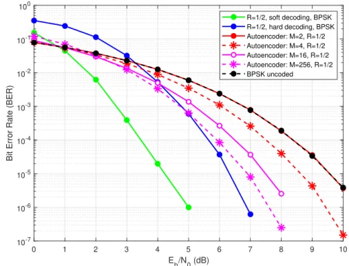
Figures 4.2 - 4.4 show simulated BER performances of different autoencoder models with
R={1/2,1/3,1/4}and their baseline systems with convolutional coding with respective code rates and BPSK modulation scheme. Selected block length for baseline system is
K = 800 and the constraint length of the convolutional encoder/decoder is taken as 7. It can be observed that the BER performance of the autoencoder improves when message size is increasing. For a given code rate, M = 2 model has almost same performance with uncoded BPSK whileM = 256 model has resulted in a much improved BER performance closer to the baseline. This improvement is achieved since the model has more degrees of freedom and more flexibility for a better end-to-end optimization when the message size is high.
0 1 2 3 4 5 6 7 8 9 10 Eb/N0 (dB) 10-7 10-6 10-5 10-4 10-3 10-2 10-1 100
Bit Error Rate (BER)
R=1/2, soft decoding, BPSK R=1/2, hard decoding, BPSK Autoencoder: M=2, R=1/2 Autoencoder: M=4, R=1/2 Autoencoder: M=16, R=1/2 Autoencoder: M=256, R=1/2 BPSK uncoded
Figure 4.2. R = 1/2 system BER performance comparison of different autoencoder models with M ={2,4,16,256}. 0 1 2 3 4 5 6 7 8 9 10 E b/N0 (dB) 10-6 10-5 10-4 10-3 10-2 10-1 100
Bit Error Rate (BER)
R=1/3, soft decoding, BPSK R=1/3, hard decoding, BPSK Autoencoder: M=2, R=1/3 Autoencoder: M=4, R=1/3 Autoencoder: M=16, R=1/3 Autoencoder: M=256, R=1/3 BPSK uncoded
Figure 4.3. R = 1/3 system BER performance comparison of different autoencoder models with M ={2,4,16,256}.
When considering M = 2 and rate R = 1/2 system, number of bits per message is k = log2(2) = 1 and, n = 2 number of channel uses are there to transmit the 1
bit message. For this setup, the best possible signal formulation in each channel use would be to maximize the distance between two message constellation points which is similar to BPSK modulation. Since the autoencoder model dimensions are determined by the parameters M and R, low M values do not result in much coding gain as the non-linearities added by the model during the learning process are limited by the layer dimensions. Increasing the message size increases the layer dimensions and, for a same rateR, the model has more degrees of freedom in terms of learnable parameters which can be optimized to minimize the end-to-end message transmission error. For example, for
M = 256, R= 1/2 system, 16 channel uses are there to transmit 256 different messages which has more flexibility than the earlier scenario where 2 messages are transmitted in 2 channel uses. Thus, when M = 256, R = 1/2, the model has been able to learn the transmit symbols with a channel coding gain as expected, which can be observed from the BER plots. Table 4.2 compares the number of learnable parameters in each layer in above two scenarios which helps us understanding how the model learning capacity increases with increasing message size.
Table 4.2. Learnable parameters R = 1/2 autoencoder models
Layer Number of parameters
(Output dimensions) (M, n) (M=2, n=2) (M=256, n=16) Input (M) 0 0 0 Dense-ReLU (M) (M+1)*M 6 65792 Dense-ReLU (M) (M+1)*M 6 65792 Dense-Linear (2n) (M+1)*2n 12 8224 Normalization (2n) 0 0 0 Noise (2n) 0 0 0 Dense-ReLU (M) (2n+1)*M 10 8448 Dense-ReLU (M) (M+1)*M 6 65792 Dense-Softmax (M) (M+1)*M 6 65792
Even though the autoencoder BER performance is always worse than soft decision CC, it can be observed that autoencoder has a comparable performance to the hard decision CC, specially when the code rate is high. For R = 1/2, autoencoder with M = 256 is better than hard decision CC in lowEb/N0 range from 0 dB to 5 dB and it is only around
0 1 2 3 4 5 6 7 8 9 10 E b/N0 (dB) 10-7 10-6 10-5 10-4 10-3 10-2 10-1 100
Bit Error Rate (BER)
R=1/4, soft decoding, BPSK R=1/4, hard decoding, BPSK Autoencoder: M=2, R=1/4 Autoencoder: M=4, R=1/4 Autoencoder: M=16, R=1/4 Autoencoder: M=256, R=1/4 BPSK uncoded
Figure 4.4. R = 1/4 system BER performance comparison of different autoencoder models with M ={2,4,16,256}.
Figure 4.5 shows the message error rate performances of different autoencoder models with R={1/2,1/3,1/4} and M = 256. We can observe that for the same message size, three models with different rates have resulted in almost same MER, and the models have an acceptable MER performance with a 10−5 error at 7 dB.
0 1 2 3 4 5 6 7 8 Eb/N0 (dB) 10-7 10-6 10-5 10-4 10-3 10-2 10-1 100
Message Error Rate (MER)
Autoencoder: M=256, R=1/2 Autoencoder: M=256, R=1/3 Autoencoder: M=256, R=1/4
Figure 4.5. MER performance of different autoencoder models with R ={1/2,1/3,1/4}
Figures 4.6 and 4.7 compare the autoencoder BER performance for R = {1/2,1/4}
when different block lengths are used in the baseline system with hard decision CC. It can be observed that for R = 1/2 system, baseline BER performance is better for mid-range block lengths where K is 400 - 800 bits. The performance degrades when block size is very low as 200 bits or high as 2000 - 4000 bits, reducing the gap between the autoencoder and baseline BER performance. ForR = 1/4 hard decision CC, there is not much effect on block size for the BER. On the other hand, autoencoder performance is independent of block length K as for a given model with message size M, its input size is k = log2(M) bits where the K bit long block is divided to k bit long sub-blocks and
fed to the system.
Thus, from the results we obtained, autoencoder models would be more effective to be used in high or low input block length scenarios for systems with higher code rates where they have comparable performance to the baseline.
0 1 2 3 4 5 6 7 8 9 10 E b/N0 (dB) 10-7 10-6 10-5 10-4 10-3 10-2 10-1 100
Bit Error Rate (BER)
K=200, R=1/2 hard K=400, R=1/2 hard K=800, R=1/2 hard K=1600, R=1/2 hard K=2000, R=1/2 hard K=4000, R=1/2 hard Autoencoder: M=256, R=1/2 BPSK uncoded
Figure 4.6. R = 1/2 system BER performance comparison for different block lengths: