Decision making with multiple objectives using GAI networks

Decision making with multiple objectives using GAI networks

C. Gonzales, P. Perny

∗

, J.Ph. Dubus

LIP6 – Université Pierre et Marie Curie, case 169, 4 place jussieu, 75005 Paris, France

a r t i c l e

i n f o

a b s t r a c t

Article history:

Received 28 February 2009 Received in revised form 20 July 2010 Accepted 15 September 2010 Available online 2 December 2010 Keywords:

Graphical models GAI decomposable utility Preference representation Multiobjective optimization Multiagent decision making Compromise search Fairness

This paper deals with preference representation on combinatorial domains and preference-based recommendation in the context of multicriteria or multiagent decision making. The alternatives of the decision problem are seen as elements of a product set of attributes and preferences over solutions are represented by generalized additive decomposable (GAI) utility functions modeling individual preferences or criteria. Thanks to decomposability, utility vectors attached to solutions can be compiled into a graphical structure closely related to junction trees, the so-called GAI network. Using this structure, we present preference-based search algorithms for multicriteria or multiagent decision making. Although such models are often non-decomposable over attributes, we actually show that GAI networks are still useful to determine the most preferred alternatives provided preferences are compatible with Pareto dominance. We first present two algorithms for the determination of Pareto-optimal elements. Then the second of these algorithms is adapted so as to directly focus on the preferred solutions. We also provide results of numerical tests showing the practical efficiency of our procedures in various contexts such as compromise search and fair optimization in multicriteria or multiagent problems.

©2010 Elsevier B.V. All rights reserved.

1. Introduction

The complexity of decision problems in organizations, the importance of the issues raised and the increasing need to explain or justify any decision has led decision makers to seek a scientific support in the preparation of their decisions. For many years, rational decision making was understood as solving a single-objective optimization problem, the optimal deci-sion being implicitly defined as a feasible solution minimizing a cost function under some technical constraints. However, the practice of decision making in organizations has shown the limits of such formulations. First, there is some diversity and subjectivity in human preferences that requires distinguishing between the objective description of the alternatives of a choice problem and their value as perceived by individuals. In decision theory, alternatives are often seen as multiattribute items characterized by a tuple in a product set of attributes domains, the preferences of each individual being encoded by a utility function defined on the multiattribute space measuring the relative attractiveness of each tuple. Hence the objectives of individuals take the form of multiattribute utility functions to be maximized. Typically, in a multiagent decision problem, we have to deal with several such utility functions that must be optimized simultaneously. Since individual utilities are gen-erally not commensurate, constructing an overall utility function gathering all relevant aspects is not always possible. Hence the problem does not reduce to a classical single-objective optimization task; we have to solve a multiobjective problem.

Moreover, even when there is a single decision maker, several points of views may be considered in the preference analysis, leading to the definition of several criteria. Rationality in decision making is generally not only a matter of costs reduction. In practice, other significant aspects that are not reducible to costs must be included in the analysis; the outcomes

*

Corresponding author.

E-mail addresses:[email protected](C. Gonzales),[email protected](P. Perny),[email protected](J.Ph. Dubus). 0004-3702/$ – see front matter ©2010 Elsevier B.V. All rights reserved.

of alternatives must be thought in a multidimensional space. This is the case in the elaboration of public policies where different aspects such as ecology and environment, education, health, security, public acceptability are considered in the evaluation process. This is also the case for individual decision of consumers. For example, when choosing a new car for a family, an individual will look at the cost, but will also consider several multiattribute utility functions concerning security in the car (brake system, airbags, . . . ), velocity (speed, acceleration, . . . ), space (boot size, . . . ), environmental aspects (pollution) and aesthetics (color, shape, brand, . . . ). All these observations have motivated the emergence of multicriteria methodologies for preference modeling and human decision support [1–4], an entire stream of research that steadily developed for forty years.

As for human decision making, automated decision making in complex environment requires optimization procedures involving multiple objectives. This is the case when computers are used for planning actions of autonomous agents or for or-ganizing the workflow in production chains. Various other examples can be mentioned such as web search [5],e-commerce and resource allocation problems. In many of them, however, a decision is actually characterized by a combination of lo-cal decisions, thus providing the set of alternatives with a combinatorial structure. This explains the growing interest for multiobjective combinatorial optimization. Besides the explicit introduction of several possibly conflicting objectives in the evaluation process, the necessity of exploring large size solution spaces is an additional source of complexity. This has motivated the development in the AI community of preference representation languages aiming at simplifying preference handling and decision making on combinatorial domains.

As far as utility functions are concerned, the works on compact representation aim at exploiting preference independence among some attributes so as to decompose the utility of a tuple into a sum of smaller utility factors. Different decomposition models of utilities have been developed to model preferences. The most widely used assumes a special kind of independence among attributes called “mutual preferential independence”. It ensures that preferences are representable by an additively decomposable utility [6,7]. Such decomposability makes both the elicitation process and the query optimizations very fast and simple. However, in practice, preferential independence may fail to hold as it rules out any interaction among attributes. Generalizations have thus been proposed in the literature to significantly increase the descriptive power of additive utilities. Among them, multilinear utilities[2] and GAI (generalized additive independence) decompositions [8,9] allow quite general interactions between attributes [7] while preserving some decomposability. The latter has been used to endow CP nets with utilities (UCP nets) both under uncertainty [10] and under certainty [11]. GAI decomposable utilities can be compiled into graphical structures closely related to junction trees, the so-called GAI networks. They can be exploited to perform classical optimization tasks (e.g. find a tuple with maximal utility) using a simple collect/distribute scheme essentially similar to that used in the Bayes net community or to variable elimination algorithms in CSP [12–15]. In order to extend the use of GAI nets to multiobjective optimization tasks, we investigate the potential of GAI models for representing and solving multiobjective optimization problems.

As soon as multiple criteria or utility functions are considered in the evaluation of a solution, the notion of optimality is not straightforward. Among the various optimality criteria, the concept of Pareto optimality or efficiency is the most widely used. A solution is said to be Pareto-optimal or efficient if it cannot be improved on one criterion without being depreciated on another one. Pareto optimality is natural because it does not require any information about the relative importance of criteria and can be used as a preliminary filter to circumscribe the set of reasonable solutions in multiobjective problems. However, in combinatorial optimization problems, the complete enumeration of Pareto-optimal solutions is often infeasible in practice [16–18]. For this reason, in many real applications, people facing such complexity resort to artificial simplifica-tions of the problem, either by focusing on the most important criterion (as in route planning assistants), or by performing a prior linear aggregation of the criteria to get a single objective version of the problem, or by generating samples of good solutions using heuristics, which in any case does not provide formal guarantees on the quality of the solutions.

In this paper, we assume that each objective is represented by a GAI decomposable utility function defined on the multiattribute space describing items. In Section 2, after recalling basic definitions related to GAI nets, we show how they make it possible to represent vector-valued utility functions in a compact form, thus facilitating preference handling in multiobjective decision-making problems. In Section 3, we present two exact algorithms exploiting the structure of the GAI net for the determination of Pareto-optimal elements. In Section 4 we propose a refinement of the second algorithm aiming at focusing the search on specific compromise solutions within the Pareto set. We provide exact algorithms for preference-based search with various preference models. The potential of this approach is illustrated in the context of fair multiagent optimization or in the context of compromise search in multicriteria optimization. Finally, in Section 5, we present numerical tests showing the practical feasibility of the proposed approach on various instances of multiobjective combinatorial problems.

2. Multidimensional GAI nets

We assume that alternatives are characterized bynattributesx1, . . . ,xn taking their values in finite domains X1, . . . ,Xn

respectively. Hence alternatives can be seen as elements of the product set of these domains

X

=

X1

× · · · ×

Xn. In the

sequel,N

= {

1

, . . . ,

n

}

will denote the set of all the attributes’ indices. By abuse of notation, for any setY

⊆

N, XYwill refer

to the Cartesian product of the Xi,i

∈

Y, i.e., XY

=

i∈YXi, and xY will refer to the projection of x

∈

X

on XY, that is,

the tuple formed by the xi,i

∈

Y. We also consider a binary relation

over

X

(actually this is a weak order). Essentially, x

y means thatx is at least as good as y. Symbol

refers to the asymmetric part of

and

∼

to the symmetric one.

are thus needed. Some generalizations of additive utilities have thus been investigated. For instanceutility independenceon every Xileads to a more sophisticated form called amultilinear utility[7]. Such utilities are more general than additive ones

but still cannot cope with many kinds of interactions among attributes. To increase the descriptive power of such models, GAI (generalized additive independence) decompositions have been introduced by [20], that allow more general interactions between attributes [7,9,8,21] while still preserving some decomposability.

2.1. GAI models and GAI nets

GAI decomposition is a generalization of the additive decomposition in which subutilities ui are allowed to be defined

over overlapping factors. As such, they include additive and multilinear decompositions as special cases. They can be more formally defined as follows:

Definition 1.LetC1, . . . ,Ckbe subsets ofNsuch thatN

=

k

i=1Ci. A utilityu

(

·

)

representing

over

X

is GAI-decomposable

w.r.t. the XCi iff there exist functionsui:XCi

→

Z

+such that:

u(x1

, . . . ,

xn

)

=

k

i=1

ui

(x

Ci

),

for allx

=

(x

1

, . . . ,

xn

)

∈

X

.

Example 1.Utility functionu

(

a

,

b

,

c

,

d

,

e

,

f

,

g

)

=

u1(a

,

b

)

+

u2(b

,

c

,

d

)

+

u3(c

,

e

)

+

u4(b

,

d

,

f

)

+

u5(b

,

g

)

defined on A

×

B

×

C

×

D

×

E

×

F

×

G is a GAI-decomposable utility, with XC1

=

A

×

B, XC2

=

B

×

C

×

D, XC3

=

C

×

E, XC4

=

B

×

D

×

F and XC5

=

B

×

G.

GAI decompositions can be represented by graphical structures we callGAI networks[9,21] which are essentially similar to junction graphs used in the Bayesian network literature [22,23]:

Definition 2.Letu

(

x1, . . . ,xn

)

=

ki=1ui

(

xCi

)

be a GAI utility function over

X

. A GAI network representingu

(

·

)

is an

undi-rected graph

G

=

(

C

,

E

)

satisfying the following three properties:

Property 1:

C

= {

XC1

, . . . ,

XCk

}

. Vertices XCi are calledcliques. To each vertex XCi is associated the corresponding subu-tility factoruifrom the utility functionu;

Property 2:

(

XCi

,

XCj

)

∈

E

⇒

Ci

∩

Cj

= ∅

. Edges

(

XCi

,

XCj

)

are labeled by XSi j, where Si j

=

Ci

∩

Cj. XSi j is called a separator. Separator XSi j thus corresponds to the attributes that the two cliques XCi andXCj have in common;

Property 3: for allXCi

,

XCj such thatCi

∩

Cj

=

Si j

= ∅

, there exists a path between XCi andXCj in

G

such that for every clique XCh in this path Si j

⊆

Ch (running intersection property).

In the rest of the paper, theXCi will always denote cliques of a GAI network and the XSi j will always denote the separator, i.e., the intersection, between cliquesXCi andXCj. By abuse of notation, XSii will refer to clique XCi itself. Cliques are usually drawn as ellipses and separators as rectangles. For any GAI decomposition, by Definition 2, the cliques of the GAI network should be the sets of attributes of the subutilities. The edges in the network represent the intersections between subsets of attributes. As the intersections are commutative, the GAI network is an undirected graph. Note that this contrasts with UCP nets, where the relationships between vertices in the network correspond to conditional dependencies, thus justifying the use of directed graphs for UCP nets. For any clique XCi, Adj

(

XCi

)

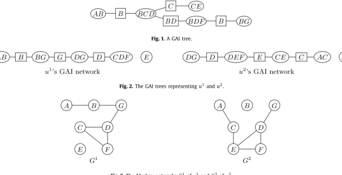
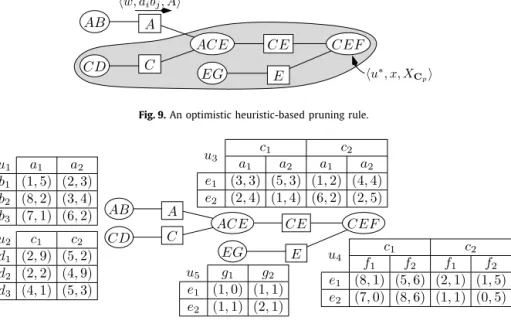
will refer to the set of cliques adjacent to XCi.

In this paper, we shall only be interested in GAI trees. As we shall see, this is not restrictive as general GAI networks can always be compiled into GAI trees. The set of edges of a GAI network can be determined by any algorithm preserving the running intersection property (see the Bayesian network literature on this matter [23]). Fig. 1 shows one possible GAI network representing the GAI utility of Example 1. Note that this network is not the unique representation of the utility function.

Fig. 1.A GAI tree.

Fig. 2.The GAI trees representingu1_andu2_.

Fig. 3.The Markov networksG1_ofu1_andG2_ofu2_. 2.2. Handling multiple objectives

Consider now a finite set of objectives M

= {

1

, . . . ,

m

}

and assume that any solution x

∈

X

is characterized by a utility vector

(

u1

₍

_x

_{), . . . ,}

_um

₍

_x

₎₎

_∈

_Z

m

+ whereui:

X

→

Z

+ is theith utility function. This function measures the relative utility of alternatives with respect to the ith point of view (criterion or agent) considered in the problem. Hence, the comparison of alternatives reduces to that of their utility vectors, i.e., instead of comparing alternatives xand y through the numbers assigned to them by utilityuas in the preceding subsection, we now compare them through vectors

(

u1

₍

_x

_{), . . . ,}

_um

₍

_x

₎₎

_and

(

u1

(

y

), . . . ,

um

(

y

))

.

The ui _{are functions}

_X

_→

_Z

+. Hence, separately, they can be considered as single utility functions. Assuming that each objective corresponds to a given agent, each ui _{corresponds to the utility function representing the agent’s preferences and}

vectors

(

u1

(

x

), . . . ,

um

(

x

))

correspond to the utility of the group of agents. Now, if a ui is the utility function of a given agent, by the preceding subsection, it may be GAI decomposable. Thus, assume that all theui_{are decomposable according}

to the same GAI net given in Fig. 1. Then, for any i

∈

M,

ui

(a,

b,c,d,e,f

,

g)

=

ui₁

(a,b)

+

ui₂

(b,c,d)

+

ui₃

(c,e)

+

u₄i

(b,d,

f

)

+

ui₅

(b,

g).

Note that, even if the values of the ui_j differ from one agent to another, all these utilities can be stored in the GAI net of Fig. 1 as follows: store all functions ui₁,i

∈

M, in clique A B, store all functionsui₂,i

∈

M, in clique BC D, and so on. Hence the GAI networks described in Section 2.1 can be easily adapted to the multiobjective case. The key property that enables this generalization to the multiobjective case is the fact that all the subutilitiesui

j are defined on attribute sets (here XCj) included in at least one clique of the GAI net. For instance, theui₁are defined on A

×

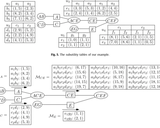
Band can thus be stored in any clique containing both attributes AandB (here cliqueA Bis the only possible choice).

Let us now consider the case where the agents have preferences that are not decomposable according to the same GAI network. For simplicity, we will illustrate our point for the two agent/objective case:m

=

2. So suppose thatu1_andu2 _can be decomposed as follows:

u1

(a,b,

c,d,e,f

,

g)

=

u1₁

(a,

b)

+

u1₂

(b,

g)

+

u1₃

(d,

g)

+

u1₄

(c,

d,f

)

+

u1₅

(e),

u2

(a,b,

c,d,e,f

,

g)

=

u2₁

(a,

c)

+

u2₂

(b)

+

u2₃

(d,

g)

+

u2₄

(d,e,

f

)

+

u2₅

(c,e).

(1)

These decompositions correspond to the GAI networks of Fig. 2. Note that none of these trees can be used to store both u1 andu2, the left graph being unable to store u2₄

(

d

,

e

,

f

)

, and the right one being unable to storeu1₁

(

a

,

b

)

. We thus need to construct another GAI tree that can contain both u1 and u2. To construct this new GAI network, we will first create another graph per ui_{, called a Markov network. In this graph, each node corresponds to an attribute X}

i, and two nodes Xi

,

Xj are connected by an edge if and only if there exists a subutilityuh:XCh

→

Z

+ such thati

,

j

∈

Ch. In other words, the set of attributes over whichuhis defined contains both Xiand Xj. Hence, in the Markov network, to each subutilityuh

corresponds a clique (a complete subgraph). Fig. 3 displays the Markov networks ofu1andu2 as described in Eq. (1). Now, create the union of both graphs, i.e., the Markov network containing an edge between two nodes if and only if G1 _{and/or G}2 _{contains the same edge. The union of G}1 _andG2 _{is represented in Fig. 4(a). Next, this graph is triangulated}

using any triangulation technique [24–26]. Finally, the triangulated graph is mapped into a GAI network: each maximal complete subgraph corresponds to a clique of the GAI network. In the latter, edges are added by any algorithm preserving the running intersection property [23]. In [27], Rose guarantees that whenever the cliques of a GAI net correspond to the maximal complete subgraphs of a triangulated Markov network, then the GAI net is a tree.

Hence, given a set u1

, . . . ,

um of utilities, each one having its own GAI decomposition over

X

, a global GAI tree can be constructed to store all these utilities. In the sequel, instead of storingm utilitiesui_j:XCj

→

Z

+,i

∈ {

1

, . . . ,

m

}

, in each clique XCj, we chose an alternative but equivalent representation: we just store one vector-valued utilityuj:XCj

→

Z

m +such thatuj

(

xCj

)

=

(

u 1 j

(

xCj

), . . . ,

u m j

(

xCj

))

. 3. Pareto search 3.1. Problem formulation

The set of all utility vectors attached to solutions in

X

is denoted by

U

. We recall now some definitions related to dominance and optimality in multiobjective optimization.

Definition 3.The weak Pareto dominance relation is defined on utility vectors of

Z

m

+as:u

Pv

⇔ [∀

i

∈

M

,

ui

vi

]

.

Definition 4. The Pareto dominance relation

P is defined as the asymmetric part of

P: u

P v

⇔ [

u

P v and

not

(

v

Pu

)

]

.

Definition 5.Any utility vectoru

∈

U

is said to be non-dominated in

U

(or Pareto-optimal) if

v

∈

U

such that v

Pu. The

set of non-dominated vectors in

U

is denotedND

(

U

)

and is referred to as the “Pareto set”. The problem of determining the Pareto set in

X

can be stated as follows:

Pareto-optimal elements (PO)

Input: a product set of finite domains

X

=

X1

×· · ·×

Xn(nfinite),mGAI utility functionsui:

X

→

Z

+

,

i

=

1

, . . . ,

m(mfinite), Goal: determine the entire set of non-dominated vectors in

U

, and for each utility vectoru

∈

ND

(

U

)

a corresponding tuple xu

∈

X

.

This problem is generally intractable on large size instances. Even whenm

=

2, it may happen that the size of the Pareto set grows exponentially with the number of attributes, as shown by the following example:

Example 2.Consider an instance of PO with two objectives

(

m

=

2

)

on a set

X

=

n_j=1Xj, where Xj

= {

0

,

1

}

, j

=

1

, . . . ,

n.

Assume that the objectives are additive utility functions defined, for any Boolean vector x

=

(

x1, . . . ,xn

)

∈

X

, byui

(

x

)

=

n

j=1uij

(

xj

)

,i

=

1

,

2

,

whereu i

jis a marginal utility function defined on Xj by u 1

j

(

xj

)

=

2 j−1_x

j andu2_j

(

xj

)

=

2j−1

(

1

−

xj

)

.

Then for all x

∈ {

0

,

1

}

n_{, u}1

₍

_x

₎

₌

n

j=12j−1xj andu2

(

x

)

=

nj=12j−1

(

1

−

xj

)

and therefore u1

(

x

)

+

u2

(

x

)

=

nj=12j−1

=

2n

₋

_{1. So there exists 2}n _{different Boolean vectors in}

_X

_{, with distinct images in the utility space, all being located on the}

same line characterized by equationu1

+

u2

=

2n

−

1. This line is orthogonal to vector

(

1

,

1

)

which proves that all these vectors are Pareto-optimal. HereND

(

U

)

=

U

.

Although pathological, this example shows that the determination of the entire Pareto set may induce prohibitive run times in practice on large size instances with two criteria or more. Numerical tests presented in Section 5 will confirm this point. We establish now a complexity result concerning problem PO (proofs are given in Appendix A).

Proposition 1.As soon as

|

Xi

|

2

,

i

∈

N, and m

2, deciding whether there exists a tuple in

X

the utility vector of which weakly

3.2. Multiobjective optimization algorithms

Despite the worst case complexity of problem PO, we may expect to solve real instances of reasonable size in admissible times. To this end, we introduce below solution algorithms for PO based on message propagation schemes within the GAI network. For clarity reasons, we first present a variable elimination PO algorithm that processes all the vectors of a given clique before removing it from the GAI network. In the next subsections, we will consider best-first variations of this algorithm which will be more efficient for preference-based search.

3.2.1. A variable elimination algorithm

The algorithm described below is a direct application of variable elimination to determine the Pareto set. Its principle has already been used for CSP in [28]. The algorithm extensively relies on the following proposition and its corollaries:

Proposition 2.Let

(

D

,

E

)

be a partition ofN. Assume that utility u:

X

→

Z

m₊ is additively decomposable as u

=

u1

+

u2, with

u1:XD

→

Z

m₊and u2:XE

→

Z

m₊(here,

+

unambiguously refers to the pointwise addition over vectors). Then:

ND(

U

)

⊆

ND

u1

(x

D

),

xD

∈

XD

ND

u2

(x

E

),

xE

∈

XE

,

(2)

where, for any sets

V

,

W

of vectors of

Z

m₊,

V

W

is defined as

V

W

= {

v

+

w

,

v

∈

V

,

w

∈

W}

.

In other words, undominated utility vectors of

U

can only result from the addition of one undominated utility vector from subset XD and one undominated utility vector from subset XE. For instance, if u:A

×

B

→

Z

+ is decomposable as u1(A

)

+

u2(B

)

whereu1 andu2 are defined as:

u1

=

a1 a2 a3

(

3

,

4

) (

4

,

2

) (

2

,

3

)

u2

=

b1 b2 b3

(

3

,

5

) (

6

,

3

) (

3

,

3

)

ThenND

(

{

u1(ai

)

}

)

= {

u1(a1)

=

(

3

,

4

),

u1(a2)

=

(

4

,

2

)

}

andND

(

{

u2(bi

)

}

)

= {

u2(b1)

=

(

3

,

5

),

u2(b2)

=

(

6

,

3

)

}

which, composed

with operator

, produce the following set:

u(a1

,

b1

)

=

(

6

,

9

),

u(a1

,b

2

)

=

(

9

,

7

),

u(a2

,b

1

)

=

(

7

,

7

),

u(a2

,

b2

)

=

(

10

,

5

)

.

Therefore ND

(

U

)

= {

u

(

a1,b1),u

(

a1,b2),u

(

a2,b2)

}

. Note that no Pareto element involvesu1(a3)oru2(b3), which are domi-nated inND

(

{

u1(ai

)

}

)

andND

(

{

u2(bi

)

}

)

respectively.

As a consequence, ifu is additively decomposable, an efficient procedure to determineND

(

U

)

can be to first determine independently ND

(

{

u

(

xD

),

xD

∈

XD}

)

and ND

(

{

u

(

xE

),

xE

∈

XE}

)

, then sum-up all these vectors, and finally keep only the

undominated resulting vectors.

Corollary 1.Let

G

be a GAI tree with only two cliques XC1and XC2and their separator XS12. LetD1

=

C1

\

S12andD2

=

C2

\

S12, i.e., the

Diare the indices of the attributes that appear inCibut not inC3−i(or in other words, they appear only on one side of the separator). Then: ND(

U

)

⊆

xS₁₂∈XS₁₂

ND

u1

(x

D1

,x

S12

),

xD1

∈

XD1

ND

u2

(x

D2

,

xS12

),

xD2

∈

XD2

.

In other words, for each fixed value xS12 of XS12, if a utility vectoru1(yD1

,

xS12

)

is Pareto dominated by another vector u1(xD1

,

xS12

)

defined for the same value of the separator, no combination ofu1(yD1

,

xS12

)

with another vectoru2(xD2

,

xS12

)

can result in a vector of ND

(

U

)

. Hence, to determineND

(

U

)

, first determine the undominated vectors of typeu1(xD1

,

xS12

)

andu2(xD2

,

xS12

)

and sum them up for any fixed valuexS12, then keep only those that are undominated.

Corollary 2.Let

G

=

(

C

,

E

)

be any GAI network, with

C

= {

XC1

, . . . ,

XCk

}

, and let XSi j be any separator. Let

{

XCi1

, . . . ,

XCir

}

and

{

XC_ir+1

, . . . ,

XC_ik

}

be the sets of cliques on each side of separator XSi jand letD

=

r t=1Cit

\

Si jandE

=

k t=r+1Cit

\

Si j. Then: ND(

U

)

⊆

xS_{i j}∈XS_{i j}

ND

_r

t=1 ut

(x

C_it

),

xD

∈

XD

ND

_k

t=r+1 ut

(x

C_it

),

xE

∈

XE

.

In other words, to determine ND

(

U

)

, it is sufficient to select any separator, then compute for each fixed value xSi j of this separator the undominated utility vectors on each side of the separator and sum-up all these vectors. Finally gather all these vectors for all the values xSi j and keep only the undominated ones.

Corollary 2 can now be exploited recursively to compute the Pareto set over

U

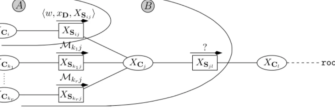
: consider the GAI network of Fig. 5, in which subutility tables are displayed next to their corresponding clique. The overall utility function u over A

×

B

×

C

×

D

×

E

×

F

×

G is thus decomposable as:u1(A

,

B

)

+

u2(C

,

D

)

+

u3(A

,

C

,

E

)

+

u4(C

,

E

,

F

)

+

u5(E

,

G

)

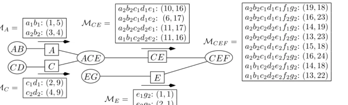
. Using Corollary 2

Fig. 5.The subutility tables of our example.

Fig. 6.The messagesMi.

with separator A, we can conclude that vectors in ND

(

U

)

can only result from the sum of vectors u2,u3, . . . , to vectors u1(A

,

B

)

that are undominatedfor fixed values of A. Send the latter as message

M

Aon separator A (see Fig. 6). Similarly,

by Corollary 2 with separator C (resp. E), only vectors u2(C

,

D

)

(resp. u5(E

,

G

)

) that are undominated for fixed values of C (resp. E) can lead to vectors in ND

(

U

)

. Send these vectors as message

M

C on separator C and message

M

E on

separator E respectively. Now, apply Corollary 2 with separator C E: vectors in ND

(

U

)

can only derive from undominated vectorsu1

+

u2

+

u3 for fixed values ofC E. But we already know that vectorsu1 (resp.u2) that are dominated for fixed values ofA (resp.C) cannot be part of a vector inND

(

U

)

. As a consequence, the undominated vectorsu1

+

u2

+

u3for fixed values ofC E can be determined by first computing all the possible vectorsu1

+

u2

+

u3 with vectorsu1 andu2 restricted to

M

A and

M

C respectively, and, then, keeping for each value of C E the undominated ones. In other words, we should

compute

M

C E

(

c

,

e

)

=

ND

(

a∈A

M

A

(

a

)

{

u2(a

,

c

,

e

)

}

M

C

(

c

))

for everyc

,

e

∈

C

×

E. This results in an overall separator’s

message

M

C E

= {M

C E

(

c

,

e

)

: c

,

e

∈

C

×

E

}

. Now there just remains to combine the vectors of

M

C E,

M

E andu4(C

,

E

,

F

)

and keep the undominated ones: these are the Pareto set ND

(

U

)

=

ND

(

_{c,e,f∈C×E×F}

M

C E

(

c

,

e

)

u4(c

,

e

,

f

)

M

E

(

e

))

.

Indeed, this combination corresponds to the combination of all the possible vectorsui except those that are known not to

be part ofND

(

U

)

. In the end,ND

(

U

)

= {

u

(

a1b1c1d1e2f2g2)

=

(

15

,

25

)

;

u

(

a1b2c1d1e2f2g2)

=

(

22

,

22

)

;

u

(

a1b2c1d2e2f2g2)

=

(

24

,

14

)

;

u

(

a2b2c1d1e2f2g2)

=

(

16

,

24

)

}

.

Note the gain resulting from the application of Corollary 2: for instance, for computing message

M

C E, we needed only

40 additions (16 additions to compute

M

A

M

C, out of which 4 vectors were removed because they were dominated,

and then 24 additions to combine the 12 remaining vectors withu3) instead of 72 additions if we had computedu1

+

u2

+

u3 over A

×

B

×

C

×

D

×

E. Similarly, computing ND

(

U

)

=

ND

(

c,e,f∈C×E×F

M

C E

(

c

,

e

)

u4(c

,

e

,

f

)

M

E

(

e

))

required 8

additions to computeu4(c

,

e

,

f

)

M

E

(

e

)

, and then 30 additions to compute the addition of the result with message

M

C E.

Overall, we computed 78 additions instead of the 298 needed if we had computedu over the whole Cartesian product

X

. The procedure described above justifies a “collect” algorithm where a clique (here C E F) collects all the information from its neighbors (via messages

M

i) to compute the Pareto set. To produce these messages the neighbors also collect the

necessary information from their other neighbors, and so on. This results in function

Pareto

described below. However, to define this algorithm and the next ones more conveniently, we will not work directly with subutility vectors as we did above but rather with labels:

Definition 6.A label is a triple

v

,

xC

,

XSi j

, where vis a vector of

Z

m

+,xC

∈

XC is an instantiation of a set XC of attributes,

Intuitively, a label

v

,

xC

,

XSi j

corresponds to subutility vectorv, with the additional information of the partial instanti-ation xC of the attributes that were involved in its construction and the separator XSi j on which the message containing v has been transmitted. Given a clique XCi the subutility of which isui:XCi

→

Z

m

+, we define the set of labels corresponding

to ui asLabels

(

XCi

)

= {

ui

(

xCi

),

xCi

,

XCi

: xCi

∈

XCi

}

. In addition, to handle labels easily, we define for any set of labels

V

,

W

, any set of attributes XE and any instantiationxE

∈

XE, the following operators:

•

ND

(

V

)

denotes a set of labels of

V

the utility vectors of which are undominated (actually, we keep inND

(

V

)

only one label per undominated vector, that is, we are interested only in one instantiation for each utility vector).

•

V

⊗

W

= {

v

+

w

,

xC∪D

,

XE∪F:

v

,

xC

,

XE ∈

V

and

w

,

xD

,

XF ∈

W}

, i.e., operator

⊗

aggregates additively labels of

V

and

W

the partial instantiations of which agree on attributes XC∩D. This operator will be used extensively to combine

appropriately the aforementioned messages.

•

V

→XE

= {

v

,

xD

,

XE

:

v

,

xD

,

XF ∈

V}

, i.e.,

V

→XE contains the same labels as

V

except that their third component is

substituted by XE. This will be used to “move” messages from one separator to another one.

•

V[

xE] = {v

,

yD

,

XF ∈

V

: yE

=

xE

}

, i.e.,

V[

xE]is the subset of labels of

V

that “agree” with partial instantiation xE.

•

V

⇓X_E

=

xE∈XEND

(

V[

xE]

)

→XE, i.e.,

V

⇓X_E contains the set of all the labels of

V

that are undominated by any other label of

V

with the same partial instantiation xE. This operator will be used to discard all the labels the combination of

which cannot lead to undominated solutions due to Corollary 2.

Given these operators, we can now express the basic message-passing algorithm we described above for computing the Pareto set1:

Algorithm 1: A variable elimination algorithm for computing the Pareto set.

FunctionPareto_Collect(XCi,XCj)

01 messageMi j←Labels(XCi)

02for allcliquesXCk∈Adj(XCi)\{XCj}do FunctionPareto( )

03 callPareto_Collect(XCk,XCi) 01 Letroot=XCpbe any clique

04 Mi j←Mi j⊗Mki 02 callPareto_Collect(XCp,XCp)

05done 03 returnND(Mpp) 06Mi j←Mi j_⇓X

Si j

Proposition 3.Given a GAI tree

G

, function

Pareto

()

returns precisely the Pareto set.

Proposition 4.(See Rollon and Larrosa [28].)

Pareto

()

requires space O

(

km

×

m_i=1Ki

×

dw

∗

)

and time O

(

km

×

m_i=1K2 i

×

dw

∗₊₁

)

, where k is the number of cliques in the GAI network, d is the largest attribute’s domain size, w∗is the network’s induced width(i.e., the number of variables in the largest clique minus one)and Kiis a bound on utility ui.

Note that function

Pareto_Collect, as described above, is generic and does not impose any ordering on messages

M

ki’s combinations. In practice, the number of operations performed during the

for

loop of lines 02–05 depends on how

combinations are performed. A simple yet very effective strategy consists in, first, computing all the

M

ki by calling the

appropriate

Pareto_Collect

(

XCk

,

XCi

)

and, only then, perform the combinations. The latter can be computed iteratively by always selecting the pair of messages that produces a message with the smallest dimension. For instance, assume that we wish to compute

M

1i

⊗

M

2i

⊗

M

3i, with messages

M

1i,

M

2i,

M

3i defined on A

×

B,A

×

C andC

×

D respectively.

Then first computing

M

1

=

M

1i

⊗

M

2i, and then

M

1

⊗

M

3iproduces the same result as computing

M

2

=

M

1i

⊗

M

3i,

and then

M

2

⊗

M

2ibut the former is faster than the latter since

M

1 is defined onA

×

B

×

C whereas

M

2is defined on A

×

B

×

C

×

D.

3.2.2. A best-first Pareto search algorithm

In function

Pareto

()

described previously, sending all the subutility vectors that are undominated for fixed separator values in one single message

M

i j prevents applying prunings that can significantly speed-up the algorithm. For this reason,

we now propose an alternative algorithm that sends the undominated subutility vectors (labels actually) one by one on the separators. When such vector reaches the

root

clique, this vector produces new knowledge that can be used to prune those vectors that have not reached the

root

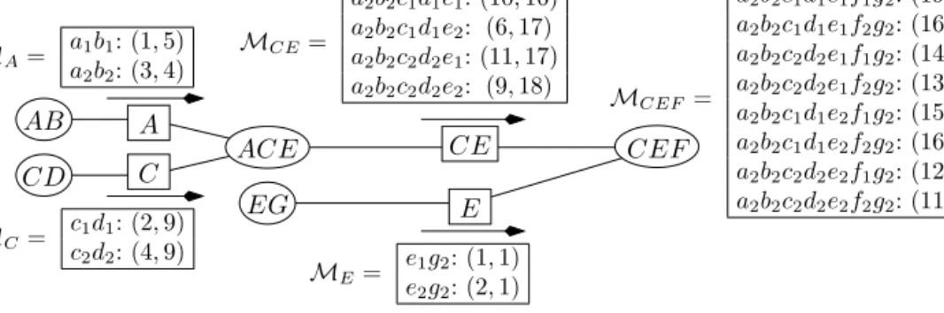
yet and that we now know for sure cannot be part of the solution. This algorithm is very similar in spirit to the variant of the MOA∗ algorithm by Mandow and de la Cruz [29] that improves the standardMOA∗algorithm [30–32]. It favors the early detection of partial solutions that will lead to suboptimal solutions and can therefore discard the corresponding labels hence limiting the combinatorial blowup. The main difference between our approach and MOA∗ lies in the exploitation of an explicit junction tree structure instead of an implicit state space graph.

1 _{Recall that, by abuse of notation,X}

Fig. 7.Making a label move towardroot.

On one hand, our search algorithm requires satisfying specific constraints imposed by the junction tree. Actually, whenever a label is moved from one separator to the next one, it is combined with other labels stored into adjacent separators; to ensure that this combination is meaningful, the partial instantiations of these labels must necessarily be compatible. Thus, our approach needs more information about how labels were generated than MOA∗ usually does. On the other hand, as our best-first search algorithm is based on the tree structure of the GAI network and proceeds from leaves toward the

root

clique, a given label can never be generated more than once. Thus, unlikeMOA∗, our algorithm does not need to keep track of a list ofclosedlabels and, actually, it never stores such a list. In a sense, this feature is close tofrontier search algorithms [33].

More precisely, the idea is to maintain two lists of labels:

L

open, which are the labels that have not reached yet the

root

clique, and

L

Pareto, which are essentially those labels that have reached

root

and are still undominated. At the beginning of the algorithm,

L

Pareto_{should be empty, and}

_L

open_{should be basically filled with the labels of the leaves of the GAI network.}

A nonempty

L

open _{set means that there still exist labels that can possibly be combined with other labels to produce in}

the end undominated labels that should belong to

L

Pareto. So, while

L

openis nonempty, select one of its labels and make it move toward

root

(by combining it with other appropriate labels, see below). When a label reaches

root, it is of course

discarded from

L

open_and

_L

Pareto_{is updated. When all the labels of interest have reached}

_{root, then}

_L

open_{becomes empty}

and the algorithm has computed the Pareto set.

To illustrate how labels move toward the root, consider an arbitrary label

w

,

xD

,

XSi j

which is currently located on separator XSi j (see Fig. 7). Like in function

Pareto

()

, this label corresponds to the subutility of a partial instantiation of the attributes in the “A” area of the GAI net. Moving it to separator XSjl should thus logically produce a label corresponding to the instantiation of the attributes in the “B” area of the GAI net. Hence

w

,

xD

,

XSi j

should necessarily be added to compatible labels located on separators XSk1j

, . . . ,

XSkr j as well as to compatible labels stored in clique XCj (else some attributes in the “B” area would remain uninstantiated). Among all such possible labels, those that were sent on separators XSk1j

, . . . ,

XSkr j at earlier steps of the algorithm seem to be good candidates. So let us consider the set of labels

M

ktj, t

=

1

, . . . ,

r, sent on these separators at earlier steps. We propose to generate all the compatible combinations of these messages, i.e.,

{

w

,

xD

,

XSi j

} ⊗

M

k1j

⊗ · · · ⊗

M

krj

⊗

Labels

(

XCj

)

, and then to project the resulting set of labels on separator XSjl (discarding of course all the dominated labels for fixed values ofXSjl) or, in other words, to compute:

V

=

w,xD

,

XSi j

⊗

M

k1j

⊗ · · · ⊗

M

krj

⊗

Labels(XCj

)

_⇓X

S_jl

.

(3)

The labels in

V

thus correspond to a set of labels appropriate for separator XSjl. As such they should be added to

L

open _since

_L

open _{represents the sets of labels that may potentially be part of the Pareto solutions we look for. In}

addi-tion, label

w

,

xD

,

XSi j

can now be safely removed from

L

open _{since it has been dealt with (i.e., it has been combined}

with other labels). The process just described informally can now be described algorithmically by the following func-tion:

Algorithm 2: The function for moving labels within the Junction tree.

Functionmove_label(w,xD,XSi j)

01Mi j←Mi j∪ {w,xD,XSi j}

02V←Labels(XCj)⊗ {w,xD,XSi j}

03ifXCj=rootthenletXClbe the clique∈Adj(XCj)s.t.XClis on the path betweenXCjandroot

04for allcliquesXCk∈Adj(XCj),XCk=XCiandXCk=XCl(ifXClhas been defined in line 02)do

05 V←V⊗Mkj 06done

07ifXCj=rootthenV←V⇓XSjl elseV←ND(V)

Of course, Eq. (3) produces a set of labels corresponding to instantiations of all the attributes of the “B” area of Fig. 7 if and only if all messages

M

ktj are nonempty. Hence we should enforce that whenever function

move_label

is called, the

M

ktj are actually nonempty. A simple way to achieve this is to initialize the Pareto search by function

ini-tial_labels

below which fills each separator XSi j with exactly one label per valuexSi j. The basic idea of the function is to apply a collect scheme from

root

toward the leaves of the GAI tree and, each time a separator is encountered, to fill it with one label per value. More precisely, for separators on the leaves of the tree, we compute the set of undom-inated labels per value of the separator, say

V

_⇓X

S_{i j}. As this set may contain several labels per value xSi j, we just keep one label per xSi j (this produces a message

M

i j) and put the other ones into

L

open _{to be processed later on. When}

we encounter a separator XSjl like in Fig. 7, the collect scheme first fills separators XSi j

,

XSk1j

, . . . ,

XSkr j with messages

MS

i j

,

MS

k1j

, . . . ,

MS

kr j respectively. Now, these messages can be combined to produce a message that can be stored on XSjl:

V

=

(

MS

i j

⊗

MS

k₁j

⊗ · · · ⊗

MS

kr j

⊗

Labels

(

XCj

))

_⇓

X_S jl

. Again,

V

may contain several messages per valuexSjl, hence we store only one of them into message

M

jl and put the other ones into

L

opento be processed later on. Of course, as the label

chosen to be stored into

M

jl is processed immediately while the others (those added to

L

open) will be processed later,

the former should be selected as the one that currently seems best fitted to produce a Pareto element when moved till the

root. For this reason, we call this element a “

most promising” label. Different strategies do exist to define what a most promising label should be. In our experiments, we defined it as being the label with the highest utility average (over theM objectives). When optimistic heuristics were available, we used the highest average of the sum of the utility vector and the heuristic vector. Of course, alternative characterizations could also have been used such as, e.g., the highest lexicographic utility value (using a lexicographic order over the objectives). Overall, the above algorithm leads to the following function

initial_labels:

Algorithm 3: The function initializing separator messages with one label per separator’s value.

Functioninitial_labels(XCi,XCj)

01V←Labels(XCi)

02for allcliquesXCk∈Adj(XCi)\{XCj}do

03 callinitial_labels(XCk,XCi)

04 V←V⊗Mki 05done

06V←V⇓XSi j

07Mi j=xSi j∈XSi j most promising label ofV[xSi j]

08Lopen_←Lopen_∪(V\M i j)

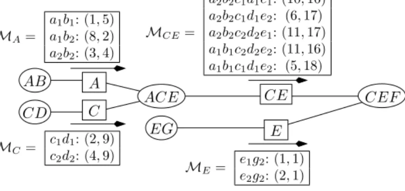
Let us illustrate this algorithm on the GAI net of Fig. 5: a call to

initial_labels

(

C E F

,

C E F

)

would call

initial_labels

(

E G

,

C E F

)

and

initial_labels

(

AC E

,

C E F

)

on line 03. The first call first creates set

V

= {

(

1

,

0

),

e1g1,E G

,

(

1

,

1

),

e1g2,E G

,

(

1

,

1

),

e2g1,E G

,

(

2

,

1

),

e2g2,E G

}

on line 01 and

V

is reduced to

V

= {

(

1

,

1

),

e1g2,E

,

(

2

,

1

),

e2g2,E

}

on line 06. As

V

contains only one label per separator’s value e1,e2, message

M

E

=

V

as shown in

Fig. 8. Now

initial_labels

(

AC E

,

C E F

)

calls

initial_labels

(

A B

,

AC E

)

and

initial_labels

(

C D

,

AC E

)

. The first one will compute

V

= {

(

1

,

5

),

a1b1,A

,

(

8

,

2

),

a1b2,A

,

(

3

,

4

),

a2b2,A

,

(

6

,

2

),

a2b3,A

}

on line 06 (discarding both labels

(

7

,

1

),

a1b3,A

and

(

2

,

3

),

a2b1,A

because they are dominated by

(

8

,

2

),

a1b2,A

and

(

3

,

4

),

a2b2,A

respectively). Here,

V

contains more than one element perai, so we need select only one element peraiin

V

to create message

M

A. Say

M

A

=

{

(

1

,

5

),

a1b1,A

,

(

3

,

4

),

a2b2,A

}

(see Fig. 8). Note that, in this example, to reduce the number of iterations of the algorithm, the most promising label is not always chosen as the one with the highest utility average. The other elements of

V

, i.e.,

{

(

8

,

2

),

a1b2,A

,

(

6

,

2

),

a2b3,A

}

are thus added to

L

open to be processed later on. Similarly,

initial_labels

(

C D

,

AC E

)

computes on line 06 label set

V

= {

(

2

,

9

),

c1d1,C

,

(

4

,

1

),

c1d3,C

,

(

4

,

9

),

c2d2,C

,

(

5

,

3

),

c2d3,C

}

. From

V

we extract message

M

C

= {

(

2

,

9

),

c1d1,C

,

(

4

,

9

),

c2d2,C

}

and labels

(

4

,

1

),

c1d3,C

and

(

5

,

3

),

c2d3,C

are added to

L

open to be processed later on. Now

initial_labels

(

AC E

,

C E F

)

can compute label set

[

Labels

(

AC E

)

⊗

M

A

⊗

M

C

]

_⇓C E, which leads to:

V

=

(

6

,

17

),

a1b1c1d1e1

,

C E

,

(

10

,

16

),a

2b2c1d1e1

,

C E

,

(

5

,

18

),

a1b1c1d1e2

,

C E

,

(

6

,

17

),

a2b2c1d1e2

,

C E

,

(

11

,

17

),a

2b2c2d2e1

,

C E

,

(

9

,

18

),

a2b2c2d2e2

,

C E

on line 06. From this set, we extract message

M

C E by selecting one label per value

(

ci

,

ej

)

:

M

C E

=

(

10

,

16

),

a2b2c1d1e1

,

C E

,

(

6

,

17

),a

2b2c1d1e2

,

C E

,

(

11

,

17

),

a2b2c2d2e1

,

C E

,

(

9

,

18

),a

2b2c2d2e2

,

C E

and add to

L

open _labels

₍

₆

_,

₁₇

_),

_a

1b1c1d1e1,C E

and

(

5

,

18

),

a1b1c1d1e2,C E

that were not selected to be part of

M

C E.