Developing methods for understanding the nature of voting patterns and party competition in Britain

(1)

Developing methods for understanding

the nature of voting patterns and party competition in Britain

Galina Borisyuk

Submitted in accordance with the requirements for the degree of Doctor of Philosophy (PhD) by publication

Plymouth University October 2012

(2)

Acknowledgments

First of all, I would like to thank my colleagues Michael Thrasher and Colin Rallings for their advice, support and help. Also, I would like to acknowledge and thank my co-authors of the publications leading up to this thesis.

(3)

3

List of

The outline of research and publications successfully undertaken while employed at Plymouth University focuses primarily on my work in developing a new method for decomposing electoral bias in cases of three-party competition. To date this particular research has resulted in five peer-reviewed journal articles and as the appendices show I have been the principal researcher in this collaboration. My other research is

summarised here and references are provided with my personal contribution outlined in the appendices.

I joined the Elections Centre of the Plymouth University in the late 1990s, first on a contract that was reviewed several times on a triennial basis and since 2005 and in preparation for my inclusion in the 2008 RAE as a full-time staff member. All works in this submission are based on research undertaken 2007-2012 while employed at Plymouth University and no part of the submission has been considered for any other degree or award.

(7)

7

Abstract

The thesis “Developing methods for understanding the nature of voting patterns and party competition in Britain” is submitted by Galina Borisyuk for the degree of Doctor of Philosophy (PhD) on the basis of published works.

This research both develops new methods and expands upon existing methodologies in order to improve our understanding of voting patterns and party competition in Britain. The thesis comprises five sections, each of which relates to a particular research focus. The first and principal section describes the process of determining a new method for decomposing electoral bias for three-party competition under simple plurality rules of voting. The study of electoral bias is important for voting systems that requires periodic boundary reviews intended to equalise electorate and to remove

malapportionment. These papers describe both the process for developing the three-party bias method and later its application to UK general elections from 1983 onwards. The second section uses aggregate data gathered for the elections to the Greater London Authority in order to understand the patterns of electoral support across the capital, particularly support for minor parties. A considerable amount of research effort has been expended upon providing reliable models for electoral forecasting both in the UK and elsewhere. The third section includes a paper that develops a forecast model that utilises aggregate local election data to estimate national vote shares for the three main parties in the UK. A fourth section brings together a series of papers that are linked by the themes of voter behaviour, either in terms of geographical or ballot context. A study of voter turnout in a London borough describes the relationship between proximity to polling station and electoral turnout at different types of election. A

(8)

order on electoral support. The fifth and final section groups together two papers that using individual-level survey data to describe the pattern of candidate recruitment for local elections in Britain and, specifically, the under-recruitment of both women and Black, Asian and other minority ethnic candidates.

(9)

9

Critical appraisal

Introduction

The aim of this introduction is to guide the reader through the thinking and processes that led to the publications assembled here. This research has been a collaborative exercise and my role within each enterprise has varied and evolved over time. When I first began working with Colin Rallings and Michael Thrasher, for example, my role was largely related to the configuration of data, the interpretation of statistics and assisting graduate students with their dissertation work. Gradually my input increased as I became more familiar with the intricacies of the local government system and its complex electoral cycles! My interests also then extended to characteristics of electoral outcomes (originally the proportion of women candidates and women elected), some technical aspects of measurement, (for example, indexes of proportionality), and finally, general election forecasting methods.

With regard to other collaborations, for example those with Ron Johnston and Scott Orford, the initial contact was made through either Rallings or Thrasher but then tended to develop into a series of bi- or tri-lateral discussions involving different people and different aspects of the whole project.

It is the nature of collaborative research exercise, therefore, that requires that I guide the reader through those parts of the published outputs where I was most directly involved, in terms of formulating the research question, finding the appropriate method of analysis, compiling the data, interpreting the statistics and writing the evidence. Since all these papers are jointly authored there are necessarily parts of them where my

(10)

that are made there.

The papers may be grouped under a number of research headings, some specific, others of a more general nature. These headings, with the relevant appendix number(s) identified are:

 Electoral bias (appendices 1-4)

 Patterns of voting and party competition in London Assembly elections (appendices 5-6)

 Electoral forecasting (appendix 7)

 Space, Place and Ballots (appendices 8-11)

 Candidate recruitment (appendices 12-13)

These research categories are examined in more detail below. For each category there is a brief description of each paper that covers the research question, data

considerations and analytical methods used in providing the evidence. The references to the published works in the Appendices are intended to highlight my personal involvement in the production of that research publication. I have chosen to expand most about the first category on electoral bias partly because this is probably the most technically difficult for any new readers coming to the research output and partly because this kind of description is useful in demonstrating how the research evolves over time.

(11)

11 1. Decomposing electoral bias

A feature of simple plurality electoral systems is that outcomes are almost invariably disproportional and favour the two largest parties (A & B in are used in most examples) by awarding a higher seat than vote share. However, if the main party A obtains that bonus but main party B, with the same vote share, gets a smaller bonus, then the system is not only disproportional but also biased towards A.

One procedure to measure that bias was developed in New Zealand by Ralph Brookes (1953, 1959, 1960). This has the major benefits of using a readily-appreciated metric and being decomposable into the various bias sources that he identified (variations in constituency size, abstention rates, voting for third parties, and the distributions of party support). It has been widely applied to the analysis of British election results (e.g. Johnston et al, 2001, 2002, 2006).

However, its application to British elections since 1974 became constrained by the growth of „third party‟ votes in England and „fourth party‟ votes in Scotland and Wales that in an increasing number of cases were subsequently translated into seats. Although a third party victory component was added by Mortimore (1992: see Johnston et al. 1999) to get a more realistic appreciation of the extent, direction and sources of any observed bias, the method remained focused on the two-party situation.

Following a meeting with Ron Johnston in about 2005 it was decided to tackle this problem. The research goal was to adapt/improve/replace the Brookes‟ method of decomposing bias to take better account of three-party competition. After reading the original Brookes papers and the subsequent analyses by Johnston and his collaborators

(12)

realised that this would prove extremely complex and instead focussed specifically on the three-party case.

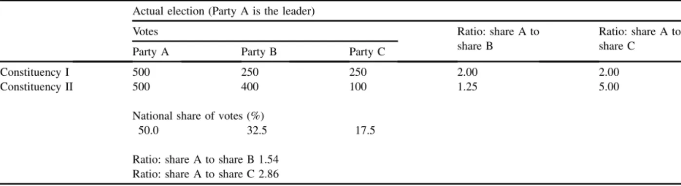
Borisyuk et al 2008 provides our interpretation of what Brookes was formulating in his bias decomposition approach (Appendix 1, pp. 4-5). In Brookes‟ original papers bias is defined as the difference between the number of seats won by the leading party – A – at

an election and the number that would be won by its main opponent – B – if B had obtained the same share of the votes. If A obtains a larger share of the seats than B

from the same share of the votes, then the positive bias favouring A is the inverse of the negative bias suffered by B.

We re-formulate the two-party Brookes‟ method in such a way that will subsequently allow extension to the three-party case. More formally, let ‘x’ be the number of seats the leading party A wins with given share, ‘k’, of the two-party vote, and ‘y’ the number of seats the second party, B, could win if it got the same share of the votes. Then, bias towards the first party is defined as the difference between the number of seats gained by this party, ‘x’, and the mean of seats gained by both parties, i.e. the mean of ‘x’ and ‘y’. Thus, for the two-party competition, bias is a function of one variable, vote share ‘k’.

Bias to party A is defined as

biasA(k) = x – MEAN(x,y) = x - (x + y)/2 = (x - y)/2 (1a)

which is simply the negative of bias towards its rival, B:

biasB(k) = y – MEAN(x,y) = y - (x + y)/2 = (y - x)/2 . (1b)

(13)

13

1. introduction of the quantitative measure of bias towards a party (difference between „x‟ and the mean of „x’ and ‘y’);

2. derivation of formulae for decomposition of bias into vote distribution effect, constituency size effect, etc.;

3. inquiry about magnitude of ‘k’that should be used if we are interested in measuring bias for a particular election; and

4. inquiry about the process whereby we might obtain the figures „x’ and ‘y’.

As part of our extension of Brookes‟ method, therefore, we explicitly address these four issues (Appendix 1; pp5-7).The first two are completely independent of any

operationalising procedure: a quantitative measure of bias that can be partitioned into separate components; and formulae for the decomposition themselves. For example, if the two main parties get equal vote shares at an election then we can calculate bias without even addressing the fourth point, the process for obtaining x and y. The reason for this is that the two parties have equal vote shares at the outset and the actual seats won can be used as ‘x’ and ‘y’. Therefore, we know that we can deal with this part of the problem (defining and decomposing bias) without discussing issues 3 and 4 above.

It is doubtful, however, that two main parties would get exactly equal vote shares at any election and the last two issues, the magnitude of „k‟ and the process for obtaining x

and y, have to be dealt with. So, we have to „construct‟ an imaginary election with

„equal conditions‟ for two parties.

Issue 3 concerns the magnitude of „k‟ that should be used when measuring bias for a

(14)

respectively if the votes actually cast were redistributed equally between them. The second, „reverse shares‟ method, on the other hand, considers what would have happened to the distribution of seats had the second-placed party (in terms of votes) obtained the vote share won by the first-placed party and the first-placed party obtained the vote of the second-placed party. In principle, it is possible to calculate bias for any

‘k’in a range between 0 and 100 (as in Johnston et al, 2002). Nevertheless, bias is usually calculated at either ‘k’=50%, i.e. equal vote shares method, or at ‘k’= actual vote share of the leading party, i.e. reverse vote shares.

Both approaches have merit. The former allows easy interpretation of bias - if two main parties get an equal share of votes but non-equal numbers of seats then the bias towards one of those parties is its „excess‟/„deficiency‟ in seats. The latter, it might be argued, retains more features from the actual electoral outcome –– size of constituencies (electoral units), turnout and minor party support variations across constituencies, as well as magnitude of national vote share, ‘k’, of the leading party. The only difference is that two main parties swap their positions – actual second party becomes new leading party with ‘k’ vote share.

The above two elements of the procedure – deriving a norm for comparison and estimating the expected number of seats for each party under certain scenarios – are clearly integral to the way in which the method is operationalised. Brookes believed that uniform swing was the simplest assumption for the first of the latter pair, but our interpretation of his original procedure is that it merely operates to construct a „norm for comparison‟, which allows us to compare data from the actual election with this

(15)

15

benchmark. It is important, therefore, that our „notionals‟ should be considered as technical steps that help in the necessary construction of the symmetrical

multidimensional distribution that retains features of the actual electoral outcome and is independent from the size of electoral area (constituency).

In the event, although this first paper re-states the Brookes method, it is a rare example of a paper being accepted for publication that fails to achieve what is sets out to do. We had decided to construct two notional elections as well as the actual election (Appendix 1 pp. 9-11) and the method appeared to work rather well for the 2005 general election which we had decided to use as the principal test of the new method. Unfortunately, when applied to earlier elections the method did not appear to work as expected! By the time this paper appeared in print we had already worked out a better procedure.

Our interpretation of Brookes‟ norm of comparison in the 2-party case is illustrated by considering the two-party percentage shares of votes cast at the 2005 British general election (i.e. [Conservative + Labour] = 100). Figure 1a shows the vote share across 627 parliamentary constituencies1 for the largest party A (Labour) and Figure 1b presents party B‟s share (Conservative). These distributions are necessarily the mirror

image of each other.2 Also indicated on both distributions is the overall vote share for each party; 52 per cent for Labour and 48 for the Conservatives.3(In both Figure 1 and Figure 2, each constituency is shown as a separate symbol.)

1_{There were 628 constituencies in Britain in 2005 but neither of the two major parties contested the}

Speaker‟s constituency.

2_{In effect the two dimensional problem can be reduced to a single dimension. Correspondingly, for the}

three-party case we can present the results in two-dimensional space.

3

These values differ from the mean values of the distribution (54% and 46% respectively) because of the unequal size of constituencies.

(16)

Figure 1.Brookes‟ two-party method: Calculation of bias.

Brookes‟ method begins by asking what would happen to the allocation of seats if instead of coming second at the actual election (AB – the parties are listed in order according to their share of the votes won, with the largest first), party B came first, receiving A‟s vote share at the actual contest. Using the principle of reverse vote shares

the method applies a uniform swing to each constituency to create a notional election result (the notional BA election) such that party B now wins 52 per cent of the two-party vote total. Following the application of uniform swing to the vote share in each of the 627 constituencies, party B‟s distribution slides to the right such that its overall

(17)

17

These three Figures 1a-c represent the conventional understanding of the Brookes‟ method. However, another interpretation is possible. Figure 1d shows the

superposition of the distribution for party A at the actual election and the distribution for party B at the notional reverse vote share election (literally, a combination of Figures 1a and 1c). This superposition is critical to our interpretation of the Brookes method because it in effect constitutes the norm for comparison and retains many important features of the actual data.

Because Brookes‟ method focuses on the two largest parties only, all constituencies lying to the right of 50 per cent are „won‟ by the respective party. Thus Figure 1a shows the number of seats won by party A at the actual election (i.e. „x‟ in previous

notation) and Figure 1c shows the number of seats („y‟) „won‟ by party B at the notional election, BA.

In Brookes‟ original formulation partisan bias towards party A is measured as the difference between the number of points to the right of 50 per cent in Figure 1a and an

average of the number of points to the right of 50 per cent in Figure 1d. It is clear from the graphs that, in effect, Brookes‟ method compares the distribution of seats at the actual AB election (Figure 1a) with the norm for comparison (Figure 1d).4

Having set out the principles underpinning Brookes‟ original formulation, we use these as the foundation for the extension to the three-party situation.

4_{For superposition AB and BA, vote shares now has zero correlation with size of constituency and has}

symmetrical shape of distribution (a norm distribution). Because of zero correlation with constituency size, the mean of the distribution equals overall vote share.

(18)

election result plus just two notional elections. The first notional election saw the actual second-placed party awarded the same vote share as the actual first-placed party (i.e. the order of the election result was changed from ABC to BAC) whereas in the second the original third-placed party was given the vote share captured by the first-placed party at the actual election (i.e. ABC was converted to CBA). The actual number of seats won was thus compared with a norm comprising the mean number of seats gained by the leading party under three scenarios – the actual election and two notional elections.

This ignored three other scenarios, and was the reason for the unresolved problems with the empirical applications. The second paper (Borisyuk et al.,2010; Appendix 2) extends the approach to incorporate the entire set of possible outcomes (i.e. including the three other potential notional elections: ACB, BCA and CAB). This extension to the three-party case does that whilst retaining many of the basic principles underpinning the Brookes‟ original formulation (Appendix 2; pp. 18-22).

Three-party vote share can be best captured by triangular graphs (for early proponents of this technique see Upton, 1976; Miller, 1977; Gudgin and Taylor, 1979; for a recent example that employs this method see Curtice and Firth, 2008). Figure 2 shows the actual 2005 election result. The point for the national three-party vote share (39, 36, 25) is represented by a cross. The area inside the triangle is divided into three, each of which shows where the respective parties won seats. Where the lines intersect at the centre of the triangle the vote share for each of the three parties is 33.3 per cent. Points

(19)

19

towards the peak of the triangle are constituencies where the largest party (in this case Labour) performed well.

Figure 2.Distribution of the three-party vote shares.

In constructing the norm for comparison for this extended procedure we have three parties, A, B and C with overall vote shares, α, β, and γ respectively,

where(α + β + γ = 100). The principle is to consider all six possible combinations assigning those three values to parties A, B and C – viz. ABC (actual election), ACB,

BAC, BCA, CAB, and CBA. This is shown on six triangular graphs (Figure 3). The first (ABC) repeats what was shown in Figure 2 while the triangle ACB below it shows the notional election where the positions of the second and third-placed parties, B and C, have been reversed but that for the first party, A, is unchanged. It is important to note that the top of each triangle always shows the largest party, the right-hand side shows the second-placed party while the third-placed party is shown on the left-hand side.

(20)

Figure 3.Distribution of the three-party vote shares: ABC (actual), ACB, BAC, BCA, CAB, and CBA (notional elections).

Figure 4 shows the superposition of these six configurations to create what will be used as the „norm of comparison‟ (Appendix 2, pp. 23-4). This procedure is a precise extension of what was done in the two-party case, where Figure 1d represented the superposition of Figures 1a and 1c. Once again, the area inside the triangle is divided into three sections The top section, for example, shows the total number of seats that

right shows seats won by whichever party came second (vote share β) while that on the left represents seats won by the third party with national vote share γ. The next stage of the process compares the actual number of seats won by each party with the expected unbiased number of seats derived from construction of the norm of comparison.

(21)

21

Figure 4.The superposition ABC + ACB + BAC + BCA + CAB + CBA. A great strength of Brookes‟ method is that it not only estimates total bias in a readily-appreciated metric but also decomposes that bias into one of four categories (Appendix 2, pp. 24-5; pp. 27-8 for the algebraic expression of these).

The first of these has been labelled differently (gerrymander, vote distribution,

efficiency) but we prefer the term „geography‟. In a „first-past-the-post‟ voting system a party performs well in the translation of votes into seats (in terms of the geography of its vote across the constituencies) by winning small and losing big; it should avoid accumulating surplus votes in constituencies it wins (i.e. those additional to the number required to win a constituency) and if it cannot win a constituency then it is best to attract as few as votes as possible there since these are literally „wasted‟(see Johnston et al., 2001).

The second component within electoral bias stems from malapportionment, i.e. differences in electorate size across constituencies (denoted by component „E‟). A party that is stronger in constituencies with relatively small electorates will tend to perform better (as shown by comparing its percentage of all votes cast and percentage

(22)

abstention („A‟) is the third component and becomes relevant when one party wins its seats where electoral turnout is low compared with its rivals whose victories are achieved in constituencies with on average higher turnouts. Finally, there is the minor party effect, component „M‟; here it is restricted to those parties outside the main three.

Brookes‟ algebra enables the contribution of each of these four components (G, E, A and M) to be calculated, in the same metric as the total bias. We derived formulae similar to Brookes‟ two-party calculations but this time for the three-party case. In the final section of the 2010 paper we examined the outcome of the 2005 general election using both the two-party Brookes method (modified to take account of third party presence) and the new three-party method (Appendix 2, p. 26).

There are a number of practical applications of this method for decomposing bias in the three-party context. One such is its application prior to and after constituency

boundary reviews (Appendix 3). Understandably, there is considerable interest in the potential political impact of boundary changes – which party(s) stands to gain and which ones might lose as electorates are equalised. However, there is a widespread misconception that boundary revisions will remove electoral bias completely and that the impact will be considerable. This depends, of course, upon the size of the

electorate bias component. In a paper published in Parliamentary Affairs we addressed this issue, maintaining that the boundary review implemented prior to the 2010 general election had largely succeeded in reducing the bias that followed from

malapportionment and that the bias which remained was a function of other

(23)

23

analysis we needed to compare the pre- and post-boundary review outcomes using the

same election. This meant first, comparing the actual election with an estimate of what the result would have been had the new boundaries been in place at the time and then, second, decomposing bias for each of those elections (Appendix 3, pp. 44-8).

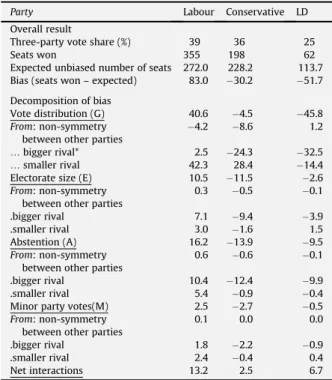
A further application of the new three-party bias method came with a recent paper published in 2012 that reviewed UK general elections since 1983 (Appendix 4). Although these elections had been examined before this was an opportunity to examine what the new method would reveal in terms of the trend in the composition and

contribution of bias – was geography becoming more important and if so, for which party? Table 2 in that paper (Appendix 4, p.58) describes the evidence.

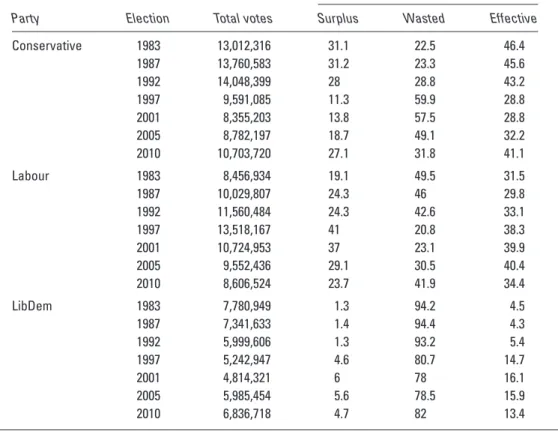
Although it is standard practice when considering the geography or vote distribution bias component to identify surplus and wasted votes separately, in this paper we began to advocateinstead a catch-all concept of „ineffective votes‟ since this may provide greater insight into how that bias develops in practice (Appendix 4, pp. 60-2). Another important contribution set out in this paper is a series of graphs that seek to highlight the occasions when votes are/are not converted into seats. Although not shown here in colour (the published version does use colour) there are clear advantages in aiding understanding using this type of visualisation (Appendix 4, pp. 64-6). A much more detailed example of our approach to data visualisation can be found in a paper that decomposes bias for the 2010 general election (Thrasher et al. 2010).

There is no disputing the fact that electoral bias is of considerable interest in the UK political context. There is also no disputing that few people appreciate the complexity

(24)

party case this research has tried to explain what electoral bias is (especially in the sense that it is not equivalent to disproportionality) and those separate and sometimes conjoined elements that comprise it. The intended audience is broader than the

academic community of electoral geographers and political scientists because it matters that a wider public understand the reasons that lie behind situations when there is an asymmetry in the electoral battleground where one party requires only a narrow lead over its rivals to win an overall majority whereas another party needs a much larger lead.

It has been particularly important to demonstrate that the impact of boundary changes in removing bias is directly linked to the extent of bias contributed by unequal

electorates; the criticism levelled towards the independent boundary commissions has often been unjustified. Given the radical nature of proposed boundary changes to be implemented prior to the 2015 general election it is likely that interest in electoral bias among both academics and the wider public will continue.

2. Patterns of voting and party competition in London Assembly Elections

Occasionally, opportunities for interesting and novel research arise when particularly good data become available. One example of this relates to the elections for the

Greater London Authority (GLA) which used electronic counting methods to determine the winner of its mayoral and assembly contests. London Elects, the body responsible for conducting these elections, released the 2004 data in machine-readable format using

(25)

25

London borough wards as the lowest level of aggregation. Rallings and Thrasher were working with Henk van der Kolk, principally looking at the supplementary vote system used for electing the mayor but when the 2004 data were published this opened up new research possibilities.

One of the principal weaknesses of UK election surveys, such as the British Election Study, is that the number of voters that support the smaller parties is often too small to obtain a sufficiently large number of responses. A major weakness of aggregate data analysis is that such parties also do not necessarily contest many seats, particularly in local elections where the number of vacancies is very large. This obstacle disappears when small parties are required to select a relatively small number of candidates but when many electors are eligible to vote for them. This circumstance arose in the case of London when small parties could provide lists for both the Assembly and European elections and when the data became available at the ward level.

The 2004 London elections coincided with elections for the European Parliament which meant Londoners could vote five times (two votes for London mayor, London

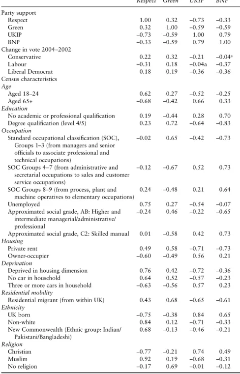
constituency vote, London-wide list vote and the European vote). Since 1999 the UK has used regionally-based electoral districts for European elections but uniquely these voting figures became available at much smaller levels of aggregation than normal. Before we could undertake any analysis, however, it would be necessary to construct a usable data set (Appendix 5, pp.82-4). As well as using the ward-level voting data we added some demographic characteristics and also local voting figures. A combination of statistical procedures (Appendix 5, pp.86-92) began to build the case that there were patterns in support cast for the different minor parties (Respect, Green, UKIP and BNP)

(26)

highlighting where those differences were. Accordingly, I used GIS to construct ward maps of the London European vote which did succeed in revealing how the votes were spatially clustered across London (Appendix 5, pp.94-6). Mapping permitted us to see clear spatial patterns in voter support for the Greens, Respect, UKIP and the BNP respectively.

When the 2008 results also became available we decided that we could test the proposition that small parties can benefit from opportunities provided by the parallel implementation of separate voting systems. In London elections to the 32 London boroughs are conducted by simple plurality, making it difficult for small parties to find candidates and difficult to attract votes. By contrast very few candidates are required to contest the London-wide list seats. Given that the 2004 data were available at the ward level would a party like the Greens, for example, note those areas where there was support and then use that information to establish target wards in time for the following local elections.

Compiling the data set meant merging separate files for 624 wards containing London borough election results for 2002, 2006 and 2010 and the London Assembly voting figures for 2004 and 2008 (Appendix 6, pp. 110-3). Multiple binary logistic regression was used with the first set of data 2002 - 2004 – 2006 to build a model while the second cycle, 2006 – 2008 – 2010 could be used for out of sample testing (Appendix 6, pp. 107-10). Once again, we used GIS to map Green support across London (Appendix 6, pp. 113-5). The analysis concluded that it did not appear that the Greens did make use

(27)

27

of the potentially valuable data provided by the London list-vote data when identifying areas where local election candidates could stand and perhaps attract voter support.

3. Electoral forecasting

An important strand of the activity undertaken by the Elections Centre surrounds the topic of election forecasting. Rallings and Thrasher chose to take an entirely different route to most other election forecasters, preferring to use local election data to generate forecasts, first for the purposes of making predictions about local elections (Rallings and Thrasher 1996) and later to extend the method to general election forecasting (Rallings and Thrasher 1999). After joining the Centre I worked on a method based on Neural Networks (Borisyuk 2005) and although this had some success and recognition we have returned to the aggregate local electoral data for generating national forecasts.

Using local council by-election data to generate these forecasts provides an alternative source to national polling data but presents real challenges. Over recent years we have addressed the problems associated with varying patterns of party competition

(Appendix 7, pp. 122-5) and it is fair to say that for us this continues to be a „work in progress‟. Recent modelling has also incorporated opinion poll data, largely as a benchmark for comparison and for this purpose I developed a method of weighting data to take account of the different polling companies undertaking surveys with different frequencies (Appendix 7, pp.126-7). The model developed for the 2010 UK general election produced a GB national vote share forecast of Conservative 36% (actual 37%), Labour 28% (30%) and Liberal Democrats 28% (24%). The seat forecast was

(28)

At least we correctly forecast the hung parliament!

Following the lessons of 2010 we have begun to explore the possibilities of generating forecasts that take account of the impact of different configurations of party

competition, i.e. Con versus Lab; Con versus LD etc. We may also return to the Neural Networks approach (Borisyuk et al 2005) or use another method entirely.

4. Space, Place and Ballots

This section has a rather catch-all description but the category reflects one of the great strengths that the Elections Centre brings to the study of voting behaviour in the UK. Over a period of more than 25 years the Centre has developed probably the world‟s most extensive collection of aggregate local election data. Extracting data sets from this complex database requires considerable skill and patience but the rewards are that we can address important issues, ranging from the under-representation of women (Appendix 8), voter turnout (Appendix 9), and the effect of voting procedures on voter behaviour (Appendices 10 & 11).

When we examined the presence and performance of women candidates in local

government there were a number of data issues to resolve (origin time given differences in local government reorganisation, structural reforms in local government, complex electoral cycles etc. - Appendix 8, p. 136). The analysis first considers women candidates (Appendix 8, pp. 137-41) and addresses the „contagion‟ question – do

(29)

29

parties select women candidates when rival parties do so and the balanced ballot – when parties can select candidates in multimember wards do they strive for some level of gender balance. The second part of the paper tracks the pace of change in women‟s election before examining the relative performance of men and women candidates within party slates (Appendix 8, pp. 141-3). It appears that voters do not discriminate either for or against women. In the final section we addressed questions about tenure – are women councillors more likely to retire from office than are men and when male incumbents retire do local parties select women to replace them? The general

conclusions derived from this analysis are that women are not discriminated against by voters and probably not by party selection processes leaving the most likely

explanation of women‟s recruitment to be resource-based.

Exploring the relationship between voter turnout and geography has led to a valuable collaboration between the Elections Centre and Scott Orford of Cardiff University (Orford et al 2008, 2009, 2011). In low information elections we expect that voters take more account of the associated costs of voting than they might do when

participating at a general election. The challenge lay in organising data that would permit the test of that hypothesis. A handful of local authority election officers retain detailed records of voter turnout for each polling station. One such was the London borough of Brent. We obtained these data for a twenty year period. Over this period voters had (or had not) participated in borough council, European parliament and general elections. Orford created maps of the polling station areas and we used different measures of distance (Euclidean, topography etc.) and population density in order to estimate average distances to polling station for in-person voters (Appendix 9, pp. 160-4).We finally decided to use multi-level modelling (voters are based at polling

(30)

turnout for the three types of election. The analysis shows the effect on turnout at the aggregate level of such factors as deprivation and age while noting that European election turnout is most affected by network distance and local election turnout relates to ward marginality (Appendix 9, pp. 166-72).

In recent years I have also been analysing individual-level data compiled from the annual surveys of local election candidates undertaken since 2006. This research has led to reports (Rallings et al 2007; 2009; 2010) and articles in peer-reviewed journals (Rallings et al 2010; Thrasher 2012 forthcoming) with the academic output likely to increase as the annual data are pooled and examined in more detail. Much of this research is policy-oriented addressing issues of contemporary importance (for example, the under-representation of women, younger people and minority ethnic populations).

It is a feature of the research process that one line of inquiry often leads to another. This is the case for two related papers that examine a common phenomenon in local elections where voters are invited to fill multiple rather than a single seat. The first paper (Appendix 10) demonstrated that between 7-15% of total potential votes in English council elections using a block vote system remain unused; some voters with three votes, for example, would opt to use only one of them. Was this because highly partisan voters would refrain from using votes when their chosen party failed to field a full set of candidates? If not, what clues might be found from the election data that might indicate some of the causes of unused votes. Invariably, before addressing the question there were data issues to be resolved (Appendix 10, pp. 180-1).

(31)

31

We were able to demonstrate that the structure of party competition does not wholly explain the absolute level of unused votes (Appendix 10, pp. 181-3). Another line of inquiry was then pursued. Was there possible evidence that some voters might not understand how the voting system worked and might imagine that they had only a single vote to cast? Indeed, there was a strong alphabetic advantage for candidates placed near the top of each ballot paper (Appendix 10, pp. 184-6) that was only partly mitigated by incumbency factors. An ordinal logistic model (Appendix 10, pp. 188-92) provides strong evidence for an alphabetic bias. In the final part of the paper (pp. 193-5) we construct a regression model using the percentage of unused votes as the

dependent variable and predictor variables that take account of the ward context (party competition and demographic characteristics). Decisions by local parties not to field a full slate of candidates has a large impact on the proportion of unused votes but there was also no disputing the evidence that support for candidates was affected by their order on the ballot.

Appendix 11 builds directly on the conclusions reached in this earlier paper and tests the extent of alphabetic bias in local council elections over a forty-year period. The data incorporated the names of 657,704 candidates that stood in 164,333 separate ward elections. The analysis provides stronger evidence than before about the extent of alphabetic bias, the relationship with the size of the block vote (bias increases as district magnitude rises) and the number of candidates standing (Appendix 11, pp. 207-13. The logical consequence of this, of course, is that candidates placed near the top of the ballot have a better prospect of gathering votes than do lower-placed candidates and therefore have a better chance of being elected. We tested this using Richard Webber‟s name origins software which reports the distribution of surnames currently within the UK (Appendix 11, pp. 216-7). We found that compared with the general population

(32)

deciles. To remove this bias we recommend the practice used elsewhere of ballot order randomisation for UK elections.

5. Candidate recruitment

Although most of my work has been undertaken while using aggregate data there are some recent exceptions. In 2006, Mary Shears of the Elections Centre introduced a national survey of local election candidates. The survey has been conducted annually since then with candidates selected randomly from nomination lists and invited to participate. About one thousand responses are collected each year and I have pooled these data noting where the same or similar questions have been asked. I have also combined the individual-level data with ward and authority-level measures and weighting data to correct for response bias (see Appendix 13 for a more detailed description of this procedure).

Two recent publications are included here (Appendices 12 & 13) that reflects the kind of research that is being undertaken with these data. I noted earlier (Appendix 8) that the aggregate data analysis of women‟s under-representation in local government could only advance our knowledge to a certain extent. Appendix 12 aims to take the analysis a step further by, inter alia, discovering from women candidates some of the processes that brought them to stand, the support they received from others and whether their experiences were different to those of men. It appears that women are less likely than men to take the decision to stand; they are more likely to be asked to stand. By contrast,

(33)

33

the relatively small group of non-white candidates and those aged below 45 years that stand are more likely to make their own decision (Appendix 12, pp. 231-3). As far as the candidates are concerned the problems of under-recruitment lie mainly with supply-side issues coupled with a feeling that local parties might be doing more to select members of these under-represented groups.

For the paper examining ethnic candidates in local elections (Appendix 13) we again collaborated with Richard Webber, using his OriginInfo software to identify candidate ethnicity. This was partly to test his software reliability and partly to consider the nature and extent of sample/response bias for the Local Candidate surveys. The first part of the paper, therefore, (Appendix 13, pp. 247-8) uses the software to classify the ethnic origins of all candidates standing for election. Next, we compare the list selected to be invited to complete a questionnaire with all candidates in order to measure any sample bias. Because we use random sampling we were reasonably confident that such bias would be avoided and we were correct in this interpretation. The next procedure was to test for response bias by comparing the list of candidates that did or did not respond. This provided evidence of response bias with a lower response rate from Black, Asian and other minority ethnic candidates. The subsequent analysis was able to correct for this bias.

BME candidates are more likely to be younger and better educated but fewer women are recruited from among this group. Such candidates are electorally inexperienced, have stronger ties with community related organisations and are more likely to make their own decision to stand for election rather than being approached by a fellow party member. Community ties are also evident when respondents are asked about their

(34)

experiencing positive support from this quarter (Appendix 13, pp. 256-7).

General Discussion

These research papers seek to expand our understanding about voters and parties in Britain. Generally speaking, the research has relied upon aggregate data (especially local and parliamentary election data) but in recent years I have been working extensively with survey-level data also. These different types of data present rather separate challenges. One continuing task with the aggregate data is to check for errors and inconsistencies and, where possible, to amend the original records. When the number of candidates and elections numbers in the many thousands as happens with the local elections this can be a daunting task, particularly when the contests occurred decades ago. One major task has been the treatment of missing data. For example, one important piece of information that local authorities often failed to record was the number of ballot paper issued for elections to multimember wards. This was handled by an algorithm that took account of various patterns of party competition. A similar approach was used for the electoral forecasting model when local parties began to withdraw candidates from these contests (see Appendix 7) and in weighting opinion poll data when the frequency of polls began to vary widely.

The survey data present different kinds of problems as anyone who has worked with these types of data can attest. In one sense, however, our recent work has transformed this „necessary chore‟ into a research programme in its own right. Recent papers that

(35)

35

have used the annual candidates‟ survey have described the methodological innovations that we have developed to measure any sampling bias and, more importantly perhaps, the nature and extent of response bias. These papers have also united the aggregate and individual-level data analysis because we are extending our application of name

recognition software from the survey to the aggregate data in order to explore the relationship between candidate ethnicity and patterns of vote distributions.

Facing and solving challenges in the research process often leads to methodological innovations that were not planned but instead evolved. The papers included in the first section on electoral bias, for example, provide a useful description of this process. It began with an initial discussion about the limitations of the Brookes method for three party competition in Britain and the need to search for a more effective approach to decomposing bias. One of the papers included here is rare amongst academic publications – a description of a research process that ultimately failed. But the failure led us to reassess our original thinking and then to develop a successful methodology. In turn, that methodology was then applied and has hopefully expanded our

understanding of the operation of the different bias components at UK general elections from 1983 onwards.

At other times research in one area has stimulated research that takes another direction. This can be illustrated by showing how the study of unused votes led us eventually into the field of candidate ethnicity. When the research was originally envisaged the central problem lay in identifying the scale of unused votes in British local elections – how many people when given more than a single vote were making full use of those votes. It was only after considering this that our focus turned to the examination of patterns in

(36)

rewarding candidates placed at or near the top of ballot papers organised in order of candidate surnames that attracted the attention of Richard Webber. His own interest lay in the ethnic origins of surnames rather than their positioning in both the alphabet and specifically on ballot papers. The paper included here as Appendix 11 is the first in what promises to be a rewarding research collaboration. We are already working on a paper that after using the name recognition software to classify candidates as British white/other white/non white then considers the relationship between candidates‟ ethnic origins and vote change (in the case of single member wards) or finishing party

position order (in the case of multi-member wards). Ultimately, for the UK context, we hope to be able to answer the question – does a candidate‟s name on the ballot affect the distribution of votes and what is the direction, strength and impact of that

relationship?

Further collaboration with Scott Orford and the geography of voting is also being undertaken. This research is another demonstration of how we are merging aggregate and individual-level data and applying multi-level methods. The focus of this research will be on local election candidate recruitment and the relationships between a

candidate‟s residence and the location of the ward that is being contested. We know from the candidates‟ surveys that just under half of all candidates (the figure is lower for councillors) live outside the ward that they contest. We also know that around one in four are „paper‟ candidates, agreeing to stand on condition that there is no prospect of winning. What we do not know, as yet, is in the cases where residence lies outside ward boundaries whether the two areas are close to one another or not and how that geography varies across the country. Is it the case that parties try, where possible to

(37)

37

select candidates that if not a ward resident are at least living close by, or are (some) parties mainly concerned with finding names to include on the ballot paper?

Finally, it is worth noting the extent to which this research impacts or seeks to impact upon the real world of politics and policy making. It is understandable that during UK general elections that people become interested in explanations that account for

asymmetries in vote/seat distributions. The value of extending the Brookes‟ method is that we can show how far one party‟s advantage is a function of say, unequal

electorates, and how other factors contribute also to that bias. Much of our work addresses practical issues. If ordering ballot papers according to candidate surname affects the distribution of votes should be rotate those names randomly as happens in other countries? Given that women and minority ethnic candidates are

under-represented in local elections is the best approach for remedying that situation to address supply or demand issues? If the location of polling stations directly affects the proportion of voters that participate in certain kinds of low salience elections and expanding the pool of postal voters is not a positive option then how can we optimise those locations to improve turnout? Political science does not have to be relevant to be important but when it can address such questions empirically then it should.

(38)

References

Katz, R. (1997) Democracy and Elections. New York: Oxford University Press. Monroe, B. L. (1994) Disproportionality and Malapportionment - Measuring Electoral

Inequity. .Electoral Studies 13 (2): 132-149.

Orford, S., C. Rallings, M. Thrasher & G. Borisyuk (2008) Investigating differences in electoral turnout: the influence of ward-level context on participation in local and parliamentary elections in Britain. Environment and Planning A, 40 (5): 1250-1268.

Orford, S., C. Rallings, M. Thrasher, & G. Borisyuk (2011) Changes in the probability of voter turnout when resiting polling stations: a case study in Brent, UK.

Environment and Planning C: Government and Policy 29 (1): 149-169. Rallings, C., and M. Thrasher (2011) Election 2010: The Official Results. London:

Biteback Publishing.

Rallings, C., M. Thrasher, & G. Borisyuk (2010) Much ado about not very much: The electoral consequences of postal voting at the 2005 British general election.

British Journal of Politics and International Relations 12 (2): 223-238.

Rallings, C., M. Thrasher, G. Borisyuk, & M. Shears (2007) The 2007 Survey of Local Election Candidates. London: Improvement and Development Agency.

Rallings, C., M. Thrasher, G. Borisyuk, & M. Shears (2009) The 2009 Survey of Local Election Candidates. London: Improvement and Development Agency.

Rallings, C., M. Thrasher, G. Borisyuk, & M. Shears (2010) The 2010 Survey of Local Election Candidates. London: Improvement & Development Agency.

(39)

39

(40)

(41)

A 1

Appendix 1

Measuring bias: Moving from two-party to three-party elections

Borisyuk, G., R. Johnston, M. Thrasher, & C. Rallings (2008) Measuring bias: Moving from two-party to three-party elections. Electoral Studies, 27 (2), 245-256. 55% of the work for the paper was undertaken by Galina Borisyuk

A copyright permission request to include this paper in the submission was made to and granted by the publisher Elsevier.

(42)

(43)

Measuring bias: Moving from two-party to three-party elections

Galina Borisyuka,, Ron Johnstonb, Michael Thrashera, Colin Rallingsa

a

LGC Elections Centre, University of Plymouth, Drake Circus, Plymouth PL4 8AA, UK b

Department of Geographical Sciences, University of Bristol, Bristol, UK Received 4 April 2007; revised 9 November 2007; accepted 10 November 2007

Abstract

One method for assessing the extent of electoral bias is that first developed by Brookes. This method decomposes bias into dif-ferent elements, including efficiency of vote distribution as well as effects separately produced by electorate size and turnout. Brookes’ method is used to measure electoral bias largely in two-party systems but the rise of third parties, particularly in recent UK elections, has prompted the search for a reliable alternative. This paper reports upon findings from an on-going research pro-gramme. The nature and theoretical underpinnings of different procedures that might be used for decomposing bias in the three-party case are outlined. Two main procedures are constructed and then tested against the results from actual elections. The evidence shows that these procedures produce similar findings in respect of the 2005 general election but differences emerge when earlier elections are considered. Research continues to assess whether these differences follow from the nature of party competition at each election or the particular procedure employed.

Keywords:Electoral bias; Electoral geography; Third parties

1. Introduction

A well-known feature of simple plurality electoral systems is that, irrespective of any explicit political involvement in drawing district boundaries (the malap-portionment and gerrymandering strategies char-acteristic of much redistricting in the United States), legislative contest outcomes are almost invariably

disproportionaldmore so than with many other types

of electoral system. Such disproportionality usually

favours the largest of the two main parties whichdas

identified from Duverger’s classic work (Duverger,

1954) onwardsdtend to dominate such systems.

What is not as well attested is whether that dispropor-tionality is unbiased by not treating these two largest parties differentially. A system that gives the largest party a ‘winner’s bonus’, with, say, a ten percentage points greater share of the seats than of the votes, is

disproportional. However, if main partyAobtains that

bonus but main party B, with the same vote share,

gets a bonus of only five points, then the system is

not only disproportional but also biased towards A.

Such a winner’s bonus is sometimes termed

exaggera-tion (Johnston et al., 2002) or responsiveness (King,

1990), or majoritarian bias (as inCalvo and Micozzi,

2005), and it differs from ‘electoral bias’ (Johnston

_{Corresponding author. Tel.:} _þ_{44 (0)1752 232619; fax:} _þ₄₄ (0)1752 232785.

E-mail addresses:[email protected](G. Borisyuk),

[email protected] (R. Johnston), mthrasher@plymouth. ac.uk(M. Thrasher),[email protected](C. Rallings). 0261-3794/$ - see front matterÓ2007 Elsevier Ltd. All rights reserved. doi:10.1016/j.electstud.2007.11.011

Available online at www.sciencedirect.com

Electoral Studies 27 (2008) 245e256

www.elsevier.com/locate/electstud

(44)

et al., 2001) or ‘partisan bias’ (Grofman and King,

2007) which refers to an asymmetry in the way party

vote share is translated into seats (the same share of the votes cast can result in substantially different shares of the seats). We will consider electoral bias only and refer to it as simply bias.

An unbiased system, according toGrofman and King

(2007), is characterised by what they termpartisan sym-metry(see alsoKing et al., 2005), a requirement that

‘. the electoral system treat similarly-situated

parties equally, so that each receives the same frac-tion of legislative seats for a particular vote percent-age as the other party would have received if it had the same percentage’.

Grofman and King (2007, p. 6)claim that this defini-tion of partisan symmetry has been virtually the consen-sus position of social scientists as a means of assessing the partisan fairness of a districting scheme. Measuring it has been a cause of considerable experimentation and

debate, however: asKing et al. (2005, p. 9)note:

‘A consensus exists about using the symmetry stan-dard to evaluate partisan bias in electoral systems. But such a consensus does not answer the subsidiary question: how to measure symmetry itself in order to determine whether partisan bias exists’.

(Hence the experimentationdas in King, 1990;

Gelman and King, 1994; Grofman et al., 1997; Gelman et al., 2004dsome of which has sought only to identify the extent of bias, without also decomposing it to

un-cover its sources.1)

One procedure used to measure that bias was

devel-oped in New Zealand by RalphBrookes (1953, 1959,

1960), which has the major benefits of using a readily-appreciated metric and being decomposable into the various bias sources that he identified (variations in con-stituency size, abstention rates, voting for third parties,

and the distributions of party support).2It has been widely

applied to the analysis of British election results in the last

two decades (e.g. Johnston et al., 2001, 2002, 2006).3

Brookes’ method was ideally suited to the analysis of

a system where two parties predominateddas was the

case in New Zealand until the 1990s: it assumes that

other parties gain a proportion of votes cast thatcannot

be translated into seats. Its application to British elec-tions since 1974 is thus constrained by the growth of ‘third party’ votes in England and ‘fourth party’ votes in Scotland and Wales that were subsequently translated into seats. Although a third party victory component

was added later by Mortimore (1992): (see Johnston

et al., 1999) to get a more realistic appreciation of the extent, direction and sources of any observed bias, nev-ertheless the method essentially remains focused on the

two-party situation. Brookes’ methoddalong with most

others seeking both to identify and decompose the level

of biasdtreats third parties as, in effect, the source of

relatively small amounts of ‘noise’ in a predominantly two-party system. Our goal here is to undertake a further modification of the method of decomposing bias that will make it better suited to the realities of three-party competition, where each of the parties is competing with the other two (perhaps in different places) for sub-stantial numbers of votes and all three are potential seat-winners. This paper represents the initial stages in this process.

2. Reformulating Brookes’ measure

In this paper, we re-formulate the two-party Brookes’ method in such a way that will subsequently allow extension to the three-party case. More formally,

letxbe the number of seats the leading party wins with

given share,k, of the two-party vote, andythe number

of seats the second party could win if it got the same share of the votes. Then, bias towards the first party is defined as the difference between the number of seats

gained by this party, x, and the mean of seats gained

by both parties, i.e. the mean of xandy. Thus, for the

two-party competition, bias is a function of one

vari-able, vote sharek.

Bias to party A is defined as

biasAðkÞ ¼xMEANðx;yÞ ¼x ðxþyÞ=2

¼ ðxyÞ=2 ð1aÞ

which is simply the negative of bias towards its rival, B:

biasBðkÞ ¼yMEANðx;yÞ ¼y ðxþyÞ=2

¼ ðyxÞ=2: ð1bÞ

Although Brookes’ method of measuring bias is often considered as based on electoral outcomes of uniform

1 _{Grofman and King (2007, p. 32)}_{do claim, however, that ‘The} de-gree of deviation from symmetry of treatment is known aspartisan bias, and is easily quantified, and made specific as to direction’.

2

An alternative approach, developed almost contemporaneously with Brookes’, identifying the same basic bias components, isSoper and Rydon (1958), who developed early ideas ofBrookes (1953).

3

The only other attempts to measure and account for bias in the UK have been those byCurtice (2001)(see alsoCurtice and Steed, 1986), which although it identified the various sources of bias did not quantify their relative importance in terms of seats, and Blau’s important critique of Brookes’ approach (Blau, 2001) and his sugges-tion to use an ‘integrated method’ (Blau, 2001, 2004).