Portelli, K. and Anagnostopoulos, C. (2017) Leveraging Edge Computing through
Collaborative Machine Learning. In: 2017 5th International Conference on Future
Internet of Things and Cloud Workshops (FiCloudW), Prague, Czech Republic, 21-23
Aug 2017, pp. 164-169. ISBN 9781538632819.
There may be differences between this version and the published version. You are
advised to consult the publisher’s version if you wish to cite from it.
http://eprints.gla.ac.uk/142024/
Deposited on: 6 June 2017
Enlighten – Research publications by members of the University of Glasgow
http://eprints.gla.ac.uk
Leveraging Edge Computing
through Collaborative Machine Learning
Kurt Portelli
School of Computing Science University of Glasgow, G12 8QQ UK
Christos Anagnostopoulos School of Computing Science University of Glasgow, G12 8QQ UK [email protected]
Abstract—The Internet of Things (IoT) offers the ability to analyze and predict our surroundings through sensor networks at the network edge. To facilitate this predictive functionality, Edge Computing (EC) applications are developed by considering: power consumption, network lifetime and quality of context inference. Humongous contextual data from sensors provide data scientists better knowledge extraction, albeit coming at the expense of holistic data transfer that threatens the network feasibility and lifetime. To cope with this, collaborative machine learning is applied to EC devices to (i) extract the statistical relationships and (ii) construct regression (predictive) models to maximize communication efficiency. In this paper, we propose a learning methodology that improves the prediction accuracy by quantizing the input space and leveraging the local knowledge of the EC devices.
Keywords-edge analytics; predictive intelligence; edge com-puting; collaborative machine learning;
I. INTRODUCTION
An IoT environment comprises billions of interconnected sensing and computing devices, things, which sense and share contextual information, hereinafter referred to as con-text. Contexts are also capable of performing localized analytics like linear regression, outliers detection, and clas-sification. Things include anything ranging from smart-phones, military sensors [1], to Radio Frequency Identifi-cation (RFID) tags found in everyday products. As more contextual data are made available, opportunities arise for analytics and statistical learning applications that extract context information and reason about it. The smart grid has been recognized as an important form of IoT since it allows a two-way contextual information flow which produces new perspectives in energy management[2]. Furthermore, there is an interest for the visualization of a tactical battlefield that can only be achieved through contextual data collected from sensor networks. Making all this context interpretable and useful is challenging as it needs to be sensed, collected, inferred, transferred, and stored [3].
To extract and infer contextual information from the IoT network edge, contextual data is read from sensor & actuators nodes, which measure the temporal-spatial field of a specific area. Contextual (scalar) parameters can be e.g., humidity, temperature, wind speed. This context is then
relayed to a sink node, hereinafter referred to as sink (back-end-system) for further processing and inference [4]. The back-end-system has access to more computational power compared to sensing nodes. In a traditional system, all these sensors generate massive amounts of context and, periodically, transmit it to the sink. In turn, sink restructures the data more effectively to transmit them to another system further up the hierarchy or locally stores them for further processing and/or analytics tasks, e.g., regression analysis. However, in this scenario, the IoT network transfer drains power and, as the network scales, this effect is emphasized even more. This motivated us to depart from the traditional system and to propose an approach forpushing intelligence it terms of machine and statistical learning [5] to theedge of the network and close to the source of the contextual information as possible in a collaborative manner. L.Bottou et al. [5] state that large-scale incremental machine learning attempts to outrun the exponential evolution of computing power. This paper shows that in the case of edge-centric col-laborative machine learning, incremental (on-line) learning algorithms on the network edge are capable of processing large amounts of contextual data with comparatively less computing power and less network overhead when compared to the traditional sensor-back-end systems approach. A. Related Work & Contributions
The baseline approach for regression analytics tasks (like prediction and classification) on the cloud is to periodically transfer all the raw data from each sensing device of the edge. The back-end-system located on the cloud has no power consumption limitations and has access to more computing resources when compared to the sensors, thus, performing advanced analytics once the data is collected. As previous studies have outlined [6],[7], [8] this approach is very straightforward to implement but has gross disadvan-tages, such as high energy consumption and high network bandwidth due to the streaming of raw data over the edge network. To tackle these disadvantages, we refer to EC [9], which pushes the computation away from the cloud to the edges of the network. Our approach is to adopt this methodology by placing the computational logic inside the
sensors (in-network intelligence) away from the back-end-system. F. Bonomi et.al [10] describe EC as a large number of nodes geographically distributed supporting real-time in-teractions, wireless access, and heterogeneity. Furthermore, on-line regression analytics are the essential component for EC due to the requirement of context awareness in IoT environments. M. Rabinovich and Z.Xiao [11] describe an application content delivery network based on EC. They produce a middleware platform for providing scalable access to Web applications. Currently, EC is being promoted as a strategy to achieve highly available and scalable Web services. [12] Our intention is to extend the functionality of EC and enable contextual regression analytics tasks in-network accessible from the back-end-system while, at the same time, maximizing network efficiency and quality of analytics.
Contributions: In this work, we propose a novel
col-laborative machine learning model at the IoT network edge that achieves both: (i) highly accurate prediction results over regression analytics tasks and (ii) scalability of the IoT edge network. Using incremental machine learning on the network edge, our methodologyexploits the relationship of the con-text collected to extract knowledge and predict new concon-text. Instead of transmitting raw contextual data in the network, weonlytransmit the inferred knowledge, i.e., the minimum sufficient statistics, which encapsulates and approximates the underlying data at the edge. [Desideratum 1:] Our rationale is based on the idea that each computing and sensing device, independently trains an on-line, local, linear regression model, which is then transferred to the back-end-system. This ensures network efficiency by avoiding transmitting the data; only meta-data corresponding to model parameters. The system then has access to all the received local models and, when queried for certain prediction / analytics queries, it has to intelligently select which model(s) to engage. [Desideratum 2:] We acknowledge that the received regression models from all the edge nodes might not be equally accurate amongst all the input space during the analytics tasks. Hence, we further adopt adaptive vector quantization to intelligently determine and aggregate the best regression models for each subset of the input space. We provide a comprehensive performance and comparative assessment to showcase the applicability of our model in terms of prediction accuracy and quality of regression results in the IoT network edge.
II. RATIONALE& PROBLEMDEFINITION
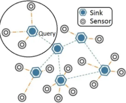
We consider an EC/IoT environment with a set of sensors (edge nodes) and sinks with paths leading from the sensors to the sinks. Sensors are only connected with one sink with the aim of the network being to transfer captured context to the back-end-system, which is the entry point to a cloud system. Let us focus on one instance of the whole network
Figure 1. EC/IoT environment with a network of computing/sensing nodes (sensors) and sinks supporting regression analytics tasks.
as shown with the black circle in Figure 1; although our concepts are extended to the entire network.
Each sensor Si gathers data contextual about the space
around it. Each contextual datum at time t consists of the multivariate vector x ∈ Rd, which is referred to as
input and scalar y ∈ R, which is referred to as output. Vectorxand scalary can represent any data sensed by the sensor, e.g., temperature, humidity, acidity, luminosity, CO2
concentration, where we seek to learn the local regression functionfi : x→y at nodeSi. The pair(x, y)comprises
the context at sensorSiat timet. Each sensorSicaptures a
stream of pieces of context{(x`, y`)}∞`=1. One of the main
challenges is the collection of context from the sensors [3]. Both vectorxandy are part of the contextual information sensed from Si at time instance t, such that sensor Si
models the relationship betweenx and y by observing the data in real-time and extracting the local regression function
fi(x) =y.
Multivariate stochastic gradient descent [5] is a model used to incrementally learn the fi from multiple pieces of
context on each sensorSi. Assuming that there exists a linear
relationship, this linear model allows us to predict y based on the inputx. The hypothesishθ(x)of thed-dimensional
linear model is defined in (1). The θi = [θ1, . . . , θd]>
represents the weights of the local linear regression function, i.e., determine the mapping between each xi and y. As
sensor Si captures context the weights are updated in an
on-line fashion as explained in [5].
hθ(x) =θ0+
d
X
k=1
θkxk (1)
Challenge 1: Sinks store context pairs of each of their
connected devices and allow access through querying. The baseline solution is to transfer all the data pairs(x, y)from the sensors to the sink and then learn one global linear regression modelat the sink. We argue that this is inefficient as all the context pairs must be transmitted over the network.
Problem 1: Given a set of sensors at the network edge,
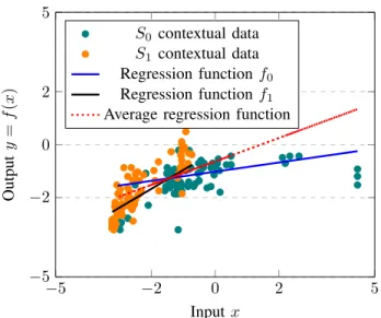
−5 −2 0 2 5 −5 −2 0 2 5 Inputx Output y = f ( x ) S0 contextual data S1 contextual data Regression functionf0 Regression functionf1
Average regression function
Figure 2. Linear regression example with two local regression functions f0andf1from sensors’S0andS1contextual data, respectively, and global
regression function at the sink/back-end-system.
functions fi for each sensor Si and efficiently update the
back-end-system without transferring contextual data in the network.
Challenge 2: Now, the purpose of regression analytics
tasks in EC is to query a system and then provide us (e.g., analysts, data scientists) with predictions. The regression analytics query we are dealing with is of the formq= (x)
and we expect prediction output yˆ as a result [6]. In the ideal scenario, the back-end-system knows which sensorSi
to use for the prediction of y, so it can directly apply the corresponding functionfi given a queryq(x). However, in
real-life applications this is not possible, thus, the average prediction is used, i.e.,q(x) = ˆy=n1Pn
i=1fi(x). Consider
the raw contextual data of two sensors in Figure 2, where we can observe the local linear regression functions of both sensorsf0 andf1, and the average regression line f1+2f2. It
is obvious that the average line is heavily biased by sensor
S0, thus, certain ranges ofxmapped by sensorS1’s function
are not supported. We argue that the average is not ideal in most scenarios and instead should adopt a methodology to optimally choose the models that obtain the minimum error. The back-end-system has access to all the contexts of the connected sensors. For each query q(x), a simple solution is to predict the result using the average from all local functions, but as above-mentioned from our example, not all local regression models have been trained on the same subset of the input space x. This raises the challenge on whether for each queryq(x)there exists anoptimal subsetF
of these regression models, which is more accurate than the average of all models in terms of prediction error. Departing from Problem 1, in which we have efficiently learned the local regression models fi, we have to cope with finding
this optimal subset of models in light of minimizing the prediction error on the sink node.
Problem 2: Given a set of trained and up-to-date local regression functions fi at the sink, find a methodology
to select a subset F of those functions to minimize the prediction error w.r.t. the average regression model.
III. EDGE-CENTRICLEARNING
Resources in a sensor are reserved for communication, processing and data sensing. It has already been established that data transmission consumes much more energy when compared to the processing and data sensing tasks [13], [4]. In a naive solution, the sink has access to all the context pairs from all sensors and it trains a global linear regression model. In our approach, the sink does not collect any data from the sensors, instead, it stores all functionsfi. It is worth
noting that each function fi models only the relationship
between x and y from those vectors x captured by sensor
Si. The functions fi do not store any information about
sensorSi’s underlying data distribution. Hence, each sensor
Siestimates the underlying distribution of the captured input
data space x by using adaptive vector quantization[14], which in general is different for any other sensorSj. Based
on this input space quantization, as it will be shown later, the sink deals with Problem 2.
A. Local Regression Model Learning
Consider a network of n sensors and each sensor Si is
receiving a new piece of context pair(x, y)at time instance
t and incrementally updates the θi parameter. Since each
sensor has limited resources (computational and storage limitations), we adopt on-line Stochastic Gradient Descent (SGD) [15] to incrementally update θi∀i. Using SGD we
avoid storing a history of contexts; instead, we exploit each new pair (x, y) to locally update the current θi and then
we discard this pair. After a period of learning, the model’s parameter θi is delivered from Si to the sink. The local
models, i.e., the correspondingθ’s, are sent to the sink at a fixed number of steps T, hereinafter referred to as local epoch. The local epoch T defines the number of training context pairs used to locally train the regression model before transmitting it to the sink.
B. Local Quantization Model Learning
We further enhance our learning model by extracting clustersc∈Rdof the input spacex∈Rdfor each sensorSi.
Using these clusters, the system is able to determine whether a functionfi isfamiliarto the inputxor not given a query
q(x). To estimate the clusters for eachSiwe used the on-line
K-Means vector quantization algorithm [16]. The K-Means algorithm allows us to have a fixed number ofK clustersc
for each sensorSi. Every new pair(x, y)captured at sensor
Si updates both the on-line regression parameterθi and the
the functionfi’s underlying input data distribution and are
transfered along withθi to the sink. For each cluster cwe
record the number of times it has been updated`(c)and the prediction errore= (y−yˆ)2, whereyˆ=f
i(x)is the current
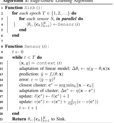
prediction at sensor Si. Algorithm 1 summarizes both the
local regression and quantization local learning at the edge network (note: η∈(0,1) is the learning rate used for both on-line K-means and SGD-based linear regression training).
Algorithm 1: Edge-centric Learning Algorithm
1 FunctionSink():
2 foreach epochT ∈ {1,2, . . .} do
3 foreach sensorSi in parallel do
4 hθi,{ck}Kk=1i ←Sensor(i) 5 end 6 end 7 8 FunctionSensor(i): 9 t←0 10 whilet < T do 11 (x, y) =context(t)
12 adaptation of linear model:∆θi←η(y−θix)x
13 prediction:yˆ=fi(θ,x)
14 error:e= (ˆy−y)2
15 closest cluster:c∗= arg minkkx−ckk
16 adaptation of cluster:∆c∗←η(x−c∗) 17 update:`(c∗)←`(c∗) + 1 18 update:e(c∗)←e(c∗) + 1 `(c∗)(e−e(c∗)) 19 t←t+ 1 20 end 21 Return θi,{ck}Kk=1 to Sink.
After receiving the trained linear models and the cor-respondingKclusters{θi,{ci,k}Kk=1,{`i,k}Kk=1,{ei,k}Kk=1}
from each sensorSi, the sink node has all the information
available to proceed with query analytics tasks, i.e., to answer to the regression queryq(x). By using these clusters, the sink chooses a subset of the functions {fi}ni=1 which
provide the lowest prediction error toq(x). The assumption is that the selected functions have seen plenty of training input vectors x similar to q(x) and, thus, should be able to predict the output yˆ more accurately. We propose two algorithms which define thiscloseness:
Distance Average (DA). In DA, we define closeness r
of function fi to the query q(x)as the Euclidean distance
between the query pointxof the regression queryq(x)and the closest clusterc∗i from the clusters set offi:
ri=kx−c∗ik. (2)
Reliable Average (RA). Initial experiments on the Beijing Air Quality dataset [17] demonstrated that some clusters c
are updated more frequently, which means they are very experienced while others are barely used. Hence, we define
closeness of the query q(x) to function fi by taking into
consideration the number`c∗
i and the prediction errore(c ∗
i)
of the closest clusterc∗
i to the query point x:
ri= 1 1 + exp−kx−c∗ ik + 1 1 + exp−e(c∗ i) + exp−`c∗i . (3)
A low distance kx−ck and a low error e are rewarded while a low number `c value is penalized. Note: `c and e are scaled in [0,1] for all the models in the sink.
Given a regression query q(x) issued to the sink, the closenessriis computed for each linear modelfi. The subset
of models F ⊂ {f1, . . . , fn} which are involved in the
predictionyˆ(answering) of the regression queryq(x)are the models with the top-Ccloseness values, withC=|F | ≤n. Then, the prediction yˆ derives from the average of the predictions yˆj = fj(x) : fj ∈ F, given the query q(x),
i.e., ˆ y= 1 C C X j=1 fj(x) :fj ∈ F. (4)
IV. PERFORMANCEEVALUATION
We evaluate the performance of our method with sensor networks which have power and computation limitations, thus, adopting machine learning models to greatly improve prediction accuracy and increase efficiency. We use the real air quality data-set [17] collected from air quality monitoring stations in Beijing to evaluate the prediction accuracy of our method. There are n = 36 independent sensors (IoT devices) transmitting knowledge to the sink, thus, we obtain
n = 36 different local regression models. In total there are 147,101 rows of data, such that on average there are approximately 4086 data elements for each sensor. We chose three contextual parameters from the dataset and verified that there was a correlation among them:x1 isPM25_AQI
and x2 is PM10_AQI. These parameters x = [x1, x2]
represent the concentration levels of fine particulate matter (air pollutant) with an aerodynamic diameter of less than 2.5, 1.0 respectively. We considery as the contextual parameter NO2_AQI, which represents the concentration levels of Nitrogen Dioxide. These gases are emitted by all combustion processes and have a negative impact on human life, example Nitrogen dioxide is linked with the summer smog [18]. Figure 3 shows the whole normalized dataset with a global linear regression plane over the context pairs(x, y).
We are assessing the prediction accuracy of our method-ology with the baseline and average solutions. Furthermore, we analyse the sensitivity of our model w.r.t. parameters:
C; number of models to average, andK; number of clusters per device while keeping number of epochsT = 100. In our comparative assessment we compare the methodologies:
• Baseline model (BL): all contextual pairs are
transmit-ted from all sensors to the sink and a single global regression model is trained.
Figure 3. 3D graph plot of the normalized context pairs(x, y)along with a linear regression plane.
Model Prediction error
BL 0.1152 I 0.1182 RA 0.1218 DA 0.1266 AVG 0.1284 Table I AVERAGERMSE.
Model Prediction error
BL 0.114 RA 0.1156 I 0.1176 DA 0.1208 AVG 0.128 Table II MINIMUMRMSE.
• Ideal model (I): Since this is a test scenario we know
from which sensorSieach test data is taken. Thus, the
learning modelfi is used to predict the result.
• Average model (AVG): All regression models are
aver-aged.
• Distance Averaging model (DA): The top-Cmodels are considered for regression w.r.t. the Euclidean distance-based closeness value are averaged in (4).
• Reliable Averaging (RA): The top-C models are con-sidered for regression w.r.t. closeness in (3) and aver-aged in (4).
To experiment with the hyper-parametersC andK, we ran the test scenario with the following rangesC∈ {1, . . . , n},
K∈ {1, . . . ,10}. The learning rate for both the on-line K-means and SGD linear regression was set toη= 0.01. Each combination was repeated 10 times and the result averaged to remove any bias. In each run, a random30%of the dataset was used for testing.
Tables I and II show the average and minimum prediction Root Mean Squared Error (RMSE) for each model, respec-tively. As expected, the BL model has the least error but it has to transmit the raw data at each step. Close behind it we find the I model, in which only the model from the device which owned the test data was used. This proves that, if we manage to create a mechanism thatperfectly guesseswhich is the probability distribution of the query pointx, we can approach this level of accuracy. In fact, AVG, which is an
0 5 10 15
0.12 0.13
Number of involved modelsC=|F |
RMSE BL I AVG DA(K= 1) DA(K= 2) DA(K= 5) DA(K= 10) RA(K= 1) RA(K= 2) RA(K= 5) RA(K= 10)
Figure 4. RMSE vs.Cfor variousK.
average over all the models, performs significantly worse than I model. When compared to the BL model, the RA model performs 50.2% better than the AVG model. This is attributed to the fact that we are taking into consideration the derived prediction errore(c∗)of the local model whose clusterc∗ is the closest to the incoming query pointxand not only dealing with the distance ofc∗ tox. Notably, we
obtain88.9%improvement in the minimum error (Table II) with RA when compared to the AVG model. We observe that the RA modelapproachesthe BL and I models.
Figure 4 shows the performance of the models in terms of RMSE against number of involved models C = |F |
for different K number of clusters per regression model. Overall, the worst performance by the RA and DA models is obtained withC = 1, i.e., we are taking only the top-1 model w.r.t. closeness value. This suggests that no matter how detailed our clusters are (i.e., a highK value), we still obtain a high RMSE since only one model is used. AsC
increases, we can observe that the models are more accurate, since more knowledge fromsimilarmodels is fused together. The RA model clearly outperforms the other models with
C ∈ {3,4,5} and even performs better than the I model. This indicates that RA successfully manages to learn the input data space by finding the most reliable regression models inF. However, asCincreases further, i.e.,C >10, thus involving more regression models in F, we inevitably gradually approach the AVG model, in which C = n. We found that the minimum RMSE for RA with K = 1 is achieved with C= 4, i.e., 11% of number of the models.
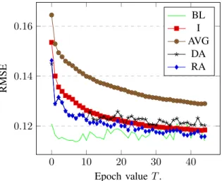
Figure 5 shows the RMSE against epoch T for all the models with K = 1 andC = 4. This setting corresponds to the best performance of the RA model. We can observe that from the first epoch, the DA and RA models are much more accurate than the AVG model. At the beginning since the clusters are fluctuating frequently (due to the on-line K-means algorithm), DA and RA perform very similarly. However, as sensors capture more context pairs, RA
out-0 10 20 30 40 0.12 0.14 0.16 Epoch value T. RMSE BL I AVG DA RA
Figure 5. RMSE vs. epochT withC= 4andK= 1.
0 10 20 30 40 0.12 0.14 0.16 Epoch value T. RMSE BL I AVG DA RA
Figure 6. RMSE vs. epochT withC= 1andK= 10.
performs DA due to the inclusion of the prediction error in the closeness value. This indicates that including more information in the clusters greatly improves our capability in understanding which regression models to select when averaging. The averaging function allows us to aggregate knowledge, which minimizes errors and gaps of knowledge, but at the same time we cannot aggregate all the knowledge together without any sense of the underlying data.
Figure 6 shows the RMSE against epoch T for all the models with K = 10andC = 1. This setting corresponds the worst performance of the RA model but still managed to surpass the AVG model. Since there is only one model selected, i.e.,C= 1, it heavily relies on picking the correct one; by selecting the wrong model, it incurs a huge penalty as there is no averaging in (4). At the beginning RA and DA models behave similarity w.r.t. RMSE, but eventually the RA model consistently manages to choose more appropriate regression models in F. On the other hand, the DA model is not able to pick the best model as it consistently performs
much worse than the AVG model. V. CONCLUSION
This paper focuses on leveraging the network edge with machine learning distributed over IoT sensing and comput-ing devices for improvcomput-ing prediction accuracy and com-munication efficiency. We propose two model variants (the DA and RA models) that successfully increase prediction accuracy by aggregating pieces of knowledge from similar local regression models derived from sensors. We introduce the concept of model closeness by adopting adaptive vector quantization of the input data space combined with regres-sion performance statistics.
Our future research agenda includes the applicability of the RA model variant in deep-learning tasks, especially when the contents of the federated contexts are not iden-tically distributed. Whilst we recognize that the proposed methodology can be further enhanced, this should serve as a reference point for further research in the field of collaborative machine learning in IoT environments.
ACKNOWLEDGMENT
This work was funded by the Erasmus+ Programme of the European Union under the PRIMES project (no. 2016-1-UK01-KA201-024631).
REFERENCES
[1] M. P. Durisic, Z. Tafa, G. Dimic, and V. Milutinovic, “A survey of military applications of wireless sensor networks,”
in2012 Mediterranean Conference on Embedded Computing
(MECO), pp. 196–199, June 2012.
[2] Y. Wang, S. Mao, and R. M. Nelms, “A distributed online algorithm for optimal real-time energy distribution in smart
grid,” in 2013 IEEE Global Communications Conference,
GLOBECOM 2013, Atlanta, GA, USA, December 9-13, 2013,
pp. 1644–1649, 2013.
[3] C. Anagnostopoulos, “Intelligent contextual information
col-lection in internet of things,”International Journal of Wireless
Information Networks, vol. 23, no. 1, pp. 28–39, 2016.
[4] C. Anagnostopoulos and S. Hadjiefthymiades, “Advanced principal component-based compression schemes for wireless
sensor networks,” ACM Trans. Sen. Netw., vol. 11, pp. 7:1–
7:34, July 2014.
[5] L. Bottou and Y. LeCun, “Large scale online learning.,” in
NIPS(S. Thrun, L. K. Saul, and B. Schlkopf, eds.), pp. 217–
224, MIT Press, 2003.
[6] C. Anagnostopoulos and P. Triantafillou, “Efficient scalable
accurate regression queries in in-dbms analytics,”IEEE
Inter-national Conference on Data Engineering (ICDE), February
2017.
[7] S. M. McConnell and D. B. Skillicorn, “A distributed
ap-proach for prediction in sensor networks,” inProc. SIAM Intl
[8] D. Tulone and S. Madden, “An energy-efficient querying framework in sensor networks for detecting node similarities,”
inProceedings of the 9th ACM International Symposium on
Modeling Analysis and Simulation of Wireless and Mobile
Systems, MSWiM ’06, (New York, NY, USA), pp. 191–300,
ACM, 2006.
[9] M. Satyanarayanan, P. Simoens, Y. Xiao, P. Pillai, Z. Chen, K. Ha, W. Hu, and B. Amos, “Edge analytics in the internet
of things,” IEEE Pervasive Computing, vol. 14, pp. 24–31,
Apr 2015.
[10] F. Bonomi, R. Milito, J. Zhu, and S. Addepalli, “Fog
com-puting and its role in the internet of things,” inProceedings
of the First Edition of the MCC Workshop on Mobile Cloud
Computing, MCC ’12, (New York, NY, USA), pp. 13–16,
ACM, 2012.
[11] M. Rabinovich, Z. Xiao, and A. Aggarwal, Computing on
the Edge: A Platform for Replicating Internet Applications,
pp. 57–77. Dordrecht: Springer Netherlands, 2004.
[12] H. Pang and K. Tan, “Authenticating query results in edge
computing,” in Proceedings of the 20th International
Con-ference on Data Engineering, ICDE ’04, (Washington, DC,
USA), pp. 560–, IEEE Computer Society, 2004.
[13] A. Manjeshwar and D. P. Agrawal, “Teen: A routing protocol
for enhanced efficiency in wireless sensor networks,” in in
Proc. IPDPS 2001 Workshops, 2001.
[14] K. Zeger and A. Bist, “Universal adaptive vector quanti-zation using codebook quantiquanti-zation with application to
im-age compression,” in[Proceedings] ICASSP-92: 1992 IEEE
International Conference on Acoustics, Speech, and Signal
Processing, vol. 3, pp. 381–384 vol.3, Mar 1992.
[15] L. Bottou, Large-Scale Machine Learning with Stochastic
Gradient Descent, pp. 177–186. Heidelberg: Physica-Verlag
HD, 2010.
[16] W. Barbakh and C. Fyfe, “Online clustering algorithms,”
International Journal of Neural Systems, vol. 18, no. 03,
pp. 185–194, 2008. PMID: 18595148.
[17] H. H. Y. Zheng, F. Liu, “U-air: When urban air quality
inference meets big data,” inProceedings of the 19th SIGKDD
conference on Knowledge Discovery and Data Mining, KDD
2013, August 2013.
[18] A. Richter, J. P. Burrows, H. Nusz, C. Granier, and U. Niemeier, “Increase in tropospheric nitrogen dioxide over
china observed from space,”Nature, vol. 437, pp. 129–132,