Forecasting Solar Flares Using Magnetogram-based Predictors and Machine Learning

Benvenuto, Federico, Bloomfield, Shaun and Georgoulis, Manolis (2018) Forecasting Solar

Flares Using Magnetogram-based Predictors and Machine Learning. Solar Physics, 293. p.

28. ISSN 0038-0938

Published by: Springer

URL: http://doi.org/10.1007/s11207-018-1250-4 <http://doi.org/10.1007/s11207-018-1250-4>

This version was downloaded from Northumbria Research Link:

http://nrl.northumbria.ac.uk/33146/

Northumbria University has developed Northumbria Research Link (NRL) to enable users to

access the University’s research output. Copyright

and moral rights for items on NRL are

retained by the individual author(s) and/or other copyright owners. Single copies of full items

can be reproduced, displayed or performed, and given to third parties in any format or

medium for personal research or study, educational, or not-for-profit purposes without prior

permission or charge, provided the authors, title and full bibliographic details are given, as

well as a hyperlink and/or URL to the original metadata page. The content must not be

changed in any way. Full items must not be sold commercially in any format or medium

without formal permission of the copyright holder. The full policy is available online:

http://nrl.northumbria.ac.uk/policies.html

This document may differ from the final, published version of the research and has been

made available online in accordance with publisher policies. To read and/or cite from the

published version of the research, please visit the publisher’s website (a subscription may be

required.)

arXiv:1801.05744v1 [astro-ph.SR] 17 Jan 2018

DOI: 10.1007/•••••-•••-•••-••••-•

Forecasting Solar Flares Using Magnetogram-based

Predictors and Machine Learning

Kostas Florios1,2 · Ioannis Kontogiannis1 · Sung-Hong Park3 ·Jordan A. Guerra3 · Federico Benvenuto4 ·D. Shaun Bloomfield5 ·Manolis K. Georgoulis1 c Springer••••

AbstractWe propose a forecasting approach for solar flares based on data from

Solar Cycle 24, taken by theHelioseismic and Magnetic Imager (HMI) on board theSolar Dynamics Observatory(SDO) mission. In particular, we use the Space-weather HMI Active Region Patches (SHARP) product that facilitates cut-out magnetograms of solar active regions (AR) in the Sun in near-realtime (NRT),

B

1 _{Research Center for Astronomy and Applied Mathematics, Academy of Athens,}

Greece

2 _{Department of Statistics, Athens University of Economics and Business, Greece} 3 _{School of Physics, Trinity College Dublin, Ireland}

4 _{Dipartimento di Matematica, Universit`a di Genova, Italy} 5 _{Northumbria University, Newcastle upon Tyne, NE1 8ST, UK}

taken over a five-year interval (2012 – 2016). Our approach utilizes a set of thir-teen predictors, which are not included in the SHARP metadata, extracted from line-of-sight and vector photospheric magnetograms. We exploit several Machine Learning (ML) and Conventional Statistics techniques to predict flares of peak magnitude>M1 and>C1, within a 24 h forecast window. The ML methods used are multi-layer perceptrons (MLP), support vector machines (SVM) and random forests (RF). We conclude that random forests could be the prediction technique of choice for our sample, with the second best method being multi-layer percep-trons, subject to an entropy objective function. A Monte Carlo simulation showed that the best performing method gives accuracy ACC=0.93(0.00), true skill statistic TSS=0.74(0.02) and Heidke skill score HSS=0.49(0.01) for >M1 flare prediction with probability threshold 15% and ACC=0.84(0.00), TSS=0.60(0.01) and HSS=0.59(0.01) for>C1 flare prediction with probability threshold 35%.

Keywords: Flares, Forecasting; Flares, Relation to Magnetic Field; Active

Regions, Magnetic Fields

1. Introduction

Solar flares are sudden brightenings that occur in the solar atmosphere and release enormous amounts of energy, over the entire electromagnetic spectrum. Flares are quite prominent in X-rays, UV, and optical lines (Fletcheret al.,2011) and they are often (but not always) accompanied by eruptions that eject solar coronal plasma into the interplanetary space (coronal mass ejections, CMEs). These very intense phenomena - the largest explosions in the solar system - are associated with regions of enhanced magnetic field, called active regions (AR) and are associated, in white light, with sunspot groups. Depending on their peak X-ray intensity, as recorded by the National Oceanic and Atmospheric Admin-istration’s (NOAA)Geostationary Operational Environmental Satellite(GOES) system, flares are categorized in classes, the strongest and most important being X, M and C (in decreasing order). Flare classification is logarithmic, with a base of 10, and is complemented by decimal sub-classes (e.g.M5.0, C3.2etc.).

The solar flare radiation may be detrimental to infrastructures, instruments and personnel in space, therefore flare forecasting is an integral part of con-temporary space-weather forecasting. Forecast mainly employs measurements of the AR magnetic field in the solar photosphere. Magnetic-field-based predictors represent AR magnetic complexity or the energy budget available to power flares. Recent developments in instrumentation have led to a regular production of such measurements offering the opportunity to produce extensive databases with properties suitable for solar flare prediction.

On the other hand, machine learning in recent years has become an increas-ingly popular approach for performing computer cognition tasks which were inherently possible only using human intelligence. Thus, machine learning (ML) is a subfield of artificial intelligence (AI) and it aims at using past data in order to train computers so that they can apply the accumulated knowledge to new, previously unseen, data. The acquisition of knowledge is the training phase and

the application of what was learned to future scenarios is the prediction phase. Typically, ML is more interested in prediction than conventional statistics. ML can also interface with conventional statistics in a field called statistical learning (Hastie, Tibshirani, and Friedman,2009). Learning is either called supervised or unsupervised depending on whether it is done with a teacher or not. Supervised learning comprises regression and classification, while unsupervised learning is also called clustering. In our study, we focus on classification, where a set of input variables or predictors belongs to one of two classes (binary classification). ML is more powerful than traditional statistical techniques such as, say, generalized linear models that include probit, logit, etc.for binary classification, because it can help model more complex nonlinear relationships. An introduction to ML research can be found in several textbooks (MacKay, 2003; Hastie, Tibshirani, and Friedman,2009).

Several researchers have recently used ML techniques to effectively forecast solar flares. More often, the techniques used by researchers were: neural networks (Wang et al., 2008; Yu et al., 2009; Colak and Qahwaji, 2009; Ahmed et al.,

2013), support vector machines (Li et al., 2008; Yuan et al., 2010; Bobra and Couvidat, 2015; Boucheron, Al-Ghraibah, and McAteer, 2015), ordinal logistic regression (Songet al.,2009), decision trees (Yuet al.,2009) and relevance vector machines (Al-Ghraibah, Boucheron, and McAteer,2015). Very recently, random forests have also been used (Barneset al.,2016; Liuet al.,2017).

We use predictors calculated from near-realtime (NRT) Space-weather HMI Active Region Patches (SHARP) data combined with state-of-the-art ML and statistical algorithms in order to effectively forecast flare events for an arbitrarily chosen 24-hour forecast window. Flare magnitudes of interest are>M1 and>C1. Prediction is binary, meaning that a given flare class is considered to either hap-pen or not within the next 24 hours after prediction. Our predictions are effective immediately, therefore with zero latency. Analysis involves a comprehensive NRT SHARP sample including all calendar days between years 2012 and 2016, at a cadence of 3 hours. Results in this work summarize the findings of the first eighteen months of the “Flare Likelihood And Region Eruption foreCASTing” (FLARECAST) project and, while based on ongoing work, we took every effort to present robust and unbiased results.

The contribution of the present work is twofold:

• The utilization of novel magnetogram-based predictors in a multi-parameter solar flare prediction model.

• The utilization of classic and novel ML techniques, such as multi-layer perceptrons (MLP), support vector machines (SVM) and especially, for one of the first times1_{, random forests (RF), for the forecasting of >M1}

and>C1 flares.

1_{In June 2017, we noticed a manuscript by Liuet al.(2017) which also uses the random forest}

algorithm for solar flare prediction using SDO/HMI data. Nevertheless, the specific details in that paper regarding the sampling strategy and the feature extraction are very different from our choices. For example, in Liuet al.(2017) only flaring ARs (at the level>B1 class) were considered and the sample size was N=845, while in our paper we consider both flaring and non-flaring ARs with N=23,134.

For the interested reader, the application code is available at http://dx.doi.org/

10.17632/4f6z2gf5d6.1, along with the benchmark dataset used in this work. The

run time for all methods is of the order of few minutes.

The analysis presented here is part of the EU Horizon 2020 FLARECAST project, aiming to develop a NRT online forecasting system for solar flares. The study is organized as follows: Section 2 describes the data selected to train and test the algorithms and presents the predictors used, together with background information on the solar physics aspects of magnetogram-based calculations. Section 3 describes the ML algorithms in terms of their core principles, along with some additional remarks and comments. Section 4 is devoted to the forecast experiments and a comparison with similar published results and statistics. Sec-tion 5 presents the main conclusions and future integraSec-tion of the present work in the FLARECAST operational system. Four Appendices, describing multiple complementary aspects of this work are also included.

2. Data and Classification Predictors

2.1. Data

The Helioseismic and Magnetic Imager (HMI; Scherrer et al., 2012) on board the Solar Dynamics Observatory (SDO; Pesnell, Thompson, and Chamberlin,

2012), provides regular full-disk solar observations of the three components of the photospheric magnetic field. The HMI team has created the Space Weather HMI Active Region Patches (SHARPs), which are cut-outs of solar regions-of-interest along with a set of parameters potentially useful for solar flare prediction (Bobraet al.,2014). For our analysis, we use the near-realtime (NRT), cylindrical equal area (CEA) SHARP data to calculate a set of predictors.

To associate SHARPs with flare occurrence we use the Geostationary Op-erational Environmental Satellite (GOES) soft X-ray measurements. For each SHARP we search for flares within the next 24 hours by either matching the NOAA AR numbers with those of the recorded flares or by comparing the corresponding longitude and latitude ranges, considering also the differential solar rotation.

The algorithms of Section3 are tested on a sample of the 2012-2016 SHARP dataset. We consider all days in the period October 1, 2012 to January 13, 2016 and for every given day we compute the set of predictors (see Section 2.2) at a cadence of 3 hours, starting at 00:00 UT. For our analysis, only SHARP cut-outs that correspond to NOAA ARs are considered. In this way, we get a fairly representative sample of the solar activity including several flares of interest, with a sufficiently high sampling frequency.

2.2. Predictors

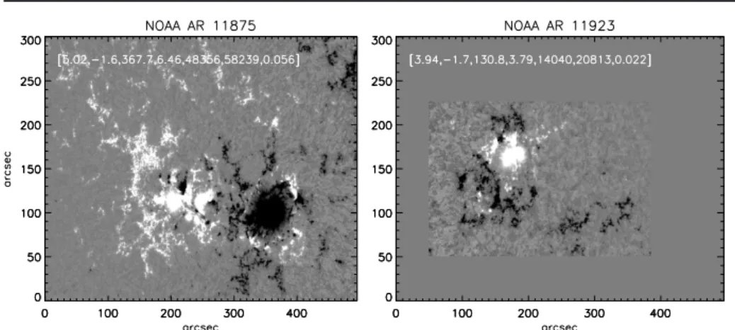
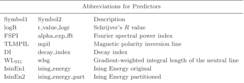
The set of thirteen predictors consists of both predictors already proposed in the literature and new ones, and comprises a subset of the parameter set de-veloped for the FLARECAST project. In Figure 1 we show two sample mag-netograms to demonstrate how the predictors reflect the complexity and size of

Figure 1. Two SHARP frames depicting AR with very different levels of flaring activity. NOAA AR 11875 (left) produced 7 C-, 0 M- and 0 X-class flares within 24h while NOAA AR 11923 (right) produced no flares. The two AR are scaled so as to retain their original relative size and, for comparison, vectors of the seven predictors used are included in the frames. The names of allK= 7 predictors [logR, FSPI, TLMPIL, DI, WLSG, IsinEn1, IsinEn2] are defined

in Section 2.2. High values of the predictors statistically indicate a powerful AR (left), with low values indicating a quiescent, flare-quiet AR (right).

the corresponding active region. The predictors utilized for this study are the following:

2.2.1. Magnetic Polarity Inversion Line (TLMPIL)

A magnetic polarity inversion line (MPIL) in the photosphere of an AR separates distinct patches of positive- and negative-polarity magnetic flux. Several studies have been carried out to investigate the relationship between flare occurrence and MPIL characteristics (Schrijver,2007; Falconeret al.,2012). We determine a specific subset of a MPIL, that has been also identified as MPIL*, with i) a strong gradient in the vertical component of the field across the MPIL and ii) a strong horizontal component of the field around the MPIL. MPIL* has been considered as the single most likely place in AR where potential magnetic instabilities, such as, say, magnetic flux cancellation and/or magnetic flux rope formation (Fang

et al., 2012) can take place. Such processes seem intimately related to flares. We use the total length Ltot of MPIL* segments in active regions as an MPIL

quantification parameter.

2.2.2. Decay Index (DI)

The decay index is a quantitative measure for the torus magnetic instability in a current-carrying magnetic flux rope (Kliem and T¨or¨ok,2006). It has been found that the larger the value of decay index in AR magnetic fields, the more likely it is to obtain a solar eruption involving a major solar flare (Zuccarello, Aulanier, and Gilchrist, 2015). We developed a decay index parameter derived by the ratio Lhs/hmin, where Lhs is the length of a highly sheared portion of

purported critical value of 1.5. This ratio can be used to measure the degree of instability in a flux rope. Notice that if there are more than one MPIL in an AR, then we calculate the ratio Lhs/hmin for every MPIL and take the peak value

for a given time, that represents the highest eruptive potential of the AR.

2.2.3. Gradient-weighted integral length of the neutral line(W LSG)

The gradient-weighted integral length of neutral line, WLSG, is defined in

Fal-coner, Moore, and Gary (2008) as,

WLSG=

Z

(∇Bz)dl , (1)

and corresponds to the line integral of the vertical-field (Bz) horizontal gradient

over all neutral line (or MPIL) segments on which the potential horizontal field is greater than 150 G. This MPIL-related property has been reported to show a useful empirical association with the occurrence of solar eruptions (flares, CMEs, SPEs; Falconeret al.,2011,2014) and is the main predictor used in the Magnetic Forecast (MAG4) forecasting service, developed in the University of Alabama

(http://www.uah.edu/cspar/research/mag4-page).

For these calculations of WLSG, two approximations of the vertical field Bz

are used:Blos(line of sight; uncorrected) andBr, keeping in mind that in former

case, only values for regions located within 30o _{from the central meridian are}

considered accurate. For each magnetogram, a MPIL mask is determined as in the calculation of MPIL characteristics, described previously. In order to select the strong-horizontal field segments of MPILs, the potential field extrapolation method developed by Alissandrakis (1981) is used. Finally, the horizontal gradi-ent ofBz is calculated numerically and integrated over all MPIL segments. The

accuracy of the calculated values was estimated by comparing flare rates derived from our calculations of WLSG (using Equation 4 along with Table 1 values in

Falconeret al., 2011) with the flare rates from the text output of MAG4.

2.2.4. Ising Energy (IsinEn1, IsinEn2)

The Ising energy is a quantity that parameterizes the magnetic complexity of an AR (Ahmedet al.,2010). For a two-dimensional distribution of positive and negative interacting magnetic elements, the Ising energy is defined as,

EIsing=−

X

ij

SiSj

d2 , (2)

whereSi(Sj) equals to +1 (-1) for positive (negative) pixels anddis the distance

between opposite polarity pairs. The interacting magnetic elements can be either the individual pixels with a minimum flux density value as in Ahmedet al.(2010) or the opposite-polarity partitions, produced using a flux-partitioning scheme (Barnes, Longcope, and Leka, 2005). The latter variation is introduced for the first time in the FLARECAST project, with promising results and an assessment

of its merit as a predictor is underway (Kontogiannis et al., in preparation). The Ising energy calculation produces four predictors, two for the line-of-sight magnetic field and two for the radial magnetic field component.

2.2.5. Fourier Spectral Power Index (FSPI)

The spectral power index, α, corresponds to the power-law exponent in fitting the one-dimensional power spectral densityE(k) extracted from magnetograms by the relation,

E(k)∼k−α_{. (3)}

This index parameterizes the power contained in magnetic structures of spa-tial scales l (= k−1_{) belonging to the inertial range of magnetohydrodynamic}

(MHD) turbulence. Empirically, AR with spectral power index higher than 5/3 (Kolmogorov’s exponent for turbulence) are thought to display an overall high productivity of flares (e.g.see Guerraet al.,2015).

The spectral power index has been historically calculated from the vertical component of the photospheric magnetic field, as inferred from the line-of-sight component assuming perfectly radial magnetic fields. First, the magnetogram is processed using the fast Fourier transform (FFT). A two-dimensional power spectral density (PSD) is then obtained as,

E(kx, ky) =|F F T[B(x, y)]|2. (4)

In order to express E(kx, ky) from the Fourier kx and ky to the isotropic

wavenumber k = (k2

x+ky2)1/2, it is necessary to calculate E(k)′ – the

inte-grated PSD over angular direction in Fourier space. From this last step, the one-dimensional PSD is obtained as E(k) = 2πkE(k)′_{. Finally, the power-law}

fit is performed as a linear fit in a logarithmic representation ofE(k)vs.k and

αis measured for the assumed turbulent inertial range of 2-20 Mm (i.e.0.05-0.5 Mm−1_).

2.2.6. Schrijver’s R value (logR)

The R-value property quantifies the unsigned photospheric magnetic flux near strong MPILs. The presence of such MPILs indicates that twisted magnetic structures carrying electrical currents have emerged into the AR through the solar surface. Therefore, R represents a proxy for the maximum free magnetic energy that is available for release in a flare. This property and its usefulness in forecasting was first investigated by Schrijver (2007).

The algorithm for calculating R is relatively simple, computationally inex-pensive, and was originally developed to use line-of-sight magnetograms from theMichelson Doppler Imager (MDI) (Scherreret al.,1995) on board theSolar and Heliospheric Observatory (SoHO). First, a bitmap is constructed for each polarity in a magnetogram, indicating where the magnitude of positive and negative magnetic flux densities exceeds the threshold value of±150 Mx cm−2_.

These bitmaps are then dilated by a square kernel of 3×3 pixels and the areas where the bitmaps overlap are defined as strong-field MPILs. This combined bitmap is then convolved with a Gaussian filter of full width at half maximum (FWHM)≈15 Mm. This particular value is constrained by how far from MPILs flares are observed to occur in extreme ultraviolet images of the solar corona. Finally, the convolved bitmap is multiplied by the absolute flux value of the line-of-sight magnetogram andRis calculated as the sum over all pixels. Notice that since theRvalue was implemented by Schrijver (2007) for MDI magnetograms, the SHARP magnetograms were resampled to the spatial scale of MDI, before the kernel application and subsequent calculations.

3. Machine Learning Algorithms and Conventional Statistics

Models

The ML algorithms used in this study are MLPs, SVMs and RFs. Among the hundreds of ML algorithms proposed for binary classification (e.g., Fern´ andez-Delgado et al., 2014) these three categories of algorithms are representative of three important approaches in ML: i) artificial neural networks (ANN), ii) kernel-based methods and iii) classification and regression trees. This is the reason why they were used in the present study, in order to furthermore investigate whether the usage of RFs could bring any improvements in flare prediction in comparison to SVMs and MLPs. The RFs belong to the category of ensemble methods while the MLPs utilize unconstrained optimization and SVMs use constrained optimization techniques (e.g., quadratic programming). In general, the working principle of ML comprises the following steps: i) train the model using a training set, ii) predict using the trained model and a testing set and iii) check whether the algorithm predicted well, in what is called the validation of the overal ML procedure. For further study, the reader is referred to Vapnik (1998), MacKay (2003) and Hastie, Tibshirani, and Friedman (2009).

3.1. Multi-Layer Perceptrons

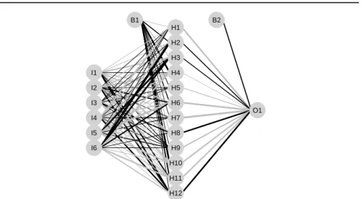
The MLP is a feed-forward network, thus it is described by the planar graph shown in Figure2. It contains an input layer, a hidden layer and an output layer of neurons. By the term neuron, we denote a basic processing unit where inputs are summed using specific weights and the result is squashed viaan activation function. The hidden layer might actually expand in a series of hidden layers. Nevertheless, the simplest MLP networks have just one hidden layer. In principle the term hidden describes every layer which is neither the input nor the output layer, but resides in between, as presented in Figure 2. A sufficient number of hidden nodes allows the MLP to approximate any continuous nonlinear function of several inputs with a desired degree of accuracy (Hornik, Stinchcombe, and White,1989), which is what characterizes the MLPs as universal approximators. It also holds that the greater the number of hidden nodes is, the more complex the nonlinear function that can be approximated by the neural network with a desired degree of accuracy. Usually, the number of hidden nodes does not have

I1 I2 I3 I4 I5 I6 H1 H2 H3 H4 H5 H6 H7 H8 H9 H10 H11 H12 O1 B1 B2

Figure 2. Example MLP neural network with 6 inputs, 12 hidden nodes, 1 output and 2 biases. Bold, darker lines indicate large positive weightsω.

to be more than twice the number of input nodes (or predictors). Actually, if too many hidden nodes are utilized, then the overfitting problem arises, which means that the MLP memorizes the sample observations and generalizes badly in the prediction phase. Usually, and in this study, the optimal number of hidden neurons (called size of the MLP) is determined with a fine-tuning procedure (e.g.

cross-validation approach, see Section4.2) before the training phase starts. The tuning phase is relatively time consuming, so it need not be executed every time the training starts. It can be conducted for a single realization of the training set.

An MLP network is actually a kind of a nonlinear regression (classification) technique, equivalent to a nonlinear mapping from input I to an output O =

O(I;ω, A). The output is a continuous function of the input and of the weights

ω. The network is described by a given architectureA, which typically defines the number of nodes in every layer (e.g.input, hidden and output). In general, MLP networks can be used to solve regression and classification problems. The statistical model of a MLP neural network for binary outcome, as described in the following, is based on MacKay (2003). For a recent survey on neural networks, the interested reader is referred to Prietoet al.(2016).

3.1.1. Classification Networks

We consider a MLP withlinputs calledIland biasB1. Also the network contains

a single hidden layer with jhidden nodesHj and biasB2. We have in generali

In the case of a classification problem, the propagation of the information from the inputsI to the outputO is described by,

α(1)j = L P l=1 ω_jl(1)Il+Bj(1); Hj=f(α(1)j ), α(2)i = J P j=1 ωij(2)Hj+Bi(2); Oi =g(α(2)i ), (5)

where, for example,f(α) = 1

(1+exp(−α)) andg(α) = 1 (1+exp(−α)).

The indexlis used for the inputsI1, . . . , IL, the indexjis used for the hidden

units and the indexi is used for the outputs (i= 1). The weightsωjl,ωij and

biases Bj, Bi define the parameter vector ω to be estimated. The nonlinear

logistic functionf at the hidden layer (also known as activation function) helps the neural network approximate any generic continuous nonlinear function with a desirable degree of accuracy (Hornik, Stinchcombe, and White,1989). Visually, a neural network can be represented as a series of layers consisting of nodes, where every node is connected to nodes of the subsequent layer only (feed forward networks).

In the case of binary classification, the MLP is trained using a dataset of examples D = {I(n),T(n)} by adjusting ω in order to minimize G(ω), the negative log-likelihood function,

G(ω) =−

N X

n=1

T(n)ln(O(I(n);ω)) + (1−T(n))ln(1−O(I(n);ω)). (6)

Notice that I(n) is the matrix of the predictors and T(n) is the vector of the targets for observation n = 1, . . . , N. In Equation 6, T(n) is 0 (1) for the negative (positive) class, respectively, andO(I(n);ω)is strictly between 0 and 1 (a probability) a fact that is ensured by Equations5.

3.2. Support Vector Machines

The SVM variant we use is theC-Support Vector Classification (C-SVC) accord-ing to the widely used library LIBSVM (Chang and Lin, 2011; Meyer, Leisch, and Hornik,2003).

Let us assume a vector of K predictor values at observation i, xi ∈ RK,

i= 1, . . . , N, which belongs in one of two classes, and an indicator vectory_∈RN

such that yi ∈ {1,−1}. Notice that the positive class has label +1 and the

negative class has label−1. Then theC-SVC solves the optimization problem: minimize 1₂ωTω+CPN i=1ξi, subject to yi(ωTφ(xi) +b)≥1−ξi, i= 1,2, . . . , N, ξi≥0, i= 1,2, . . . , N , (7)

where φ(xi) is an arbitrary unknown function which maps xi into a higher

dimensional space and C > 0 is the regularization parameter. The optimiza-tion in C-SVC model is performed by changing the decision variables: ω, b,

ξ. Actually, LIBSVM solves the dual of C-SVC which depends on a quantity:

K(xi,xj) =φ(xi)Tφ(xj), which is called thekernel function. While theφ(xi) is

unknown, the kernel function is known and is equal to the inner product ofφ(xi)

with itself but for different pairs of observations i and j. This is the so-called kernel trick of SVMs. As seen below, the kernel is a similarity measure and takes the maximum value of 1 when dist(xi,xj) = 0.

We have used the Radial Basis Function (RBF) (or Gaussian) kernel which is defined asK(x,x′_{) = exp(−γ||x−x}′_||2_{). A variant of theC-SVC model has}

been used for flare prediction in Bobra and Couvidat (2015).

For imbalanced datasets which account for rare events (e.g., in our case the >M1 flares) some researchers e.g. Bobra and Couvidat (2015) have used two different values for the regularization parameter C in Equation7, thereby penalizing more the constraint violations for the minority class. These authors have used C1 andC2 with a ratioC2/C1 ∈ {2,15}, whereC1 is the coefficient

for the majority class (no events) andC2is the coefficient for the minority class

(events). While we generally use the SVM in the original unweighted version in Equation 7, in auxiliary runs we experimented also with using different values

C1andC2with a ratioC2/C1∈ {2,15,20}to account for the imbalanced nature

of the>M1 flares dataset.

3.3. Random Forests

The RF is a relatively recent ML methodology, introduced by Breiman (2001). The RF approach is an ensemble of tree predictors, where we let each tree vote for the most popular class. It has been reported (Fern´andez-Delgadoet al.,2014) that RF offers significant performance improvement over other classification algorithms. The RF approach relies on randomness and involves the concept of split purity and the Gini index for variable selection (Breimanet al.,1984).

According to Hastie, Tibshirani, and Friedman (2009), the goal of the RF algorithm is to randomly build a set (or ensemble) of trees, by repeating the tree-formation process B times to create B trees. In particular, the algorithm: i) chooses a bootstrap sample from the training data, ii) grows a tree Tb to

the bootstrapped sample by applying consequently the following two substeps: Substep 1, select m variables randomly out of the M variables, and Substep 2, split the current node into two children nodes, having picked the best variable (node) from the m chosen ones. By repeating steps i) and ii) (where ii) consists of Substeps 1 – 2), the algorithm creates a set (called ensemble) of trees{Tb}B1.

Then, in the classification case studied in the present paper, a voting procedure for every treeTbis followed in order to obtain the class prediction of the random

forest.

This is one of the first times RF is used for flare forecasting. Other related works are Liuet al. (2017) and Barneset al. (2016). Furthermore, three recent applications of RF in astrophysics are by (Vilalta, Gupta, and Macri, 2013; Schuh, Angryk, and Martens,2015; Granett, 2017).

3.4. Implementation of ML algorithms

3.4.1. Multi-layer Perceptrons

MLPs were implemented using the R programming language and the nnet pack-age (Venables and Ripley, 2002). The options used were: linout=FALSE, to ensure that sigmoid activation functions are used at the output node, entropy = TRUE, to ensure that the negative log-likelihood objective function is minimized during the training phase (and not the default Sum of Squares Error (SSE) criterion), and size=iNode, where iNode for both>M1 flares and for>C1 flares was chosen with a tuning procedure.

3.4.2. Support Vector Machines

SVMs were implemented using the R programming language and the e1071 package (Meyer et al., 2015). The options used were: probability=TRUE, in order to obtain probability estimates for every element of the training set as well as probability estimates for every element of the testing set.

3.4.3. Random Forests

RFs were implemented using randomForest package (Liaw and Wiener,2002) in the R programming language. The options used were: importance = TRUE, to create importance information for every predictor, na.action=na.omit, to exclude records of predictors with missing values appearing in preliminary versions of the dataset (but lacking from the final version of the dataset).

3.5. Conventional Statistics Models

Non-ML (or statistical) methods also considered are: i) linear regression (LM), ii) probit regression (PR) and iii) logit regression (LG). Although multiple linear regression is known to be redundant for binary outcomes, since it can yield probabilistic predictions outside the interval [0,1], we still include it in the array of tested methods. The reason is that some practitioners still use it for binary outcomes (calling it linear probability model (LPM), see Greene (2002)) and there is always interest to consider ordinary least squares (OLS) as an entry-level method for any regression analysis. An interesting article about the lack of use of probit and logit in astrophysics modeling is de Souza et al. (2015). The statistical algorithms were implemented in the statistical programming language R using the lm and glm functions.

For a description of these well known methods the reader is referred to (Greene,2002; Winkelmann and Boes,2006).

4. Data preparation, Results and Discussion

First, we implement ML predictions on >M1 flares. Second, we use statistical methods for the prediction of >M1 flares. Third, we predict >C1 flares with

ML algorithms. Finally, we predict >C1 flares with the statistical algorithms. The following subsections describe these four experiments, presenting at first a single combination of training/testing set for every flare class and category of techniques.

Results are presented for the prediction step in terms of: i) skill scores profiles (SSP) of ACC, TSS and HSS as functions of the probability threshold, ii) ROC curves, and iii) RD plots for all methods: (for the explanation of metrics ACC, TSS, HSS as well as ROC curves and RD diagrams – see following Section4.3). Skill score profiles were created by a code we developed in R, ROC curves were created using the ROCR package (Sing et al., 2005), while reliability diagrams were created using the verification package (Laboratory,2015).

All algorithms were implemented and run using the R programming language 3.3.2 R Core Team (2016) and the RStudio 0.99 IDE.

4.1. Data Pre-processing

The data comprise the K = 7 predictors [logR, FSPI, TLMPIL, DI, WLSG,

IsinEn1, IsinEn2] described in Section 2.2 and computed using either the line-of-sight magnetograms,Blos, of SHARP data or the respective radial component,

Br (Bobra et al., 2014). Hence, we test K = 2×6 + 1 = 13 predictors2.

The sample comprises N = 23,134 observations, randomly split in half into

N1 = 11,567 observations for the training, and N2 = 11,567 observations for

the testing set. The random split is performed for 200 replications and all six prediction algorithms (i.e. MLP, SVM, RF, LM, probit and logit) of Section3 are trained and perform on identical training and test sets. The metrics ACC, TSS and HSS of Section4.3are computed always for the testing (out-of-sample) set. We have standardized all predictor variables to have mean equal to 0 and standard deviation equal to 1, because several ML algorithms involve non-linear optimization (e.g.MLPs). This helps to better train the ML algorithms and also explains the effect of every predictor variable on the studied outcome in the case of the statistical models LM, probit and logit.

4.2. Tuning of ML algorithms

As with any parameterized algorithm (e.g. simulated annealing, evolutionary algorithms, and other metaheuristics), the performance of ML algorithms de-pends on a number of crucial parameters which need to be fine tuned before the application of the ML procedure (e.g.training, testing and validation steps). The optimal tuning of ML algorithms is more or less still an open question in the ML community and always poses a big challenge for any practitioner. This choice of optimal options for the ML algorithms themselves is similar to the choice of optimal parameters for other numerical models, (e.g. MHD models), where the analyst also has to explore the optimal parameter space in several cru-cial parameters before conducting numerical MHD simulations. The algorithms

2 _{This is because, for predictor WL}

MLP, SVM and RF have their critical hyperparameters (e.g.parameters that are critical for the forecasting performance of every algorithm) tuned viaa 10-fold cross-validation study exploiting only the training set at one of its realizations. The set of plausible values for every ML algorithm is as follows: i) MLP: size (number of hidden neurons) ∈ {4,13,26} and decay (weight decay parameter)

∈ {10−3_,10−2_,10−1_{}, ii) SVM:γ (parameter in the RBF (or Gaussian) kernel)} ∈ {10−6_{, 10}−5_{, 10}−4_{, . . . , 10}−1

}and cost (regularization parameter)∈ {10,100}

and iii) RF: mtry (number of variables randomly sampled as candidates at each split)∈ {⌊√K⌋= 3}and ntree (number of trees to grow)∈ {500}.

Actually, we have tuned only the MLP and SVM classifiers, because the default RF values mtry=3 and ntree=500 immediately provided satisfactory results. Tuning of the MLP and SVM was mostly needed in the >M1 flares case, that was found harder to predict than>C1 flares, but was also performed in the >C1 flares case. Thus, the hyperparameters for MLP and SVM needed tuning since, for example, the default valuesγ= 1 and cost = 1 for SVM provided unsatisfactory results. We have used the tune.nnet and tune.svm functions of the R package e1071 for tuning the MLP and SVM, respectively. After the tuning, both MLP and SVM improved their performance significantly.

For the>M1 flares, the selected values are size = 26 and decay = 0.1 for the MLP andγ= 0.1 and cost = 10 for the SVM. These values are used throughout the remainder of this work. For the>C1 flares case, the selected values are size = 4 and decay = 0.1 for the MLP andγ = 0.001 and cost = 100 for the SVM.

4.3. Comparison Metrics

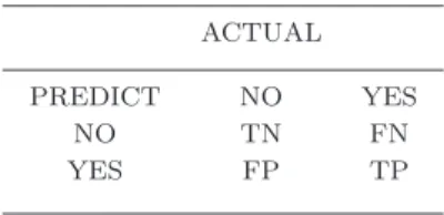
A wide variety of metrics exist in order to characterize the quality of binary classification. Among these, no single one is fit for all purposes. There exist two types of metrics, suitable for either categorical or probabilistic classification. In the former case a strict class membership is returned from the model and in the latter case a probability of membership is returned. In this section we concentrate on categorical forecast metrics for binary classification. In what follows, let ACC denote accuracy, TSS denote true skill statistic and HSS denote Heidke skill score. The performance of algorithms is measured using a number of metrics. These are derived from the so-called contingency table or confusion matrix, a representation of which is provided in Table1:

Table 1. 2×2 contingency table for binary forecasting

ACTUAL

PREDICT NO YES

NO TN FN

YES FP TP

Table 1 includes true positives (TP; events predicted and observed), true neg-atives (TN; events not predicted and not observed), false positives (FP; events

predicted but not observed) and false negatives (FN; events not predicted but observed), where N = TP + FP + FN + TN is the sample size. From these elements:

The meaning of ACC is the proportion correct, namely the number of correct forecasts of both event and non-event, normalized by the total sample size,

ACC = TP + TN

N . (8)

The TSS (Hanssen and Kuipers, 1965) compares the probability of detection (POD) to the probability of false detection (POFD),

TSS = POD−POFD = TP

TP + FN−

FP

FP + TN. (9)

Moreover, the TSS is the maximum vertical distance from the diagonal in the ROC curve, that relates the POD and POFD for different probability thresholds – see Section4. The TSS covers the range from−1 up to +1, while the value of zero indicates lack of skill. Values below zero are linked to forecasts behaving in a contrarian way, namely mixing the role of the positive class with the role of the negative class. In any negative TSS value, by exchanging the roles of YES and NO events, we can obtain the corresponding positive TSS value which would be identical in absolute value terms with the negative TSS value.

The HSS (Heidke, 1926) measures the fractional improvement of the forecast over the random forecast,

HSS = 2(TP×TN−FP×FN)

(TP + FN)(FN + TN) + (TP + FP)(FP + TN), (10)

which ranges from−∞to 1. Any negative value means that the random forecast is better, a zero value means that the method has no skill over the random forecast, and an ideal forecast method provides a HSS value equal to 1.

The TSS and HSS metrics are among the most popular metrics for comparison purposes in Meteorology and Space Weather and were conceptually compared in Bloomfield et al. (2012). In a probabilistic forecasting, such as the one for solar flares, they must be assigned a probability threshold, thus appearing as functions of this threshold.

To summarize, ACC is the most popular classification metric, but in rare events such as flares>M1, the ACC can be artificially high for the naive model which will always predict the majority class (“no event”). Thus, TSS and HSS are more suitable for flare prediction. Moreover, TSS has the advantage of being invariant to the frequency of events in a sample (e.g. see Bloomfield et al.,

2012). Typically, both TSS and HSS need to be evaluated, for a given probability threshold, in order to assess the merit of a given probabilistic forecasting model, such as the ones we develop in this study.

Regarding the probabilistic assessment of classifiers, the present study utilizes the visual approaches of Receiver Operating Characteristic (ROC) curves and

Reliability Diagrams (RD) (e.g.see Section4). The ROC describes the relation-ship between the POD and the POFD for different probability thresholds (e.g.

see Figure3b). The Area Under the Curve (AUC) in the ROC has an ideal value of one. The RD describes the relationship between the returned probabilities by the model and the actual observed frequencies of the data. A binning approach is used to construct the RD, in which probabilities are assigned to intervals of arbitrary length (for example we use 20 bins of length 0.05 each). For an example of RD, see Figure3c. Also, to algebraically assess the probabilistic performance of classifiers, we use the Brier Score (BS) (Brier, 1950) and Brier Skill Score (BSS) (Wilks,2011), as well as the AUC (Marzban,2004).

4.4. Results on >M1 Flare Prediction

4.4.1. Prediction of >M1 Flare Events Using Machine Learning

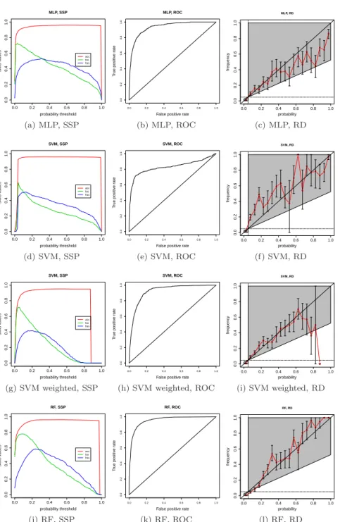
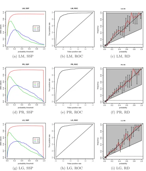
Figure3shows the forecast performances of the three tested ML methods, using both binary scores (SSP [left]; ROC [middle]) and probabilistic ones (RD [right]). In particular:

i) Regarding the MLPs, we notice a wide plateau with more-or-less flat profile for HSS and less so for TSS. This occurs because the number of hidden neurons (size=26) is twice the number of input neurons, causing the MLP to provide probability estimates clustered around 0 and 1. The ROC curve is reasonably good, with maximum TSS=0.726. Moreover, the RD shows a systematic over-prediction above a forecast probability of 0.4.

ii) For the SVMs, the SSP plateau noticed in case of the MLPs is not present here, with nearly monotonically decreasing values of TSS and HSS ap-pearing. The ROC curve shows a maximum TSS=0.629, while the RD seems slightly better than for MLP, with some under-prediction below a forecast probability of 0.4 and generally large uncertainties. When we use the weighted version of the SVM, with a ratio of C2/C1 = 20, then the

ROC curve improves providing a maximum TSS= 0.718, but the overall forecasting ability as measured by the SSP and RD remains worse than the MLP.

iii) With respect to the RFs, the SSP behaviour is such that HSS shows a plateau around its peak value, albeit smaller than in case of MLPs, while TSS monotonically decreases. This said, notice that the peak HSS and TSS values are higher in this case (e.g.TSS=0.780 and HSS=0.587). The ROC curve is better than that of MLPs and SVMs with a maximum TSS=0.780. The RD, finally, appears clearly better than those of MLPs and SVMs, presenting some mild under-prediction, mainly within error bars, above a forecast probability of 0.2.

4.4.2. Prediction of >M1 Flare Events Using Statistical Models.

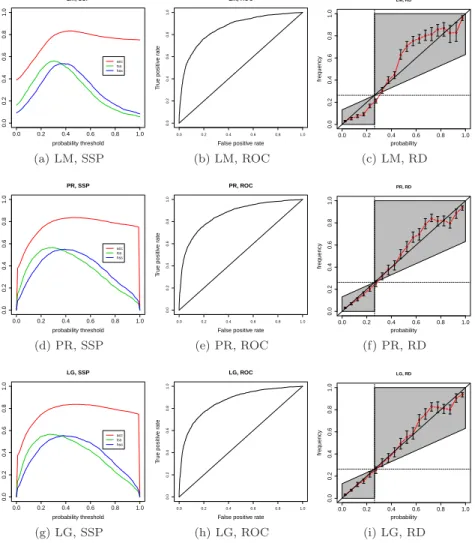
Figure4shows the forecast performances of the three tested statistical methods, for>M1 flare prediction. In particular:

Regarding the LM, the SSP is different between TSS and HSS, with TSS peaking more impulsively and for smaller probabilities and then decreasing nearly monotonically. The ROC curve shows also a significant performance with maximum TSS=0.744 that can also be seen in the RD, which shows a very good behavior, albeit with error bars, for the entire range of forecast probabilities.

As far as the PR is concerned, a slightly improved behavior in comparison with LM can be seen here, for the SSP, the ROC curves and the RD. The RD, also, seems more reliable in this case compared to LM, although differences are mostly within error bars.

For the LG, we notice a similar behavior as in the LM and especially PR method, and the RD in this case appears as good as the PR RD.

4.4.3. Monte Carlo Simulation for >M1 Flares

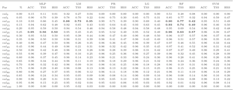
In Table2we provide the average values of the skill scores ACC, TSS and HSS for all prediction methods after the 200 replications of the Monte Carlo experiment regarding >M1 flares prediction. We notice from Table 2 that the maximum HSS=0.57 is obtained with the RF method for a probability threshold of 25%. The corresponding RF score values are ACC=0.96±0.00, TSS=0.63±0.02 and HSS=0.57±0.02. The second best method in Table 2 for the same probability threshold is MLP, with ACC=0.95±0.00, TSS=0.56±0.02 and HSS=0.50±0.02. Considering the threshold where the maximum TSS is observed, we get the optimal results for method RF and threshold 10%, with values ACC=0.90±0.00, TSS=0.77±0.01 and HSS=0.42±0.01. The second best method may be con-sidered the LM at 10% threshold with ACC=0.88±0.00, TSS=0.73±0.01 and HSS=0.35±0.01. The difference between RF and LM is statistically significant at 0.01% level as shown in Table4 at row 1. For the range of thresholds 10% to 25% the method RF yields increasing values of HSS and decreasing values of TSS. For example, an appealing forecasting model could be RF with threshold 15% and metrics ACC=0.93±0.00, TSS=0.74±0.02 and HSS=0.49±0.01 in Table2, but this would depend on the needs and requirements of a given decision maker.

0.0 0.2 0.4 0.6 0.8 1.0 0.0 0.2 0.4 0.6 0.8 1.0 MLP, SSP probability threshold skills v alues acc tss hss (a) MLP, SSP MLP, ROC

False positive rate

T rue positiv e r ate 0.0 0.2 0.4 0.6 0.8 1.0 0.0 0.2 0.4 0.6 0.8 1.0 (b) MLP, ROC 0.0 0.2 0.4 0.6 0.8 1.0 0.0 0.2 0.4 0.6 0.8 1.0 probability frequency MLP, RD (c) MLP, RD 0.0 0.2 0.4 0.6 0.8 1.0 0.0 0.2 0.4 0.6 0.8 1.0 SVM, SSP probability threshold skills v alues acc tss hss (d) SVM, SSP SVM, ROC

False positive rate

T rue positiv e r ate 0.0 0.2 0.4 0.6 0.8 1.0 0.0 0.2 0.4 0.6 0.8 1.0 (e) SVM, ROC 0.0 0.2 0.4 0.6 0.8 1.0 0.0 0.2 0.4 0.6 0.8 1.0 probability frequency SVM, RD (f) SVM, RD 0.0 0.2 0.4 0.6 0.8 1.0 0.0 0.2 0.4 0.6 0.8 1.0 SVM, SSP probability threshold skills v alues acc tss hss (g) SVM weighted, SSP SVM, ROC

False positive rate

T rue positiv e r ate 0.0 0.2 0.4 0.6 0.8 1.0 0.0 0.2 0.4 0.6 0.8 1.0 (h) SVM weighted, ROC 0.0 0.2 0.4 0.6 0.8 1.0 0.0 0.2 0.4 0.6 0.8 1.0 probability frequency SVM, RD (i) SVM weighted, RD 0.0 0.2 0.4 0.6 0.8 1.0 0.0 0.2 0.4 0.6 0.8 1.0 RF, SSP probability threshold skills v alues acc tss hss (j) RF, SSP RF, ROC

False positive rate

T rue positiv e r ate 0.0 0.2 0.4 0.6 0.8 1.0 0.0 0.2 0.4 0.6 0.8 1.0 (k) RF, ROC 0.0 0.2 0.4 0.6 0.8 1.0 0.0 0.2 0.4 0.6 0.8 1.0 probability frequency RF, RD (l) RF, RD

Figure 3. ML methods comparison for>M1 GOES flares prediction for (fromtoptobottom) MLP, SVM, weighted SVM and RF. From left toright we present the corresponding SSP, ROC and RD.

0.0 0.2 0.4 0.6 0.8 1.0 0.0 0.2 0.4 0.6 0.8 1.0 LM, SSP probability threshold skills v alues acc tss hss (a) LM, SSP LM, ROC

False positive rate

T rue positiv e r ate 0.0 0.2 0.4 0.6 0.8 1.0 0.0 0.2 0.4 0.6 0.8 1.0 (b) LM, ROC 0.0 0.2 0.4 0.6 0.8 1.0 0.0 0.2 0.4 0.6 0.8 1.0 probability frequency LM, RD (c) LM, RD 0.0 0.2 0.4 0.6 0.8 1.0 0.0 0.2 0.4 0.6 0.8 1.0 PR, SSP probability threshold skills v alues acc tss hss (d) PR, SSP PR, ROC

False positive rate

T rue positiv e r ate 0.0 0.2 0.4 0.6 0.8 1.0 0.0 0.2 0.4 0.6 0.8 1.0 (e) PR, ROC 0.0 0.2 0.4 0.6 0.8 1.0 0.0 0.2 0.4 0.6 0.8 1.0 probability frequency PR, RD (f) PR, RD 0.0 0.2 0.4 0.6 0.8 1.0 0.0 0.2 0.4 0.6 0.8 1.0 LG, SSP probability threshold skills v alues acc tss hss (g) LG, SSP LG, ROC

False positive rate

T rue positiv e r ate 0.0 0.2 0.4 0.6 0.8 1.0 0.0 0.2 0.4 0.6 0.8 1.0 (h) LG, ROC 0.0 0.2 0.4 0.6 0.8 1.0 0.0 0.2 0.4 0.6 0.8 1.0 probability frequency LG, RD (i) LG, RD

Figure 4. Same as Figure3, but for statistical methods: linear regression (LM;top), probit regression (PR;middle), and logit regression (LG;bottom).

4.5. Results on >C1 Flare Prediction

4.5.1. Prediction of >C1 Flare Events Using Machine Learning

We continue our computational experiments by training and performing our algorithms to the prediction of GOES >C1 flares. Figure 5 shows the forecast performances of the three tested ML methods, for >C1 flare prediction. In particular:

Regarding the MLP, we notice that since for the >C1 flares the number of hidden nodes selected is size=4, plateaus in HSS and TSS are not so eminent, contrary to the case of >M1 flare prediction. The ROC curve seems

satisfac-0.0 0.2 0.4 0.6 0.8 1.0 0.0 0.2 0.4 0.6 0.8 1.0 MLP, SSP probability threshold skills v alues acc tss hss (a) MLP, SSP MLP, ROC

False positive rate

T rue positiv e r ate 0.0 0.2 0.4 0.6 0.8 1.0 0.0 0.2 0.4 0.6 0.8 1.0 (b) MLP, ROC 0.0 0.2 0.4 0.6 0.8 1.0 0.0 0.2 0.4 0.6 0.8 1.0 probability frequency MLP, RD (c) MLP, RD 0.0 0.2 0.4 0.6 0.8 1.0 0.0 0.2 0.4 0.6 0.8 1.0 SVM, SSP probability threshold skills v alues acc tss hss (d) SVM, SSP SVM, ROC

False positive rate

T rue positiv e r ate 0.0 0.2 0.4 0.6 0.8 1.0 0.0 0.2 0.4 0.6 0.8 1.0 (e) SVM, ROC 0.0 0.2 0.4 0.6 0.8 1.0 0.0 0.2 0.4 0.6 0.8 1.0 probability frequency SVM, RD (f) SVM, RD 0.0 0.2 0.4 0.6 0.8 1.0 0.0 0.2 0.4 0.6 0.8 1.0 RF, SSP probability threshold skills v alues acc tss hss (g) RF, SSP RF, ROC

False positive rate

T rue positiv e r ate 0.0 0.2 0.4 0.6 0.8 1.0 0.0 0.2 0.4 0.6 0.8 1.0 (h) RF, ROC 0.0 0.2 0.4 0.6 0.8 1.0 0.0 0.2 0.4 0.6 0.8 1.0 probability frequency RF, RD (i) RF, RD

Figure 5. Same as Figure3, but for>C1 flare prediction.

tory with maximum TSS=0.574 and the RD is quite significant, showing no systematic over- or under-prediction.

With respect to the SVM, a purely monotonic decrease of TSS can be seen, following an instantaneous peak. Some plateau in HSS is also noticed, followed by a monotonic decrease. The ROC curve appears less satisfactory than in case of MLPs with maximum TSS=0.566 and the RD shows some systematic under-prediction for most of the forecast probabilities range.

For the RFs, one notices a relatively similar behavior with MLPs, albeit with a slightly more pronounced HSS peak. The ROC curve seems better behaved than in the previous two methods with maximum TSS=0.615 and the RD is arguably the best achieved together with the MLP RD.

4.5.2. Prediction of >C1 Flare Events Using Statistical Models

Figure6shows the forecast performances of the three tested statistical methods, for>C1 class flare prediction. In particular:

0.0 0.2 0.4 0.6 0.8 1.0 0.0 0.2 0.4 0.6 0.8 1.0 LM, SSP probability threshold skills v alues acc tss hss (a) LM, SSP LM, ROC

False positive rate

T rue positiv e r ate 0.0 0.2 0.4 0.6 0.8 1.0 0.0 0.2 0.4 0.6 0.8 1.0 (b) LM, ROC 0.0 0.2 0.4 0.6 0.8 1.0 0.0 0.2 0.4 0.6 0.8 1.0 probability frequency LM, RD (c) LM, RD 0.0 0.2 0.4 0.6 0.8 1.0 0.0 0.2 0.4 0.6 0.8 1.0 PR, SSP probability threshold skills v alues acc tss hss (d) PR, SSP PR, ROC

False positive rate

T rue positiv e r ate 0.0 0.2 0.4 0.6 0.8 1.0 0.0 0.2 0.4 0.6 0.8 1.0 (e) PR, ROC 0.0 0.2 0.4 0.6 0.8 1.0 0.0 0.2 0.4 0.6 0.8 1.0 probability frequency PR, RD (f) PR, RD 0.0 0.2 0.4 0.6 0.8 1.0 0.0 0.2 0.4 0.6 0.8 1.0 LG, SSP probability threshold skills v alues acc tss hss (g) LG, SSP LG, ROC

False positive rate

T rue positiv e r ate 0.0 0.2 0.4 0.6 0.8 1.0 0.0 0.2 0.4 0.6 0.8 1.0 (h) LG, ROC 0.0 0.2 0.4 0.6 0.8 1.0 0.0 0.2 0.4 0.6 0.8 1.0 probability frequency LG, RD (i) LG, RD

Figure 6. Same as Figure4, but for>C1 flare prediction.

For the LM, we notice a decrease in the ACC of the method and some more-or-less similar behavior in the behaviour of HSS and TSS. The ROC curve seems satisfactory with maximum TSS=0.562, while the RD appears to show a systematic over-prediction below a forecast probability of 0.4 and a systematic under-prediction above a forecast probability of 0.4 (excluding probabilities >

0.9).

Regarding the PR, similar behaviour with LM appears for the SSPs, while the ROC curve seems slightly better with maximum TSS=0.566. The RD curve shows some systematic under-prediction, although generally within error bars.

Finally, for the LG, one notices a similar behaviour in the SSP, as in the case of LM and PR, but arguably a better behaved ROC curve with maximum TSS=0.567. The RD seems to bee the best behaved, compared to those of LM and PR.

4.5.3. Monte Carlo Simulation for >C1 Flares

In Table3we provide the average values of the skill scores ACC, TSS and HSS for all prediction methods after the 200 replications of the Monte Carlo experiment regarding >C1 flares prediction. We notice from Table 3 that the maximum HSS=0.60 is obtained with the RF method for a probability threshold of 40%. The corresponding skill score values are ACC=0.85±0.00, TSS=0.59±0.01 and HSS=0.60±0.01. The second best method in Table 3 for the same probability threshold is obtained with the LG method, with ACC=0.83±0.00, TSS = 0.54±

0.01 and HSS=0.56±0.01. Considering again the probability threshold where the maximum TSS is observed, we get the optimal results for the RF method and threshold 30% with values ACC=0.82±0.00, TSS=0.61±0.01 and HSS = 0.57±

0.01. The second best method may be considered the MLP (or the LG in a tie) at 30% threshold with ACC=0.81±0.00, TSS=0.57±0.01 and HSS=0.53±0.01. For a range of probability thresholds (30% – 40%) the method RF yields increasing values of HSS and decreasing values of TSS. As a result, again it is not clear which is the optimal value of the threshold probability, if we choose to simultaneously optimize both TSS and HSS. For example, an appealing RF forecasting model is with threshold 35% and skill scores ACC=0.84±0.00, TSS=0.60±0.01 and HSS=0.59±0.01 in Table3. These results are generally above those reported for

>C1 class flares predictability, namely TSS∈[0.50,0.55] and HSS ∈[0.40,0.45] (Al-Ghraibah, Boucheron, and McAteer, 2015; Boucheron, Al-Ghraibah, and McAteer, 2015). In brief, we believe that our data samples, both training and testing, are comprehensive and generally unbiased.

4.6. Assessment of Prediction Methods and Predictor Strength

Following the presentation of results in Tables 2 and 3, we can see that both for>M1 and>C1 flare prediction, RF delivers the best skill score metrics for a wide range of probability thresholds. The second best method is MLP together with LG. In this setting we perform some additional evaluation that confirms these results.

Regarding the predictors strength, we present analytical results in Appendix A. It seems that logR and WLSGrank in the first places both for>C1 and>M1

flare prediction, closely followed by the Ising energy and the TLMPIL.

In order to investigate the robustness of our results, we present additional results in Appendix C where we make predictions once a day (at 00:00 UT). The mean evolution (over 200 Monte Carlo iterations) of ACC, TSS and HSS with respect to the probability threshold is presented. Likewise, the BS, AUC and BSS are presented. The main finding is that issuing forecasts once a day keeps similar average skill scores with issuing forecasts eight times a day, but the associated uncertainties (e.g.standard deviations) are higher in the case of daily predictions.

A final word for the comparison of ML algorithmsvs.conventional statistics models for this specific dataset and positive/negative class definitions is provided in Appendix D. There, we have included auxiliary meta-analysis of the results in Tables 2and3 in order to clearly show whether the ML category of prediction algorithms does any better than the conventional statistics models in the >M1 and>C1 flare prediction cases. A multicriteria analysis using the weighted-sum (WS) method (Greco, Figueira, and Ehrgott,2016) seems appropriate in order to aggregate the performance metrics ACC, TSS and HSS of all classifiers as a func-tion of the probability threshold (e.g.using equal weights for the aggregation). In this way, a composite index (CI), as a measure of overall utility, is computed for every algorithm and probability threshold combination. There exist 21×6 = 126 such alternatives when we use a 5% probability threshold grid, such as the grid in Tables2and3. The ranking, in non-increasing order, of the CI reveals the overall merit of every probabilistic classifier and also allows us to draw conclusions for groups of classifiers, such as the group of ML methods (comprising RF, SVM and MLP) and the group of conventional statistics methods (comprising LM, PR and LG). Appendix D presents this multicriteria WS analysis, revealing that overall, in>C1 flare prediction ML outperforms conventional statistics methods by 71%vs.29% in the synthesis of the top 100(1/6) = 16.6% performing methods (top 21 methods out of total 126 ones). Likewise, in the >M1 flare prediction case, ML outperforms conventional statistics methods by 62% vs. 38% in the synthesis of the top 100(1/6) = 16.6% performing methods. So, it seems that

>C1 flare prediction is more advantageous for ML versus statistical methods, in comparison to the>M1 flare case. This is due to the low performance of the SVM in>M1 flare prediction, which is due to the way we have implemented, for simplicity, the SVM for a highly unbalanced sample in >M1 flare prediction3_,

using a singleCconstant and not two differentC1, C2constants during the SVM

training with Equation7.

In auxiliary runs (available upon request), we also noticed that when the sample size is very low, using ML algorithms poses no advantage over conven-tional statistics models. In order to have proper training, the ML algorithms

needN >2,000 forK= 13, especially for the>M1 flare prediction.

4.7. Statistical Tests for Random Forestvs. MLP and Calculation of

AUC and Brier Skill Scores

In Section 4.7.1we present results of a t-test between the two best performing methods according to maximizer thresholds for either TSS or HSS for >M1 class and >C1 class flares cases. Section 4.7.2 presents additional calculations reporting on BS, BSS and AUC, used for assesing classification in the prediction.

3_{Even by using the SVM weighted variant and recomputing the WS ranking using this variant,}

4.7.1. Unpaired t-tests to Compare Two Means for TSSandHSS of Random Forest vs. MLP

A t-test compares the means of two groups. Here, we use thet-test to compare the mean TSS (respectively HSS) of the RF methodvs.those of the MLP method (or in general the second best performing method). Means are considered with respect to the Monte Carlo simulations performed on the 200 replications of the previous section. The TSS- (respectively HSS-) values considered are those for specific probability thresholds maximizing either TSS or HSS. Table4 presents thet-test results regarding the best and the second best methods with respect to either TSS or HSS for these specific probability thresholds.

We find that RF is always (i.e.8/8 of times) statistically better than the second best method (which is the MLP 4/8 of times), with respect to both TSS and HSS.

4.7.2. Calculation of AUC and Brier Skill Scores

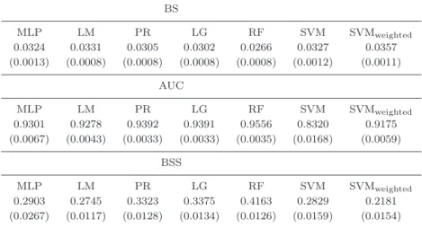
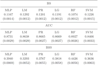
Tables5and6present the calculated mean values of BS, AUC and BSS for the

>M1 and>C1 flare prediction cases, respectively.

For the >M1 flare case (Table5), results show that, on average, the best BS and BSS results are achieved with the RF method (BS = 0.0266; BSS=0.4163). The best AUC results are achieved with the RF method (AUC = 0.9556), but also PR (AUC=0.9392) and LG (AUC=0.9391) methods.

For the>C1 flare case (Table 6), results show that, on average, the best BS and BSS results are achieved with the RF method (BS=0.1074; BSS=0.4426). The best AUC results are also achieved with the RF method (AUC=0.8927), with other methods (except SVM) following closely. The SVM probably needs better fine-tuning, given its sensitivity onγ and cost (see Section4.2).

re ca st in g S o la r F la re s U si n g M a ch in e L ea rn in g

Table 2. Monte-Carlo scenario 1, based on 200 SHARP datasets, on>M1 GOES flare prediction. Numbers in boldface correspond to the most significant results of a given method (MLP: multi-layer perceptron; LM: linear regression; PR: probit regression; LG: logit regression; RF: random forest; SVM: support vector machine).

MLP LM PR LG RF SVM

Par % ACC TSS HSS ACC TSS HSS ACC TSS HSS ACC TSS HSS ACC TSS HSS ACC TSS HSS

val₀ 0.00 0.15 0.11 0.01 0.32 0.27 0.04 0.00 0.00 0.00 0.00 0.00 0.00 0.51 0.48 0.08 0.00 0.00 0.00 val_{5 0.05 0.90 0.70 0.39 0.78 0.70 0.22 0.84 0.75 0.30 0.85 0.75 0.31 0.85 0.77 0.32 0.94 0.59 0.47} val₁₀ 0.10 0.93 0.66 0.45 0.88 0.73 0.35 0.90 0.71 0.39 0.90 0.69 0.40 0.90 0.77 0.42 0.95 0.51 0.49 val_{15 0.15 0.94 0.62 0.48 0.92 0.65 0.43 0.93 0.64 0.45 0.93 0.63 0.45} 0.93 0.74 0.49 _{0.96 0.46 0.50} val₂₀ 0.20 0.95 0.59 0.50 0.94 0.54 0.46 0.94 0.58 0.48 0.94 0.58 0.48 0.95 0.69 0.54 0.96 0.42 0.48 val_{25 0.25} 0.95 0.56 0.50 0.95 0.45 0.45 0.95 0.52 0.49 0.95 0.52 0.49 0.96 0.63 0.57 0.96 0.39 0.47 val_{30 0.30 0.95 0.53 0.50 0.95 0.38 0.44 0.96 0.47 0.49 0.96 0.48 0.50 0.96 0.57 0.57 0.96 0.37 0.46} val_{35 0.35 0.96 0.50 0.50 0.96 0.31 0.39 0.96 0.41 0.47 0.96 0.43 0.49 0.96 0.51 0.57 0.96 0.35 0.45} val_{40 0.40 0.96 0.47 0.50 0.96 0.26 0.35 0.96 0.36 0.45 0.96 0.39 0.47 0.97 0.46 0.55 0.96 0.33 0.44} val₄₅ 0.45 0.96 0.44 0.49 0.96 0.21 0.31 0.96 0.32 0.42 0.96 0.35 0.45 0.97 0.41 0.52 0.96 0.31 0.42 val_{50 0.50 0.96 0.42 0.48 0.96 0.18 0.28 0.96 0.28 0.39 0.96 0.31 0.42 0.97 0.37 0.49 0.96 0.29 0.41} val₅₅ 0.55 0.96 0.39 0.47 0.96 0.16 0.25 0.96 0.25 0.36 0.96 0.27 0.39 0.96 0.32 0.45 0.96 0.28 0.39 val_{60 0.60 0.96 0.37 0.45 0.96 0.14 0.23 0.96 0.21 0.33 0.96 0.24 0.36 0.96 0.28 0.41 0.96 0.26 0.38} val₆₅ 0.65 0.96 0.34 0.44 0.96 0.11 0.19 0.96 0.18 0.29 0.96 0.21 0.32 0.96 0.24 0.36 0.96 0.24 0.36 val_{70 0.70 0.96 0.32 0.42 0.96 0.09 0.16 0.96 0.16 0.25 0.96 0.18 0.28 0.96 0.19 0.31 0.96 0.22 0.34} val₇₅ 0.75 0.96 0.29 0.40 0.96 0.08 0.13 0.96 0.13 0.22 0.96 0.15 0.25 0.96 0.15 0.25 0.96 0.21 0.32 val₈₀ 0.80 0.96 0.27 0.37 0.95 0.06 0.12 0.96 0.11 0.18 0.96 0.12 0.21 0.96 0.11 0.19 0.96 0.18 0.29 val_{85 0.85 0.96 0.24 0.34 0.95 0.05 0.09 0.96 0.08 0.14 0.96 0.09 0.16 0.96 0.08 0.14 0.96 0.16 0.26} val₉₀ 0.90 0.96 0.20 0.31 0.95 0.03 0.06 0.95 0.05 0.10 0.95 0.06 0.10 0.95 0.04 0.08 0.96 0.13 0.22 val_{95 0.95 0.96 0.15 0.25 0.95 0.02 0.04 0.95 0.03 0.06 0.95 0.03 0.05 0.92 0.01 0.02 0.96 0.08 0.14} val₁₀₀ 1.00 0.00 0.00 0.00 0.95 0.02 0.03 0.00 0.00 0.00 0.00 0.00 0.00 0.00 0.00 0.00 0.00 0.00 0.00 S O L A : K F _ e t _ a l _ 1 4 _ 0 1 _ 2 0 1 8 . t e x ; 1 8 J a n u a r y 2 0 1 8 ; 1 :

K

.

F

significant results of a given method (MLP: multi-layer perceptron; LM: linear regression; PR: probit regression; LG: logit regression; RF: random forest; SVM: support vector machine).

MLP LM PR LG RF SVM

Par % ACC TSS HSS ACC TSS HSS ACC TSS HSS ACC TSS HSS ACC TSS HSS ACC TSS HSS

val₀ 0.00 0.00 0.00 0.00 0.39 0.16 0.09 0.00 0.00 0.00 0.00 0.00 0.00 0.28 0.03 0.01 0.00 0.00 0.00 val_{5 0.05 0.52 0.33 0.21 0.44 0.23 0.14 0.47 0.27 0.17 0.48 0.28 0.17 0.52 0.34 0.21 0.29 0.03 0.02} val₁₀ 0.10 0.66 0.49 0.35 0.51 0.32 0.20 0.58 0.40 0.27 0.60 0.42 0.29 0.64 0.48 0.34 0.44 0.22 0.13 val_{15 0.15 0.72 0.55 0.43 0.58 0.40 0.27 0.66 0.49 0.36 0.68 0.50 0.38 0.71 0.55 0.42 0.75 0.54 0.45} val₂₀ 0.20 0.76 0.57 0.48 0.66 0.48 0.35 0.73 0.55 0.44 0.74 0.55 0.45 0.76 0.59 0.48 0.80 0.57 0.53 val_{25 0.25 0.79 0.57 0.51 0.74 0.55 0.45 0.78 0.56 0.49 0.78 0.57 0.50 0.79 0.61 0.53 0.82 0.56 0.55} val_{30 0.30} 0.81 0.57 0.53 _{0.79 0.57 0.51 0.80 0.57 0.53} 0.81 0.57 0.53 0.82 0.61 0.57 _{0.83 0.54 0.55} val_{35 0.35 0.82 0.56 0.55 0.82 0.55 0.54 0.82 0.56 0.55 0.82 0.56 0.55} 0.84 0.60 0.59 0.84 0.52 0.55 val_{40 0.40 0.83 0.55 0.55 0.83 0.52 0.54 0.83 0.53 0.55} 0.83 0.54 0.56 0.85 0.59 0.60 _{0.84 0.50 0.54} val₄₅ 0.45 0.84 0.53 0.55 0.83 0.47 0.52 0.84 0.50 0.55 0.84 0.51 0.55 0.85 0.56 0.59 0.84 0.48 0.53 val_{50 0.50 0.84 0.50 0.55 0.83 0.40 0.47 0.84 0.47 0.53 0.84 0.48 0.53 0.85 0.54 0.59 0.84 0.46 0.52} val₅₅ 0.55 0.84 0.48 0.53 0.81 0.34 0.41 0.83 0.43 0.50 0.84 0.45 0.52 0.85 0.51 0.57 0.83 0.44 0.51 val_{60 0.60 0.84 0.45 0.51 0.80 0.28 0.35 0.82 0.38 0.46 0.83 0.41 0.48 0.85 0.48 0.55 0.83 0.42 0.49} val₆₅ 0.65 0.83 0.41 0.49 0.79 0.22 0.29 0.82 0.34 0.42 0.82 0.37 0.44 0.84 0.44 0.52 0.83 0.38 0.46 val_{70 0.70 0.82 0.37 0.45 0.78 0.18 0.24 0.81 0.29 0.37 0.81 0.32 0.40 0.83 0.40 0.48 0.82 0.35 0.43} val₇₅ 0.75 0.82 0.33 0.41 0.77 0.15 0.20 0.80 0.25 0.32 0.80 0.27 0.35 0.82 0.34 0.43 0.81 0.32 0.39 val₈₀ 0.80 0.81 0.28 0.36 0.77 0.12 0.17 0.79 0.20 0.27 0.79 0.22 0.29 0.81 0.28 0.36 0.81 0.28 0.36 val_{85 0.85 0.79 0.22 0.29 0.76 0.10 0.14 0.78 0.16 0.22 0.78 0.18 0.24 0.79 0.21 0.29 0.80 0.24 0.31} val₉₀ 0.90 0.78 0.16 0.21 0.76 0.08 0.11 0.77 0.13 0.18 0.77 0.14 0.19 0.78 0.15 0.21 0.79 0.19 0.25 val_{95 0.95 0.75 0.08 0.11 0.76 0.07 0.10 0.76 0.09 0.13 0.76 0.09 0.13 0.76 0.08 0.12 0.77 0.14 0.19} val₁₀₀ 1.00 0.00 0.00 0.00 0.75 0.06 0.08 0.00 0.00 0.00 0.00 0.00 0.00 0.00 0.00 0.00 0.00 0.00 0.00 S O L A : K F _ e t _ a l _ 1 4 _ 0 1 _ 2 0 1 8 . t e x ; 1 8 J a n u a r y 2 0 1 8 ;

Table 4. Unpaired t-tests to compare the means of TSS and HSS metrics (out-of-sample) for the best and the second best methods in

>M1 and>C1 flare forecasting.

>M1 class flares prediction

No. Metric Threshold (%) Best Second Best p-value

1 TSS 10 RF LM <10−4

2 HSS 10 RF LM <10−4

3 TSS 25 RF MLP <10−4

4 HSS 25 RF MLP <10−4

>C1 class flares prediction

No. Metric Threshold (%) Best Second Best p-value

5 TSS 30 RF MLP <10−4

6 HSS 30 RF MLP <10−4

7 TSS 40 RF LG <10−4

8 HSS 40 RF LG <10−4

Table 5. Mean values for BS, BSS and AUC for all tested models on the prediction

of>M1 flares. Means are obtained after 200 Monte-Carlo replications. Parentheses

underneath values denote standard deviations. Notice that smaller values indicate better performance for BS, whereas higher values indicate better performance for AUC and BSS. BS MLP LM PR LG RF SVM SVMweighted 0.0324 0.0331 0.0305 0.0302 0.0266 0.0327 0.0357 (0.0013) (0.0008) (0.0008) (0.0008) (0.0008) (0.0012) (0.0011) AUC MLP LM PR LG RF SVM SVMweighted 0.9301 0.9278 0.9392 0.9391 0.9556 0.8320 0.9175 (0.0067) (0.0043) (0.0033) (0.0033) (0.0035) (0.0168) (0.0059) BSS MLP LM PR LG RF SVM SVMweighted 0.2903 0.2745 0.3323 0.3375 0.4163 0.2829 0.2181 (0.0267) (0.0117) (0.0128) (0.0134) (0.0126) (0.0159) (0.0154)