A study of the Exponentiated Gradient +/- algorithm for stochastic optimization of neural networks

(1)

UC Santa Cruz

UC Santa Cruz Electronic Theses and Dissertations

Title

Permalink

https://escholarship.org/uc/item/4ck5k544

Author

Parks, David Freeman

Publication Date

2019

Peer reviewed|Thesis/dissertation

(2)

UNIVERSITY OF CALIFORNIA SANTA CRUZ

A study of the Exponentiated Gradient +/- algorithm for stochastic optimization of neural networks

A thesis submitted in partial satisfaction of the requirements for the degree of

MASTER OF SCIENCE in COMPUTER SCIENCE by David F. Parks September 2019

The Thesis of David F. Parks is approved:

Professor Manfred K. Warmuth

Professor Shawfeng Dong

Professor J. Xavier Prochaska

Quentin Williams

(3)

(4)

List of Figures

1.1 SGD vs. Momentum . . . 6 1.2 Momentum vs. Nesterov . . . 7 1.3 Nesterov vs. Adagrad . . . 9 1.4 Adagrad vs. Adadelta . . . 11 1.5 Adadelta Initialization . . . 16 1.6 Adadelta vs. WidnowGrad . . . 17 1.7 Adadelta vs. RMSProp . . . 18 1.8 RMSProp vs. Adam . . . 19 2.1 EG vs. SGD convergence . . . 24 2.2 UScaling convergence . . . 26

2.3 Visualization of normalization methods . . . 27

2.4 RMSPRop vs. EG . . . 34

3.1 Choosing a U parameter . . . 37

3.2 U scaling parameter experiment . . . 38

3.3 Weights distribution of EG±vs. Nesterov . . . 39

3.4 Biases distribution of EG±vs. Nesterov . . . 39

3.5 EG±Unnormalized . . . 40

3.6 50% random noise experiment . . . 41

3.7 10k features of random Gaussian noise experiment. . . 42

(7)

3.9 EG with adaptive learning rate . . . 47

3.10 EG with L1 regularization experiment . . . 49

3.11 Weight sharing applied to EG± . . . 50

3.12 Weight sharing experiment detailed plot. . . 51

3.13 Comparing EG±to SGD with L2 regularization. . . 52

3.14 CNN results on CIFAR10 dataset . . . 54

3.15 Activation values of EG±vs. Nesterov . . . 54

(8)

List of Tables

3.1 Comparing trainers on MNIST, displaying test set accuracy over time. Rows are per number of samples trained on, columns are per optimization algorithm. . . 44

3.2 Comparing all gradient optimization methods on a 2 layer MNIST dataset, including EG±with adaptive learning rate from Adadelta, the adaptive EG± uses a global learning rate parameter of 0.02, U=40, andρ=0.95. . . 46

3.3 EG vs other optimizers compared using a 32 layer residual net-work on the cifar10 dataset. . . 55

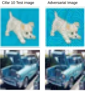
3.4 Comparison of EG optimizer with varying normalization method against other optimizers using 1000 test cifar10 samples and ad-versarial versions of the same images. . . 58

(9)

Abstract

A study of the Exponentiated Gradient +/- algorithm for stochastic optimization of neural networks

by David F. PARKS

Exponentiated Gradient +/- (abbr. EG±) is a gradient update algorithm drawn from work by Manfred Warmuth (Kivinen and Warmuth, 1997) in the online learning setting. This thesis ports the algorithm into the context of deep neural networks and analyses its fitness in that context compared to the current state of the art gradient update methods. Existing methods employ an additive update scheme whereby some fraction of the gradient is added to the weight values to update them at each iteration in the gradient descent algorithm. EG± provides a multiplicative update scheme whereby a proportion of the gradient is multiplied into the original weight value, and then normalized to update the weight. EG±is motivated by using a relative entropy regularization. This thesis analyzes various properties and experimental results of the algorithm in com-parison to other update methods, and analyzes EG±in the context of state of the art residual networks and challenging vision problems. Three published imple-mentations are experimented with, and demonstrate that EG±performs better than SGD when there are many noisy features, and that it compares well with commonly used state-of-the art gradient descent optimization methods. EG± also performs better than most SGD based optimizers on black-box adversarial attacks, with the exception of non momentum based SGD with which it per-forms similarly.

(10)

Acknowledgements

Foremost, I would like to thank Professor Manfred Warmuth for overseeing this work and providing guidance, inspiration, and for introducing me to many tal-ented experts in the field from across the globe. I also want especially mention Professor Shawfeng Dong who both mentored me in aspects of optimization theory as well as advised me on multiple projects involving implementations of neural networks on multiple frameworks, and in cluster computing with neural networks. The experience gained in my work with Professor Dong has bene-fited this work in innumerable ways. I would like to thank Professor J. Xavier Prochaska from Astronomy for supporting work I’ve done in applying neural networks to problems in the Astronomy domain, which has provided me with a much deeper intuition and understanding of the algorithms applied in this the-sis. I would like to thank Professor Ram Akella, and Dr. Jay Pujara, whom I’ve learned from and worked on related research projects, all of whom have pro-vided me tremendous amounts of information that went directly into this work and all of whom have helped with research projects that directly affected my knowledge in this topic area. I would like to thank Ryan Hausen, a fellow grad-uate student with whom I’ve often collaborated with and bounced uncountably many ideas off of since starting this work.

(11)

Chapter 1

Introduction

This thesis will introduce the Exponentiated Gradient ± (EG±) algorithm in Chapter2as an alternative gradient descent optimization method. In Chapter

3we will explore the properties of EG± and compare the algorithm to 8 of the most commonly used optimization algorithms used in neural network training today. The core conclusions we derive are that EG±performs or or near state of the art on common datasets such as MNIST and CIFAR10; it performs well on simple fully connected networks as well as the more complex architectures of residual networks (ResNet); it performs better with features consisting of ran-dom noise than modern optimizers; and EG±shares beneficial properties with vanilla SGD (stochastic gradient descent) on black box adversarial attacks that other optimizers perform poorly on.

Before introducing EG± let’s take a tour through the existing, gradient de-scent optimizers, starting with vanilla SGD.

1.1 Stochastic Gradient Descent Optimization

Stochastic Gradient descent is the workhorse algorithm for training artificial neural networks today. Stochastic gradient descent (SGD) is the most basic

(12)

method in a family of gradient descent update algorithms. SGD is a simple, effi-cient, and effective algorithm for updating the weights of the network given the gradient. The update rule for SGD is simply:wt+1 =wt−η∇wJ(wt), wherew

is a vector of weights (the networks trainable weights and biases for each layer, and other trainable weights such asγandβused in batch normalization),tis the training iteration of the algorithm, andη is the learning rate, a (typically small) step size which is specified as a hyper-parameter of the algorithm, J is a loss function that evaluates the fitness of the network for a set of weights. Given the gradient of the loss function with respect to the weights SGD takes a fraction of the gradient and subtracts it from the weights, taking a linearly approximated step in the direction of the negative gradient.

A single update step in SGD can be applied using a gradient computed over (a) one sample of the data (stochastic gradient descent), (b) a mini-batch of uni-formly random samples (mini-batch gradient descent), or (c) the entire data set (full batch gradient descent). For notational brevity this document always as-sumes updates are taken with respect to a mini-batch of samples, as is typical in practice.

A number of variants of SGD have been developed that provide improve-ments to the basic SGD algorithm. These algorithms add concepts such as mo-mentum, per-weight learning rates, and other beneficial features. The family of commonly used gradient descent optimization algorithms is discussed in the following sections.

1.2 Gradient descent algorithm variants

We will start by reviewing the most popular optimization methods (Ruder,2016;

Pascanu et al.,2013) employed by today’s neural network frameworks. For each of the update algorithms there will be a visualization of how the algorithm deals

(13)

with a prototypical problem in optimization, which is exemplified by a plateau-ing in one dimensionx1, and a steep gradient in another dimensionx2. Schaul et al.(2013) propose this among a number of unit tests to assess the suitability of an update algorithm.

The following gradient update algorithms are all implemented by the major frameworks such as Tensorflow, Torch, Caffe, etc.

• SGD (Stochastic Gradient descent)— The original and most basic form of gradient based optimization methods.

• SGD with Momentum— Adds a momentum term that alleviates the zig-zag problem of SGD.

• Nesterov— Performs momentum updates more intelligently.

• Adagrad— Incorporates per-weight learning rate which decays over time.

• Adadelta— Ameliorates the decaying learning rate of Adagrad while main-taining per-weight learning rates.

• Window Grad— This method was published as “idea 1” with Adadelta and restricts the time period over which we accumulate the gradients to a window.

• RMSProp— Another variant on Adagrad, similar to Adadelta which com-putes a per-weight learning rate, with some benefits over Adadelta.

• Adam— Applies concepts of both momentum and adaptive weights while correcting for initialization bias.

Notable among these algorithms is that they all employ an additive update method just as SGD does. In SGD,wt+1 = wt−η∇wJ(wt) , a fraction of the

(14)

negative gradient is added to the previous weights. To contrast that, a multi-plicative update method multiplies each weight by an exponential factor that has the ith component of the negative gradient in the exponent. In practice this has the effect of being a relatively small number slightly above or below one which gets multiplied into the existing weight in the update process. The family of exponentiated gradient optimization algorithms fall under this second paradigm, which we we will introduce in Chapter2, and study in Chapter3.

Assuming the reader is familiar with stochastic gradient descent, let’s look at each of SGD’s variants in turn with a visualization of each algorithm optimizing a 2D prototypical example. Each of these algorithms have been re-implemented for this project in Matlab to produce these visualizations.

1.2.1 Vanilla SGD

In vanilla SGD, gradient descent updates are performed by:

wt+1=wt−η∇wJ(wt) (1.1)

∇_wJ the gradient of the weights with respect to the loss function. This is the gradient calculated by backprop.

η is a scalar learning rate provided to the algorithm as a hyperparameter.

w is a vector of all network weights.

t is a scalar time step, representing the iteration comprising a forward pass for making a prediction, and a backward pass to compute the gradients.

SGD performs its update by taking a linear step in the direction of the nega-tive gradient and then recomputing the weights and gradient at that point.

1.2.2 SGD with Momentum

The first addition to vanilla SGD is adding a momentum term (Qian,1999). The momentum term is akin to the speed gained by a ball rolling downhill. At the

(15)

top of the hill the ball starts rolling slowly, building up momentum as it con-tinues downhill. It will reach a maximum terminal velocity depending on the medium it’s traveling through (air for example). This has a particularly ben-eficial effect when traveling down a valley (Sutton,1986). When the gradient surface provides a path towards a better optimum in one direction, but a steep gradient in other directions SGD is known to oscillate, slowing progress towards the objective. The momentum term minimizes progress along the axis of oscilla-tion, and increases momentum along the axis where the gradient doesn’t change.

The SGD update with momentum is given by the equations:

vt+1=γvt+η∇wJ(wt) (1.2)

wt+1 =wt−vt+1 (1.3)

∇wJ the gradient of the weights with respect to the loss function. This is the

gradient calculated by backprop.

v a vector of computed velocity terms per each weightw.

t is a scalar time step, representing the iteration comprising a forward pass for making a prediction, and a backward pass to compute the gradients. In Figure1.1 the oscillation effect of SGD (in red) is quite visible, whereas momentum draws a path that appears much more "natural".

1.2.3 Nesterov accelerated gradient descent

Nesterov accelerated gradient descent (Nesterov,1983) makes a small, but ben-eficial change to the concept of momentum. Nesterov updates take the momen-tum of the previous update into account before computing the gradient, then upon computing the gradient takes a "correction" step. Whereas momentum

(16)

FIGURE1.1: Momentum updates in yellow, vanilla SGD in red. SGD can oscillate back and forth in a valley, but momentum of-fers a smoothing effect that draws it out of the oscillation pattern.

simply takes a step in the gradient direction. This can be thought of essentially as a reordering of the optimization process where momentum is calculated first before taking a step and then intelligently correcting for any error that occurred. On convex problems Nesterov’s approach has provably better bounds than SGD with Momentum. However the theoretical guarantees are imperfect in the face of stochastic gradient noise due to mini batches of samples not contain-ing a perfect gradient. This is discussed in more detail in Sutskever’s thesis (Sutskever,2013).

In the non convex setting, there are no theoretical guarantees about how Nes-terov will perform, however this, update-then-correct strategy has been demon-strated to perform more stably in a wide variety of cases.

(17)

FIGURE1.2: Momentum update in red, Nesterov update in yel-low. Nesterov updates take momentum from the previous step into account prior to deciding where to compute the gradient, then computes the gradient and takes a “corrected” gradient step, smoothing out the progression and still avoiding SGD’s

os-cillation.

The Nesterov accelerated gradient update is given by the equations:

vt+1 =γvt+η∇wJ(wt−γvt) (1.4)

wt+1=wt−vt+1 (1.5)

v a vector of computed velocity terms per each weightw.

(18)

1.2.4 Adagrad

Adagrad (Duchi et al.,2011) aims to improve on gradient descent by effectively adjusting the learning rate per weight based on the history of the gradients for that weight. To accomplish this adagrad accumulates the square of the gradient each time-step, and divides the current gradient by the square root of previous sum of square gradients. This has the beneficial effect of normalizing the learn-ing rate based on the past values. Weights with small gradients will have their effect boosted compared to weights with large gradients. This is particularly important in deep neural networks where early layers will be more significantly impacted by the vanishing gradient problem (Bengio et al.,1994;Pascanu et al.,

2013). The downside of Adagrad is that the accumulation of the square gradient in the denominator causes the learning rate to decay over time. This is often cited as a problem, though it can be noted that a simple heuristic solution to that problem would be to increase the global learning rate passed as a parameter to the algorithm.

The Adagrad update is given by the following equations, first describing the non-vectorized form (since Adagrad uses per-weight updates), and then the vectorized form:

gt,i=∇wJ(wt,i) (1.6)

wt+1,i=wt,i−η·gt,i (1.7)

wt+1,i=wt,i− η p Gt,ii+ ·gt,i (1.8) wt+1=wt− η √ Gt+ gt (1.9)

gt,i the per-weight gradient w.r.t. the loss function.

wt,i each trainable weight in the network indexed byiat time stept.

(19)

FIGURE 1.3: Adagrad update shown in yellow, compared with the Nestrov update in red.

Gt ∈Rd×d, wheredis the number of weights inw, is a diagonal matrix where

the diagonal elements indexed byi, iare the sum of the square gradients with respect toθiup to time stept.

Gt,ii is one of the diagonal elements ofG.

is a small value to avoid numerical issues.

is the Hadamard product, a.k.a. element-wise vector multiplication.

1.2.5 Adadelta

Adadelta Zeiler(2012) attempts to take the best of Adagrad while eliminating the decaying learning rate. Adadelta does this by allowing the accumulated square gradient term to decay over time, taking only a fraction of the accumula-tor on each step, which causes the estimate to be biased towards recent updates over earlier updates. Adadelta further maintains a sum of square weight values.

(20)

Taking the ratio between decaying square weight values and decaying square gradient values provides a learning rate per weight that adjusts to be smaller for gradients that are large and larger for gradients that are small.

This has a dual benefit of helping train weights that are making slow progress, and keeping them in line, relatively speaking, with weights that have a larger gradient. This also has benefit in that it naturally increases the learning rate in earlier layers where the vanishing gradient problem will be more pronounced (Bengio et al.,1994;Pascanu et al.,2013).

The Adadelta update is given by the following equations:

wt+1 =wt+ ∆wt (1.10) ∆wt=− RM S[∆w]t−1 RM S[g]t gt (1.11) RM S[w]t= p E[∆w2_] t+ (1.12) RM S[g]t= p E[g2_] t+ (1.13) E[g2]t=γE[g2]t−1+ (1−γ)g2t (1.14)

γ is a hyperparameter configured similarly to Momentum with a common default of 0.9.

η is a scalar learning rate provided to the algorithm as a hyperparameter. E[g2]_t is the running average at time stept,Eis only a running approximation to

Eexpectation.

g is the vector of gradients.

g2 is the element-wise square of the gradientsg.

is the Hadamard product, a.k.a. element-wise vector multiplication. is a small value to avoid numerical issues.

(21)

FIGURE 1.4: Adagrad in red compared to Adadelta in yellow. Adadelta is initialized with the gradient sums = 1.0 at start to

avoid pathological initialization issues.

1.2.5.1 Adadelta Initialization Issues

Adadelta has a few issues that are identified here. The initialization of the gra-dient sums is quite critical. The algorithm can be pathologically slow when the gradient sum is initialized to zero. An initialization of 1.0 seems to be rea-sonable, producing convergence that seems reasonable in the toy example used here. However initializing to a large number such as 10.0 causes the algorithm to exhibit the same zig-zag effect of vanilla stochastic gradient descent, in fact it will converge so slowly as to be irrelevant. Even after 1000 iterations the zig-zag effect remains when the gradient sums are in this poor state. It should be further noted that the zig-zag effect in thex1dimension doesn’t affect progress in thex2

(22)

The issues with initialization are particularly important because we experi-ment with using adadelta’s per-weight learning rate in our exponentiated gra-dient update algorithms (see section3.7). The initialization issues are visualized in Figure1.5.

In summary, Adadelta allows us to eliminate the per-weight learning rate, though the algorithm exhibits pathological states under certain conditions. It’s hard to know whether these issues are commonly encountered in practice.

1.2.6 Window Grad

Window Grad (Zeiler, 2012) was proposed in the same paper with Adadelta. It’s not as widely implemented as Adadelta or other methods. Window Grad leaves out an accumulator of the change in weight values and only utilizes an exponentially decaying accumulation of the gradients. Whereas Adadelta com-pletely eliminates the learning rate, and adjusts the weights to their hypothetical unit value, Window Grad can be thought of as an update in the units of the gra-dient. Window Grad requires a learning rate to be set. Adadelta can be thought of as the completed extension of the Window Grad idea. Visualization in1.6.

The Windowgrad update is given by the following equations:

wt+1=wt+ ∆wt (1.15) ∆wt=− η RM S[g]t gt (1.16) RM S[g]t= p E[g2_] t+ (1.17) E[g2]t=γE[g2]t−1+ (1−γ)gt2 (1.18)

(23)

E[g2]_t is the running average at time stept,Eis only a running approximation to

Eexpectation.

is the Hadamard product, a.k.a. element-wise vector multiplication. is a small value to avoid numerical issues.

1.2.7 RMSprop

RMSprop (Hinton) is an unpublished algorithm proposed by Hinton. Ironically the citation commonly used for it is to slide 29 lecture 6 from a lecture by Hinton. RMSprop can be compared very similarly to Adadelta. It attempts to extend Adagrad in a very similar way that Adadelta does. It maintains the per-weight learning rate while eliminating the decaying learning rate inherent in Adagrad.

RMSprop maintains a "cache" of past weight values which decay over time given a decay parameter and accumulates the square gradient. The current gra-dient is divided by this "leaky" cache to modulate the learning rate per weight. RMSprop maintains a global learning rate parameter that Adadelta gets rid of.

One notable difference that is apparent based on the visualizations provided in this thesis (Figure 1.7) is that RMSprop does not have the same initializa-tion problem that Adadelta has. The visual here shows Adadelta and RMSprop performing almost identically, however it needs to be noted that Adadelta was initialized with a good initial state (1’s for the gradient sum).

(24)

The RMSprop update is given by the following equations: wt+1 =wt− η p E[g2_] t+ ·gt (1.19) E[g2]t=γE[g2]t−1+ (1−γ)g2t (1.20)

η is a scalar learning rate provided to the algorithm as a hyperparameter. E[g2]_t is the running average at time stept,Eis only a running approximation to

Eexpectation.

t is a scalar time step, representing the iteration comprising a forward pass for making a prediction, and a backward pass to compute the gradients. is a small value to avoid numerical issues.

1.2.8 Adam

Adam (Kingma and Ba,2014) is another adaptive optimization method which applies a momentum term in a new way. Adam is often cited as the best all around stochastic optimization method to start with. Adam applies the concept of momentum as well as adaptive learning rates per weight. Adam operates in much the same way as RMSprop in that it maintains a history of square gradi-ents that it uses to adapt the per-weight learning rate. Adam further accounts for the fact that the initialization causes a bias towards zero and accounts for this by computing the first and second moments correcting for the bias. Adam updates are visualized in Figure1.8.

(25)

The Adam update is given by the following equations: wt+1=wt− η √ ˆ vt+ ·mˆt (1.21) ˆ mt= mt 1−β1 (1.22) ˆ vt= vt 1−β2 (1.23) mt=β1mt−1+ (1−β1)gt (1.24) vt=β2vt−1+ (1−β2)g2t (1.25)

m an exponentially decaying average of past gradients

ˆ

m the bias-corrected first moment

v an exponentially decaying average of past gradients squared

ˆ

v the bias-corrected second moment

β1 a hyperparameter with a recommended default of 0.9

β2 a hyperparameter with a recommended default of 0.999

t is a scalar time step, representing the iteration comprising a forward pass for making a prediction, and a backward pass to compute the gradients. η is a scalar learning rate provided to the algorithm as a hyperparameter.

(26)

FIGURE1.5: Adadelta progress using 4 different initializations of the gradient sum. In red the gradient sum is initialized to 0.0, which is the default implementation of Adadelta by the papers author in ConvnetJS. This initialization has a pathological issue in this 2D example causing convergence to be extremely slow due to a slowly accumulatingx2sum, and quickly accumulating dient sum. In yellow and blue Adadelta is initialized with a gra-dient sum of 0.1 and 1.0, both reasonable initializations which converge to within 0.1 of the x2 axis in 25 steps and 6 steps respectively. The green line initializes the gradient sum with 5.0 and converges within 41 steps while exhibiting SGD’s oscillation back and forth in the valley. Higher initialization values

(27)

FIGURE 1.6: Adadelta in red vs. Window Grad in yellow, ini-tialized with a "good" sum-square gradient initialization of 1.0 to

(28)

FIGURE1.7: In red, Adadelta with a gradient sum initialization of 1’s (e.g. a “good” initialization), and RMSprop in yellow. Both perform very similarly on this 2 dimensional example, and long term convergence is quite similar: Both converge on thex dimen-sion in 6 steps, though after 100 iterations RMSprop had moved down to -100 in the y direction, vs. -300 for Adagrad, so Adagrad

(29)

FIGURE1.8: RMSprop shown in red with Adam updates shown in yellow. Although the RMS prop visualization appears to be-have better in this case, the true test of an optimizer in high di-mensional space is how well it performs on test set evaluation. Low dimensional visuals can help in understanding the behav-ior, but are not necessarily a clear indicator of optimal

(30)

Chapter 2

Exponentiated Gradient

±

Update Algorithm

In this Chapter we introduce the Exponentiated Gradient ±(henceforth EG±) (Kivinen and Warmuth, 1995, 1997) algorithm, and its predecessor the Expo-nentiated Gradient algorithm (henceforth EG). EG was introduced by Manfred Warmuth and Jyrki Kivinen in 1995 in the context of linear online predictors. The algorithm has been introduced for use in neural networks formally by Srini-vasan et al.(2002), for which we extend the analysis to a more modern context, and informally discussed inLangford(2007).

EG± generalizes the Exponentiated Gradient (EG) algorithm which main-tains a probability distribution over weights. EG does not allow for weights to change from positive to negative or vice versa. EG± operates by doubling the number of weights and performs an EG update to both positive and negative components of the weight.

(31)

2.0.1 Exponentiated Gradient

The Exponentiated Gradient (EG) algorithm performs an update by computing a multiplicative factor for each weight and multiplying that factor into each indi-vidual weight, then re-normalizing by dividing by the total sum of the weights. A global learning rate parameter that is used to scale the update factor, and functions the same as it does with SGD and its variants.

The Exponentiated Gradient algorithm is derived by trading off the relative entropy with the loss ameliorated by the learning rate that is defined by the fol-lowing minimization problem: wt+1 = argmin

ws.t.P wi=1 P wiln_ww_t,ii +ηJ(w) and

this results in the update algorithm given below. EG is motivated by using a relative entropy regularization.

wt+1,i = wt,i·e(−η∇wJ(wt+1,i)) PN j=1wt,j ·e(−η∇wJ(wt+1,j)) ≈ wt,i·e (−η∇wJ(wt,i)) PN j=1wt,j·e(−η∇wJ(wt+1,j)) (2.1)

wt,i is a single weight at time steptindexed byi.

wt,j is a single weight at time steptindexed byj.

N number of weights inw

i i∈1, ..., N, per each weight inw

j j∈1, ..., N, per each weight inw

2.0.2 Exponentiated Gradient±

EG± is a generalization of the Exponentiated Gradient (EG) algorithm which allows weights to take on positive or negative values. EG± achieves this by

(32)

maintaining two weight vectors,w+ ={x ∈_Rd_|_x _≥₀_}_and_w− ₌_{_x _∈

Rd|x≥ 0}, wheredis the number of weights in the neural network, represented byw=

{x ∈ _Rd_}_{. The basic EG update is applied to the each weight vector separately,}

then scaled by aU parameter, and normalized. The neural network weights take on the valuew=w+−w−.

EG± shares some properties with SGD, Figure 2.1 demonstrates a simple plot where EG± and SGD perform the same updates given a fixed gradient as the weight value updates from 0.1to −0.1. In later sections we will visualize this (Figure2.4) and show comparable performance on adversarial samples in Section3.14.

(33)

The EG±update is given by the equations: w+_t+1,i=U · w + t,ir+t,i PN j=1w + t,jr + t,j+w − t,jr − t,j (2.2) w−_t+1,i=U · w − t,ir − t,i PN j=1w + t,jr + t,j+w − t,jr − t,j (2.3) where

r+_t,i= exp −η∇wt,iJ(wt,i)

(2.4) r−_t,i = exp η∇_w_t,iJ(wt,i)

= 1

r+_t,i (2.5)

U U is a scaling parameter that is provided as a hyperparameter, typical val-ues are 20 to 80.

wt,i A single EG±weight at update stept, indexed byi.

wt,i is a weight used by the neural network at timetindexed byi.

∇wt,iJ The gradient of the loss function with respect to the combined weight

valuewt,i. This is the gradient computed in backprop, and is with respect

to the combined weight value, notw_t,i+ orw−_t,iindividually.

t is a scalar time step, representing the iteration comprising a forward pass for making a prediction, and a backward pass to compute the gradients. η is a scalar learning rate provided to the algorithm as a hyperparameter.

i index of the weight. The update equations describe the update per weight. j index over the set of weights being normalized against, the set of weights being normalized against depends on the normalization method employed (per weight/neuron/layer/network). See Section2.0.2.3

N number of weights being normalized against, the set of weights being normalized against depends on the normalization method employed (per weight/neuron/layer/network). See Section2.0.2.3

2.0.2.1 Memory footprint and computation cost

EG±requires two values per neural network weight, though the update is still in O(n) time, and is comparable in computation cost to other optimizers such as Adam. In practice it’s most reasonable that the update be implemented by

(34)

FIGURE2.1: We take a toy 1D example and plot 155 update steps of EG± and of SGD. In both cases we start at 0.1 and hold the gradient fixed at 0.05. SGD has a learning rate of 0.08, and EG±

uses 0.004 with a U scaling parameter of 20 (see2.0.2for details). Given these parameters both EG±_{and SGD perform nearly}

iden-tical updates.

maintaining 2n additional weights for the two vectors, w+ and w−, in ad-dition to n weights of the network which represent the sum of w+ and w−. EG± requires that the two vectors w+ andw− be independent of the weights used in feedforward and backprop iterations. In forward/back propagation, the weights will be the difference of w+ − w−, so the actual memory foot-print of a typical implementation is 3n weights. While this is a cost, it’s typ-ically a small fraction of the total memory footprint of practical neural net-works. Additionally, technically feasible to reduce the memory footprint in an optimized implementation because the weight values are restricted to be pos-itive and limited by the U scaling parameter as discussed in the next section. Hence storing both weights in one vector is possible at the expense of additional CPU cycles (this is outside the scope of this paper, suggested further reading

https://en.wikipedia.org/wiki/Pairing_function).

2.0.2.2 U Scaling

EG±requires three parameters to be provided, learning rate, which is used as is typical for update algorithms; the normalization method to use; and a U scaling

(35)

parameter. The U scaling parameter is critical to the algorithm and has subtle effects that need to be understood.

The w+ _and_w− _{vectors maintained by EG}± _{are updated and normalized}

(Section2.0.2.3) to sum to 1 each time step t. After the normalization they are scaled by a parameter U. Typical values of U are in the range of 20 to 80 as dis-cussed and visualized in Section3.2. The U scaling parameter has two important effects:

• Numerical stability: we need the difference betweenw+andw−to be well within rounding error, in particular because neural networks typically use 32 bit floating point precision, and it’s been shown that 16, and even 8 bit floating point precision can be used (Srinivasan et al., 2002; Deng et al.,

2015).

• More important than numerical stability is the fact that the U scaling pa-rameter limits the maximum or minimum range that a weight can take. If U=20, the weight values can range from[−20,20]. This is visualized in Figure2.2.

This second bullet bears further discussion. This limitation might be rea-sonably compared to Max-norm regularization which has been shown to have benefit in neural networks (Srebro and Shraibman,2005;Srivastava et al.,2014). U scaling will cause the progression of a weight towards its max to asymptote at the U scaling parameter value. A beneficial difference between U scaling and Max-norm regularization would be that U-scaling will approach its maximum smoothly. As occurs in the softmax function, the value assigned to a weight ap-proaching the U scaling parameter will be redistributed to other weights in the network via the normalization process.

(36)

FIGURE 2.2: 1D example of the U scaling limitation, the x-axis

is from 1 to 155 update steps, and the y-axis shows the weight value. This visual performs EG+- updates with a gradient of 0.5 for each step, and a beginning weight value of 0.1, learning rate of 0.1, and U parameter of 0.3. The weight is bound between

+-0.3 with updates smoothly approaching the asymptote.

It should be noted, however, that in practical examples explored in this pa-per, the U scaling parameter was typically larger than weight values observed in the trained networks. It should also be noted that depending on the imple-mentation, the U scaling limitation may also apply equally to bias units as they do to the weights. These issues are explored in more detail in Section3.2with visuals and analysis of related use cases.

2.0.2.3 Normalization method

The normalization constant for EG±in Equation2.2and2.3is defined as

PN

j=1w+t,jr+t,j+w

−

t,jr

−

t,j. We experiment with 4 forms of normalization constant in

this work: (1) weight normalization; (2) neuron normalization; (3) Per-layer normalization; and (4) Per-network normalization. These methods differ over which weights are included in the normalization process. A visual aid

(37)

FIGURE 2.3: Visual aid showing the weights that EG± is nor-malized against in the case of (a) per-weight normalization (each weight normalized only against its ownw+ _and _w−_{), (b)}

per-neuron normalization (each weight normalized against all weights input to a neuron), (c) per-layer (each weight normal-ized against all weights in a layer), and (d) per-network (each

weight normalized against all weights in the network).

depicting the set of weights each method normalizes over is shown in Figure

2.3.

Per-weight normalizationis normalized by only thew+andw−values per each weight, there is no normalization across different weights in the network. In this caseN = 1, the summation operator is an extraneous symbol.

Per-neuron normalizationis normalized such that each weight is normalized against all weights feeding into that neuron. In the case of a fully connected neural network layer each neuron is the weighted sum of the neurons in the layer before it. The summation is over the weights of the neurons that input into each neuron.

(38)

In the case of convolutional network per-neuron normalization is per out-put filter of the convolution operation. The weight matrix of a convolutional neural network layer, by common convention, has the shape [kernel_height,

kernel_width, in_channels, out_channels]. Per neuron normalization sums all weights per eachout_channelsuch that you end up with a vector of shape [out_channels].

A general vectorized solution for per-neuron normalization is implemented in the Tensorflow reference implementation of EG±and relies on convention that is used in Tensorflow. Other frameworks may implement different conventions. The general vectorized solution sums each weight matrix across all but the last dimension, producing a final vector of the shape of the last dimension of the weight matrix. The vectorized solution is discussed below in the context of fully connected layers, convolutional layers, and recurrent neural networks.

• Fully connected layershave a weight matrix of shape [neurons_in,neurons_out]. This is the most trivial case, a summation of such a matrix which preserves theneurons_outdimension produces a value for each neuron which is the sum of all inputs to that neuron.

• Convolutional layershave a weight matrix of shape [kernel_height,kernel_width,

in_channels, out_channels], which is a common convention which may not hold under all frameworks. The vectorized solution sums over the first 3 dimensions which cover the kernel height and width, and input channels, which represent all input weights per output channel.

• Recurrent neural networkssuch as LSTMs and GRUs simply consist of multiple fully connected networks linked together in non trivial ways. An LSTM for example has four fully connected network operations. Each of these operations is typically implemented using four 2D weight matrices, each

(39)

of which is just a fully connected network. Under this convention the same process that applies to a fully connected network applies to the RNN.

Per-layer normalizationnormalizes across all weights in a particular layer. As an implementation detail this method is implemented per-variable because each layer in a neural network is typically defined using a single weight tensor. This is a common convention implemented identically in all frameworks as far as we are aware, but this normalization method also depends on the conven-tion. It should be noted that some variables exist that are not explicitly network weights or biases, such as is the case with trainable batch normalization vari-ables. In the case of batch normalization the trainable weights are implemented in a vector (a 1-D tensor) which would default to being optimized as per-weight normalization because there are no dimensions to sum over.

In the case of per-layer normalization the normalizing constant is summed across all weights of a particular network layer. In most cases this is appro-priately named per-layer normalization, but in the case of batch normalization it’s more apt to refer to it by the more specific term per-variable normalization where the term layer doesn’t logically apply. This document will use the per-layer terminology henceforth for simplicity.

Per-network normalization normalizes across all trainable weights in the network. Note that in the reference implementation this would include variables such as bias units, batch normalization, or any other trainable variables. This is effectively just per-layer normalization summed across all layers.

2.0.3 EG±_{update algorithm}

This section concerns actual implementations of EG±, including a detailed de-scription of the update algorithm, and an example reference implementation.

(40)

Algorithm 1:EG±update procedure using per-neuron normalization.

Data: U hyperparameter

ηlearning rate hyperparameter

Neural network trainable weightswt−1

EG±weightsw+_t₋₁, andw−_t₋₁

A gradient per neural network weight∇_w

w,w+,w−are all initialized as per Algorithm2att= 0.

Result: Updated EG±positive and negative weight vectorsw_t+andw_t−, and neural network weightswt

fort= 1to convergencedo

foreach weight: wt−1,i, w+_t−1,i, w

− t−1,ido r_i+←exp(−η∇_w_t₋₁_,i) r_i−← 1 r+_i w_t,i+ ←U w + t−1,ir + i w+_t−1,ir + i +w − t−1,ir − i w_t,i− ←U w − t−1,ir − i w+_t₋₁_,ir_i++w−_t₋₁_,ir−_i wt,i ←w+t,i−w − t,i end end 2.0.4 Concrete Implementations

Three implementations of EG±were build in the process of creating this thesis. The first in Matlab (Parks, 2016), which is a feed forward neural network implementation written from the ground up based on the online book Neural Networks and Deep Learning (Nielsen,2015). This code was used to compare EG±in depth against SGD using a variety of regularization methods (see Section

3).

The second implementation was added to ConvnetJS (Karpathy), a feed for-ward and convolutional framework built on JavaScript which runs in the browser. This framework was chosen because it provides excellent visualizations and comparison with other update algorithms which were used as a comparison and visualization platform for the algorithm.

(41)

A version of ConvnetJS will be hosted at UCSC until and unless the EG± en-hancement is accepted into the mainline code, and will be accessible viahttps: //goo.gl/mzosa6, andhttps://goo.gl/68hIZb.

The third implementation is considered the reference implementation for EG±and is written in Python using the Tensorflow framework. It is hosted on github athttps://github.com/davidparks21/eg_plusminus_optimizer. This implementation was used to run tests of EG± on large residual networks on the GPU.

There are a few notable differences between the implementations. Most im-portantly is how they handle updating the bias units. In the Matlab implemen-tation EG±is applied to the weights, but it is not applied to the bias units. Bias units are updated with standard SGD. The reason for this is the U parameter scaling. The bias units are not usually regularized (see chapter 7-regularization in the book Deep Learning,Goodfellow et al.), the bias is responsible for offset-ting the function from the origin, hence it should be acceptable for it to grow arbitrarily large without negatively impacting the algorithms ability to learn. The bias does not represent an over reliance on any one feature. However in this thesis we will identify reasons why this isn’t a concern in practice (see Section

3.3).

While it was possible to separate weight and bias updates in the Matlab im-plementation, the implementation of ConvnetJS follows a more rigid structure that is common to most frameworks, and is the same in the Tensorflow refer-ence implementation. In those frameworks the weights are presented as a single vector of values, it’s non-trivial to identify weights vs. bias units. In these frame-works we apply EG± to both weights and biases. In doing so we also analyze the U scaling issues with regard to the bias units (3.2) and find the issue unlikely to be concerning in practice.

(42)

Another difference to note is in weight initialization between the implemen-tations. Weight initialization in the Matlab code normalizes the sum of inputs to the neurons, see (Nielsen,2015;Glorot and Bengio,2010). ConvnetJS initializes weights using a zero mean, unit variance distribution. In Tensorflow the weight initialization depends on the model, we use the Xavier Initializer (Glorot and Bengio,2010) in testing for this thesis. On the grand scheme of things this differ-ence is minor, though the better weight initialization has been shown to produce slightly better final results, and is only mentioned for completeness.

2.0.4.1 EG±code from ConvnetJS

A demonstration of EG±as implemented in the online deep learning framework ConvnetJS (Karpathy) is shown in Listing 2.1. This implementation updates each weight, one by one, in a loop (which is somewhat inefficient, but useful for demonstration purposes).

2.0.4.2 EG±Initialization

The positive and negative weights for EG±must be initialized properly. Given a random weight initialization value, the correct initialization of the EG±positive and negative weight values is given by the algorithm below. This initialization method was applied to all normalization methods covered in2.0.2.3. An alter-nate iterative initialization method was experimented with, but did not work, and is omitted from further discussion. The neural network weight initializa-tion ofθ can follow any standard practice applied to neural networks, such as small random normal initialization or, for example, Xavier initialization as pro-posed byGlorot and Bengio(2010).

(43)

LISTING2.1: ConvnetJS implementation of EG±with per-neuron normalization, Equations2.2to2.5

# Compute updates, gij is the gradient for neuron [i,j]

var rpos = Math.exp(-this_{.learning_rate * gij);}

var rneg = 1 / rpos;

var unscaled_pos = this_{.w_pos[i][j] * rpos;}

var unscaled_neg = this_{.w_neg[i][j] * rneg;}

var normalize = unscaled_pos + unscaled_neg; # Save weights

this.w_pos[i][j] = this_{.U * (unscaled_pos / normalize);} this.w_neg[i][j] = this_{.U * (unscaled_neg / normalize);}

W[j] = this.w_pos[i][j] - this.w_neg[i][j];

gij The gradient with respect to the weight being updated.

learning_rate The learning rate hyperparameter.

w_pos An array of positive weights maintained by the EG±algorithm.

w_neg An array of negative weights maintained by the EG±algorithm.

U The U scaling hyperparameter.

W[j] The updated weight value.

2.0.5 Visualization

To finish off our introduction to EG±we provide the same visualization of how it would handle the same 2D case we presented for all of the other update algo-rithms, see Figure2.4.

It is interesting to note that EG± behaves in essentially the same way as vanilla SGD in this toy case. In this respect it doesn’t take into account how the

Algorithm 2:EG±initialization procedure for all normalization methods

Data:U hyperparameter, randomly initialized neural network weightsw, two uninitialized EG±weight vectorsw+ andw− the same shape asw

Result:EG±positive and negative weight vectorsw+andw−

foreach neural network weight: wido

w+_i ←(U +wi)/2

w−_i ←(U −wi)/2 end

(44)

FIGURE2.4: RMSprop shown in red with EG updates with per-weight normalization shown in yellow.

gradient changes over time. This isn’t to say that EG performs exactly the same update as SGD, or that it will perform the same in practice, we will show many ways in which it doesn’t, both for better and worse, and we will also experiment with per-weight learning rates for EG (see Section3.7).

(45)

Chapter 3

Findings and conclusions

This section concerns results and experiments performed with EG± compared to SGD and other algorithms. In these experiments we utilize two datasets, the MNIST handwritten digits dataset (Lecun et al.,1998) and CIFAR10 (Krizhevsky,

2009) image classification dataset.

3.1 Summary of findings

Some of the early experimentation with EG±focused on comparing EG±to SGD and comparing how EG± performs on its own with regards to SGD using L1 and L2 regularization. In general cases L1 and L2 regularization with SGD out performed EG±. With one particularly notable exception: when training with many features of random noise, EG±clearly out performs SGD (section3.5).

Later experimentation on EG±focused on comparing it to many other opti-mization algorithms in common use. In this setting EG± was applied on even footing with other algorithms and L2 regularization was applied to the loss of EG±as well as other algorithms. In this setting EG±performed at the top of the class on a 2 layer MNIST dataset in Karpathy’s ConvnetJS deep learning envi-ronment (Section3.6).

(46)

We experimented with extending EG±by adding per weight learning rates. In this work we see obvious improvements in how EG± optimizes a manufac-tured valley problem, but we don’t see that extend to a practical example, with the adaptive version performing very similarly to the non adaptive version (Sec-tion3.7).

In the Tensorflow reference implementation of EG± we experimented with EG±on a near state of the art large 32 block residual neural network trained on the cifar10 dataset. In this context we find that EG± performs nearly, but not quite as well as other optimizers. We do find that EG± performs better than most other optimizers on adversarial examples, but this result is also replicated using vanilla SGD and the common link appears to be that momentum based optimizers perform worse on the adversarial examples we tested than do non momentum based optimizers (EG±, and vanilla SGD).

3.2 U parameter scaling

We introduced U scaling in2.0.2.2in discussing the EG±algorithm. That section includes discussion of how the U parameter applies to EG±, in particular that it achieves a form of gradient clipping by limiting the size of the weights absolute value to be no larger than the hyperparameter U.

In the next Section (3.3) we provide a visualization of the distribution of weights and biases in a fully trained convolutional neural network using the CIFAR10 dataset (Krizhevsky, 2009), trained by EG± and another trained with the Nesterov gradient update algorithm. Skipping ahead to those visuals you will note that the scale of weights and biases remains reasonably close to zero. The weights are close to a normal distribution while the biases appear more uni-formly distributed. In neither case do the weights or biases range into values that would be affected by a U scaling parameter of 20 or more.

(47)

FIGURE 3.1: Accuracy for MNIST dataset when training with varying U parameters from 1 to 100 using per-neuron

normal-ization.

We further analyze another dataset which might reasonably be expected to have large biases in which our output is a regression with outputs in the range

[−60,+60]. However even in this case the biases do not extend beyond±4. So in real world cases we don’t see U scaling causing an issue clipping the bias units when it’s set to a value that is typically found via a hyperparameter search.

The selection of a good U parameter was one of the first points of interest. Using the MNIST dataset (Lecun et al.,1998), we compare U parameters from 1 to 100 and find that U parameter values starting at 30 to 70 produce consistent results. Note that the results listed here utilized a simplified 1k MNIST training set on fully connected feed forward network with 1 hidden layer.

It is important to note that the selection of the U parameter will have an effect on the results, and thus it’s necessary to do a proper hyperparameter search to

(48)

FIGURE3.2: Test set results based on training a 5k subset of the MNIST dataset using different U scaling parameter values

rang-ing from 5 to 300 and per-neuron normalization.

identify a good choice. Figure 3.2 demonstrates this by training EG± on the MNIST dataset using a wide range of U parameters.

3.3 Distribution of weights produced by EG+- vs.

Nes-terov in a CNN

This section presents the distribution of weights and biases result from training a 3 layer convolutional neural network using both EG±and Nesterov optimiza-tion. By plotting a histogram of the weights (fig3.3) and another for the biases (fig 3.4), we can see that the weights and biases follow a very similar distribu-tion, regardless of whether they’re trained using EG±vs. Nesterov.

This network was trained using ConvnetJS and the Cifar10 dataset and is discussed in more detail in Section3.12.

It is interesting to note that the distribution of weights takes on a clearly Gaussian form with the mean slightly below zero. And it’s particularly useful

(49)

FIGURE3.3: Histogram of weight values of a convolutional neu-ral network trained on CIFAR10 and optimized by EG±(top) and

Nesterov (middle), and the two overlapped (bottom).

FIGURE3.4: Histogram of bias values of a convolutional neural network trained on CIFAR10 and optimized by EG± _{(top) and}

(50)

FIGURE 3.5: Training & testing accuracy on three networks (1) MNIST trained with EG±with U=40, (2) EG±unnormalized, and (3) SGD using L1 & L2 regularization with per-neuron

normal-ization.

to note how similarly the distributions are.

3.4 Unnormalized EG

We analyzed EG± with normalization against EG without normalization. We found that EG can function without normalization, however it reduces it’s ef-fectiveness significantly. The following comparison trains on MNIST using a fully connected network with 1 hidden layer. We show a training set vs held out test set, with both training accuracy and test accuracy shown for EG±with normalization, andU = 40, EG± unnormalized, and SGD with L1 and L2 reg-ularization. This example uses a subset of the full MNIST samples (a subset is used for computational efficiency), hence the accuracy is not expected to be state-of-the-art, this was done for computational efficiency.

EG± unnormalized performs a few percent worse in testing accuracy, and similarly for training accuracy. EG±unnormalized also trains more slowly.

(51)

FIGURE3.6: 6 networks compared, all trained on a 5k subset of MNIST: The first two are 7-layer fully connected networks EG± (U=40) and SGD with L1 regularization. The last 4 are 3-layer fully connected networks with EG±unnormalized, EG±(U=40), and SGD with L1 and L2 regularization applied. All with

per-neuron normalization.

3.5 EG+/- with random noisy features

Notably EG± is expected to perform well when there are many noisy features because it promotes sparsity in the weights akin to L1 regularization. In this ex-perimentation we’ve trained a fully connected feed forward neural net, with 3 layers, on the MNIST dataset, and we’ve added features which consist purely of zero-mean, unit-variance, Gaussian noise. Figures3.6, and3.7show the results of the two experiments. In the first, Figure3.6 we have added 784 of random Gaussian noise to the original 784 features of MNIST (28x28 images = 784 fea-tures). In the second, Figure 3.7, we add 10,000 features of random Gaussian noise to the original 784 features of MNIST. EG± has no problem training on the datasets with random features, seeming to ignore them. Whereas SGD opti-mization has more significant issues with the noisy dataset.

(52)

FIGURE3.7: EG± and SGD with L1, and SGD with L2 regular-ization are trained 3 times with different random initialregular-ization states. Also all hyperparameters have been carefully optimized for each model to ensure the best possible test set accuracy. All

with per-neuron normalization.

In Figure 3.6, focusing on the 3 layer networks we see that EG, both un-normalized and un-normalized perform quite stably, however SGD shows some instability in training with the noise.

In the second Figure 3.7the superiority of EG± is much more pronounced. In this training we’ve carefully optimized the hyperparameters of EG and SGD to ensure both have the best possible results. EG±is clearly able to outperform SGD, regardless of L1 or L2 regularization used on SGD.

3.6 Comparing EG

±

with other optimization methods

In order to perform the most direct comparison EG± with other methods we have added EG± to the ConvnetJS framework which provides an implementa-tion of a 2 layer fully connected network trained on the full MNIST dataset using the many optimization methods discussed in this thesis.

(53)

FIGURE 3.8: Running all trainers in ConvnetJS, including

the added EG± _trainer. _EG± _{performs well in this head to}

head comparison, comparing to the top among trainers: SGD, SGD+Momentum, Adam, Adagrad, Windowgrad, Adadelta,

and Nesterov.

In the results presented in Figure3.8 EG± is trained on the same dataset, seeing 300,000 samples of the dataset during training. Accuracy is plotted on the test dataset. Of particular note, to keep the results as comparable as possible the same degree of L2 regularization on the cost function (softmax/cross entropy) was applied across all optimizers, including EG±.

For EG±the learning rate was set to a small value, 0.00005, found by cross validation trial and error, and the EG± U scaling parameter was set to a value of 40. Note that the value of the learning rate is affected by the choice of loss functions and can’t be compared directly between the two implementations of EG±used in this thesis.

The visual in Figure 3.8 is a little general, so another run using the same configuration was trained until 1M training samples had been iterated over, the results are in table3.1. In this case EG±performed at the top of the group on a held out test set, achieving accuracy of 0.93125 at the end, slightly beating SGD at 0.92875, and Adadelta at 0.92125.

(54)

This result is unexpected for a few reasons. First, SGD wasn’t expected to perform near the top of the group. Second, many of the more tuned algorithms such as Adam didn’t perform as well as they have been observed to perform in other settings, Adam achieved a test set accuracy of only 0.8275, significantly worse than EG±, SGD, or Adadelta.

This result for EG±contradicts some of the results obtained in other exper-iments, and the key difference that stands out is that L2 regularization was ap-plied on the loss function for EG±in this experiment, whereas we steered away from applying regularization on the loss function for EG±in other experiments. In other experiments we opted to rely on the algorithm itself to perform its own form of regularization.

samples SGD SGD+MomentumAdam Adagrad Windowgrad Adadelta Nester ov EG ± 50k 81.3% 81.8% 73.4% 78.0% 76.9% 87.4% 84.4% 84.8% 100k 86.5% 87.9% 80.8% 82.3% 80.5% 90.8% 84.9% 87.5% 250k 89.3% 90.6% 80.9% 86.9% 84.1% 90.8% 89.1% 89.9% 500k 89.6% 88.4% 80.9% 85.4% 84.1% 90.5% 88.4% 90.3% 750k 90.6% 89.8% 81.6% 87.9% 83.3% 90.3% 89.6% 91.9% 1M 92.9% 90.8% 82.8% 87.9% 85.4% 92.1% 89.1% 93.1%

TABLE 3.1: Comparing trainers on MNIST, displaying test set accuracy over time. Rows are per number of samples trained on,

(55)

3.7 Applying adadelta’s per-weight learning rate to EG

±

Based on the success we saw in Section3.6, we decided to try to pull in some of the features that have worked in other gradient descent techniques to try to im-prove EG±further. A significant amount of work has gone into devising custom per-weight learning rates. We now experiment with utilizing Adadelta’s (Zeiler,

2012) method of computing the learning rate per weight and apply it to EG±. Adadelta was introduced as an improvement over Adagrad’s approach to computing a learning rate per weight. For a review of Adagrad see1.2.4. Ada-grad computed a per-weight learning rate by maintaining a sum of square gra-dients history of the gradient, allowing weights with a small gradient to take larger step sizes. Adadelta (see 1.2.5improved upon Adagrad by maintaining a decaying history of both the weight values and gradients and using the ratio of the two to adjust the learning rate. Adadelta succeeds in not decaying the learning rate over time. Furthermore Adadelta completely replaces the learning rate parameter, whereas Adagrad still required a global learning rate parameter. This effort takes the Adadelta method of computing the learning rates and uses that as the learning rate for EG±. This has one immediate challenge in that the per-weight learning rates computed by the Adadelta method tend to stay around zero to one. Anything near one will be much too high of a learning rate for EG±, causing numeric overflow (Infinity values), so we further scale the per-weight learning rate by a fixed global learning rate.

The vector of Adadelta per-weight learning ratesηis computed via the fol-lowing formulas: Gt+1 =ρ·Gt+ (1−ρ)· ∇wJ(w)t2 (3.1) ηt+1= s Xt+ Gt+1+ (3.2)

(56)

Xt+1=ρXt+ (1−ρ)(wt+1−wt)2 (3.3)

η The per-weight learning rates to be used by EG±(in combination with the global learning rate scaling parameter)

ρ A hyperparameter, usually fixed to a value above 0.9, we use 0.95.

G The gradient sum, this vector stores a decaying sum of past square gradi-ents.

X this vector stores a decaying square-sum of changes in the weight values.

w the vector of neural network weights, in the case of EG± these are the weight value after taking the difference between positive and negative weights.

is a small value to avoid numerical issues.

t The iteration step, t+1 is the updated iteration step, t is the previous itera-tion step.

It should also be noted that theX sums were initialized to 1.0 in this imple-mentation. An issue with poor initialization was discussed in Section1.2.5, and is particularly problematic with EG± because it causes an exploding weights issue (Infinity values aren’t hard to come by in exponentiation).

The ultimate result of this effort performs at approximately the same level with EG±, and it’s notable that the global learning rate needed to be tuned care-fully to achieve the results. We present the results of training EG±, and EG± with Adadelta adaptive learning rates, and 7 other methods in table3.2.

samples SGD SGD+MomentumAdam Adagrad Windowgrad Adadelta Nester ov EG ± EG ± Adaptive LR 885k 92.3% 90.8% 72.1% 89.3% 85.1% 92.1% 91.4% 92.9% 92.2%

(57)

FIGURE 3.9: EG± in red, EG± with Adagrad adaptive learning rate in yellow (with "good" initialization, see1.2.5.1). TABLE 3.2: Comparing all gradient optimization methods on a 2 layer MNIST dataset, including EG± _{with adaptive learning}

rate from Adadelta, the adaptive EG±_{uses a global learning rate}

parameter of 0.02, U=40, andρ=0.95.

We would also like to take a look at how EG± with adaptive learning rates performs on the 2D visualization presented for all of the other optimization methods. Figure3.9shows EG± updates vs. EG± with adaptive learning rates. In this 2D simplified example there certainly appears to be an improvement in the results, however in the practical example applying EG±to MNIST, it didn’t make a notable difference.

3.8 Sum of square loss vs. cross entropy

During experimentation both square loss and cross entropy were used on MNIST datasets. Cross entropy is well known to perform better on classification tasks

(58)

such as MNIST, however it was notable that when we used square loss, even though it’s inferior to cross entropy for classification, EG±performed better than SGD in the case of square loss, but when cross entropy was applied SGD with L1 or L2 regularization on the loss function out performed EG without regular-ization on the loss function. This note is added for completeness sake, there was no further follow up regarding the choice of loss functions. All further results utilize cross entropy as a loss function.

3.9 EG+- compared vs. SGD/L1 regularization

In this experiment we hypothesize that EG±its self is performing a form of L1 regularization. We compare EG±with varying U scaling parameters from 20 to 70 to SGD with L1 regularization of the weights being added to the loss function, varying the amount of regularization across an appropriate range of values.

This network is trained on a 5k subsample of the MNIST dataset, and results are reported on a held out test set of 10k samples.

For the top 3 values of L1 regularization the results in Figure3.10show that SGD with L1 regularization out performed EG± with no regularization on the cost function, over a variety of U scaling parameters. This suggests that regu-larization on the cost function is a more significant advantage, in particular we find that regularizing EG±seems to be beneficial in Section3.6.

3.10 Sharing weights applied to EG

±

Weight sharing is a concept drawn from extensive work in online learning. In the online learning context weight sharing is the process of adding some past history of the weight values to the current values, using a distribution such as uniform, decaying past, and other more complex techniques. These approaches

(59)

FIGURE3.10: 6 networks trained with SGD and L1 regularization on a cross entropy loss function with varying lambda regulariza-tion parameters, vs. 6 networks trained with EG±given varying U scaling parameters and per-neuron normalization. SGD with

L1 regularization out performs EG±.

have the benefit in the online learning setting weights can return more quickly to a previously remembered state.

In the context of gradient descent optimization we have experimented with sharing a past average of weights to the current update step. The percentage of past average weight is a fixed hyperparameter,α.

The weight update step has the following addition to share the past average:

Algorithm 3:EG±sharing update

Data:Neural network weights,θ, past averageAof the weights, andα sharing parameter

Result:Updated weightsθwith sharing applied

foreach weight: θi, and past average Aido

Updateθi with EG±algorithm, unnormalized

θi ←(1−α)·θi+α·Ai

Normalize as per the standard EG±process

A study of the Exponentiated Gradient +/- algorithm for stochastic optimization of neural networks

UC Santa Cruz

UC Santa Cruz Electronic Theses and Dissertations

Title

Permalink

Author

Publication Date

Contents

List of Figures

List of Tables

Abstract

Acknowledgements

Chapter 1

Introduction

1.1

Stochastic Gradient Descent Optimization

1.2

Gradient descent algorithm variants

Chapter 2

Exponentiated Gradient

±

Update Algorithm

Chapter 3

Findings and conclusions

3.1

Summary of findings

3.2

U parameter scaling

3.3

Distribution of weights produced by EG+- vs.

Nes-terov in a CNN

3.4

Unnormalized EG

3.5

EG+/- with random noisy features

3.6

Comparing EG

with other optimization methods

3.7

Applying adadelta’s per-weight learning rate to EG

3.8

Sum of square loss vs. cross entropy

3.9

EG+- compared vs. SGD/L1 regularization

3.10

Sharing weights applied to EG