High-dimensional variable selection for GLMs and survival models Pazira, Hassan
IMPORTANT NOTE: You are advised to consult the publisher's version (publisher's PDF) if you wish to cite from it. Please check the document version below.
Document Version
Publisher's PDF, also known as Version of record
Publication date: 2017
Link to publication in University of Groningen/UMCG research database
Citation for published version (APA):
Pazira, H. (2017). High-dimensional variable selection for GLMs and survival models [Groningen]: University of Groningen
Copyright
Other than for strictly personal use, it is not permitted to download or to forward/distribute the text or part of it without the consent of the author(s) and/or copyright holder(s), unless the work is under an open content license (like Creative Commons).
Take-down policy
If you believe that this document breaches copyright please contact us providing details, and we will remove access to the work immediately and investigate your claim.
Downloaded from the University of Groningen/UMCG research database (Pure): http://www.rug.nl/research/portal. For technical reasons the number of authors shown on this cover page is limited to 10 maximum.
GLMs and Survival Models
Hassan Pazira
“Genius is1%talent and99%hard work.” – Albert Einstein
Copyright © 2017 by Hassan Pazira. All rights reserved. No parts of this book may be reproduced or transmitted in any form or by any means without prior permission of the author.
This dissertation was financially supported by the MRI center Badr. Printed by: Ridderprint, the Netherlands
ISBN: 978-90-367-9953-9 (Printed Book)
GLMs and Survival Models
PhD thesis
to obtain the degree of PhD at the University of Groningen
on the authority of the Rector Magnificus Prof. E. Sterken,
and in accordance with the decision by the college of Deans. This thesis will be defended in public on
Monday 10 July 2017 at 09:00 hours
by
Hassan Pazira
born on 16 July 1981 in Ghaemshahr, Iran
Assessment committee
Prof. E. R. van den Heuvel Prof. Christine zu Eulenburg Prof. Angelo Mineo
Chapter 1: Introduction and Basic Definitions 1
1.1 Least Angle Regression and Previous Methods . . . 4
1.1.1 Least Angle Regression (LARS) . . . 5
1.1.2 Comparing LARS, LASSO and Stagewise . . . 7
1.2 Elementary Differential Geometry . . . 8
1.2.1 Differentiable Manifolds . . . 8
1.2.2 Tangent Vectors and Tangent Spaces . . . 9
1.2.3 Submanifolds and Riemannian Metrics . . . 10
1.2.4 The Geometric Structure of Statistical Models . . . 11
1.3 Exponential Dispersion GLMs . . . 13
1.3.1 Dispersion Models . . . 14
1.3.2 GLMs based on the Exponential Dispersion Models . . . . 15
1.3.3 MLE in the Exponential Dispersion GLMs . . . 18
1.3.4 A Differential Geometrical Description of the GLM . . . . 21
1.4 Survival Models . . . 26
1.4.1 The Survival and Hazard Function . . . 27
1.4.2 Censoring Mechanisms . . . 28
1.4.3 The Relative Risk Regression Models . . . 29
1.4.4 The Likelihood Function . . . 31
Chapter 2: Extended dgLARS for Exponential Dispersion GLMs with a
New Algorithm 33
Abstract . . . 35
2.1 Introduction . . . 36
2.2 Differential Geometric LARS for General GLM . . . 37
2.2.1 An overview of GLMs: Terminology and Notation . . . 38
2.2.2 The extended dgLARS Method . . . 41
2.3 Improved Predictor-Corrector Algorithm . . . 46
2.4 Model Selection . . . 52
2.4.1 Path Estimation of Dispersion Parameter . . . 54
2.4.2 Generalized Degree of freedom . . . 55
2.5 Simulation Studies . . . 56
2.6 Application to a Diabetes Dataset . . . 59
2.6.1 Low-dimensional Diabetes Data . . . 60
2.6.2 High-dimensional Diabetes Data . . . 62
2.7 Conclusions . . . 64
Chapter 3: An Estimation Method of Dispersion Parameter for High-dimensional GLMs 67 Abstract . . . 69
3.1 Introduction . . . 70
3.2 An overview of the Extended dgLARS . . . 72
3.2.1 The Extended dgLARS Method . . . 73
3.2.2 Improved Predictor-Corrector Algorithm . . . 74
3.2.3 Selection of the Tuning Parameter . . . 76
3.2.4 Moment Estimation of Dispersion . . . 77
3.3 A Stable Estimation of the Dispersion Parameter . . . 77
3.3.1 General Refitted Cross-Validation Estimator . . . 78
3.3.2 An Iterative GRCV Algorithm . . . 80
3.4 Simulation Studies . . . 82
3.4.1 Comparing Dispersion Estimators . . . 82
3.5 Application to Real Data . . . 84
3.5.1 Low-dimensional Real Data . . . 86
3.5.2 High-dimensional Real Data . . . 88
Chapter 4: Sparse Relative Risk Regression Models 95
Abstract . . . 97
4.1 Introduction . . . 98
4.2 Relative Risk Regression Models . . . 99
4.3 Sparse Relative Risk Regression . . . 101
4.3.1 Differential Geometrical Structure of the Relative Risk Re-gression Model . . . 101
4.3.2 dgLARS Method for the Relative Risk Regression Model . 103 4.3.3 Example: Sparse Cox’s Proportional Hazards Model . . . 106
4.3.4 Derivation of GIC . . . 107
4.4 Simulation Study . . . 110
4.4.1 Comparison with Other Methods. . . 110
4.4.2 Model Selection Comparisons . . . 112
4.5 Finding Genetic Signatures in Cancer Survival . . . 116
4.5.1 Enrichment Analysis of the Found Genes Relevant for Skin Cancer . . . 118
4.6 Conclusions . . . 122
Chapter 5: A Software Tool for Estimating the Dispersion Parameter for High-dimensional GLMs 123 Abstract . . . 125
5.1 Introduction . . . 126
5.2 Methodological Background . . . 127
5.2.1 dgLARS Method . . . 127
5.2.2 Estimation of the dgLARS Solution Path . . . 130
5.2.3 Estimations of the Dispersion Parameter . . . 134
5.3 Thedglarspackage . . . . 138
5.3.1 Description of thephihat()andphihat.fit()functions139 5.3.2 An example of use for a simulated Gamma model . . . 142
5.3.3 Comparing PC and IPC Algorithms . . . 147
5.4 Simulation Studies . . . 152
5.4.1 Comparison of Run Times . . . 152
5.5 Application to Real Data . . . 153
5.5.1 Diabetes Dataset . . . 153
Academic Summaries 161 Summary in English . . . 161
Summary in Dutch . . . 163
References 165
1
Chapter
Introduction and Basic Definitions
Contents
1.1 Least Angle Regression and Previous Methods . . . . 4
1.1.1 Least Angle Regression (LARS) . . . 5
1.1.2 Comparing LARS, LASSO and Stagewise . . . 7
1.2 Elementary Differential Geometry . . . . 8
1.2.1 Differentiable Manifolds . . . 8
1.2.2 Tangent Vectors and Tangent Spaces . . . 9
1.2.3 Submanifolds and Riemannian Metrics . . . 10
1.2.4 The Geometric Structure of Statistical Models . . . 11
1.3 Exponential Dispersion GLMs . . . . 13
1.3.1 Dispersion Models . . . 14
1.3.2 GLMs based on the Exponential Dispersion Models . . . 15
1.3.3 MLE in the Exponential Dispersion GLMs . . . 18
1.3.4 A Differential Geometrical Description of the GLM . . . 21
1.4 Survival Models . . . . 26
1.4.1 The Survival and Hazard Function . . . 27
1.4.2 Censoring Mechanisms . . . 28
1.4.3 The Relative Risk Regression Models . . . 29
1.4.4 The Likelihood Function . . . 31
T
he work in this thesis is motivated by high-dimensional applications such as modelling phenotypes using gene expression data. Modeling gene expression data imposes a few challenges onto the traditional sta-tistical methods. The most prominent is that the number of covariates (pre-dictors) is generally much larger than the sample size (observations). High-dimensional gene expression data are increasingly used for modeling various clinical outcomes to facilitate disease diagnosis, disease prognosis, and predic-tion of treatment outcome.Variable selection is an essential component of modern statistical data anal-ysis. Starting with a large number of variables, possibly larger than the number of observations, the aim is to determine a smaller subset that includes the most important effects (Sparsity). Sparse inference in the past two decades has been dominated by methods that typically penalize convex likelihoods by functions of the parameters that happen to induce solutions with many zeros. The Least Absolute Shrinkage and Selection Operator (LASSO) [94] and other penaliza-tion approaches are all examples of methods that depending on some tuning parameter conveniently shrink estimates to exact zeros. Although the LASSO penalty induces sparsity, it is well known to suffer from possible inconsistent selection of variables.
In this thesis, we will approach sparsity directly from a likelihood point of view. The angle between the covariates and the tangent residual vector within the likelihood manifold provides a direct and scale-invariant way to assess the importance of the individual covariates. The idea is similar to the least angle regression (LARS) approach proposed by [29]. In the LARS method a multi-variate solution path is defined by using the geometrical theory of the linear regression model. [13] proposed a method, called dgLARS, to introduce sparse inference for a generalized linear model (GLM) [60] based on the exponential families with canonical link. The basic idea underlying the dgLARS method is to use the differential geometrical structure of a GLM to generalize the LARS method.
In Chapter2, we extend the dgLARS method to the high-dimensional GLMs based on the exponential dispersion (ED) models with arbitrary link functions. Moreover, we present an improved predictor-corrector (PC) algorithm to de-crease the run times for computing the solution curve and implement it in R. A classical estimation of the unknown dispersion parameterϕ based on
high-dimensional feature space is proposed to make us able to do model selection. The AIC, BIC, and cross validation (CV) are adapted separately to select an optimal model and its corresponding optimal tuning parameterγ. The imple-mentation works not only in the traditional setting of p < n, but also in the high-dimensional setting whenp > n. The procedure proposed in this chapter is applied to the low- and high-dimensional datasets to illustrate the capacity of the extended dgLARS method.
It is known that in shrinkage situations the estimator of the dispersion pa-rameter underestimates ϕ. For this, in Chapter 3, we focus on estimating the dispersion parameter in high-dimensional exponential dispersion GLMs and propose a new method which is more accurate than the classical estimator pro-posed in the previous chapter, and then we present an algorithm to improve the proposed estimator to obtain a more stable estimator. A numerical study is con-ducted to compare the proposed estimator with the classical one. The extended dgLARS method by means of the new dispersion estimate is applied to analyze both low- and high-dimensional diabetes datasets. The results of Chapter2and Chapter3can be found in [70].
Cancer survival is thought to be closely linked to the genomic constitution of the tumour. Discovering such signatures will be useful in the diagnosis of the patient and may be used for treatment decisions and perhaps even the devel-opment of new treatments. These studies rely on survival modelling to detect relevant factors that affect various event histories. However, genomic data are typically noisy and high-dimensional, often outstripping the number of patients included in the study. Regularized survival models have been proposed to deal with such scenarios. In Chapter4, we suggest an alternative to the penalized in-ference methods, indeed we propose a principled method for sparse inin-ference in relative risk survival models, based on differential geometrical analyses of the high-dimensional likelihood surface. The method is computationally fast and is implemented in the R-packagedglars. The results of Chapter4can be
found in [100].
Chapter5is devoted to introducing an implementation of the improved es-timator of the dispersion parameter for high-dimensional generalized linear models, called General Refitted Cross-Validation (GRCV) estimator, with an implementation of the iterative algorithm for improving the proposed GRCV estimator to obtain a more stable and accurate estimator. A numerical study
is conducted to compare the proposed estimator with the deviance, maximum likelihood and generalized Pearson estimators, proposed in [70]. The extended dgLARS method by means of the new dispersion estimator is applied to analyze both low- and high-dimensional diabetes datasets. Several dispersion param-eter estimation methods and algorithms for computing the dgLARS solution curve, proposed in [13] and [70], are implemented in the new version of the R-packagedglars[14]. The results of Chapter5can be found in [69].
We begin the thesis with some basic definitions and concepts. For this, the rest of the chapter is organized as follows; Section1.1 is devoted to LARS and some other model selection methods. The basic concepts of differential Geom-etry will be discussed in Section1.2. In Section1.3 we explain GLMs based on the ED family and give a geometrical description of the GLMs. Section 1.4 is devoted to the survival models, and in the last section, Section1.5, the structure of the thesis is presented.
1.1
Least Angle Regression and Previous Methods
In a variety of fields such as genomics, proteomics, drug discovery, fraud de-tection, and so on, the number of predictors (e.g., genes or proteins) is very large and may exceed the number of observations. Owing to the massive collection of predictor variables available in these datasets, model and variable selection have become important research topics in regression and classification. Model selection can produce interpretable models (i.e., parsimonious models that in-clude only a subset of predictors) and provide accurate predictions.
In the past few decades, several approaches have been proposed to perform model and variable selection. Earlier developments include stepwise regression and all-subset selection. More recently, other methods such as the Least Abso-lute Shrinkage and Selection Operator (LASSO) [94] and stagewise regression [44] have been proposed.
[29] show that there are strong connections between these modern meth-ods and a method they call least angle regression, and develop an algorithmic framework that includes all of these methods and provides a fast implemen-tation, for which they use the term ‘LARS’. LARS provides accurate variable selection and prediction. Moreover, it has also been shown that with some
slight modifications, LARS can efficiently generate the solutions for stagewise or LASSO problems, which further boosts LARS’s popularity.
In the following, we explain LARS in Section1.1.1and compare it to modern procedures such as LASSO and forward stagewise regression methods in Sec-tion 1.1.2, but we will first very briefly review some model selection methods that are related to LARS:
Stepwise and All-Subsets Regression: These methods (which are pure variable
selectionmethods) focus on selecting variables for a model, rather than on how coefficients are estimated once variables are selected. In other words, they pick predictors and then estimate coefficients for those variables us-ing standard criteria such as least-squares or maximum likelihood.
Ridge Regression: This method is not concerned with variable selection (it uses
all candidate predictors), and instead modifies how coefficients are esti-mated [45].
LASSO: A variation of ridge regression that modifies coefficient estimation so
as to reduce some coefficients to zero, effectively performing variable se-lection.
Forward Stagewise Regression: An incremental version of stepwise regression
that gives results very similar to LASSO.
LARS: A method that connects all the methods.
1.1.1 Least Angle Regression (LARS)
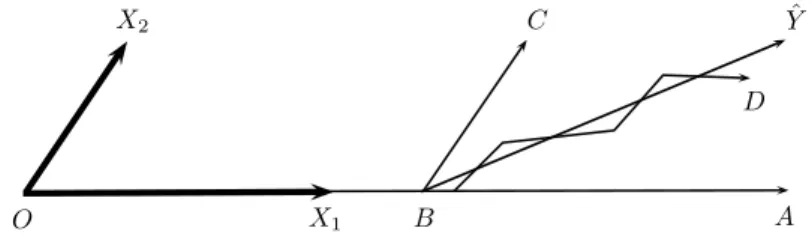
LARS can be viewed as a version of stagewise that uses mathematical for-mulas to accelerate the computations. Rather than taking many tiny steps with the first variable, the appropriate number of steps is determined algebraically, until the second variable begins to enter the model. Then, rather than taking alternating steps between those two variables until a third variable enters the model, the method jumps right to the appropriate spot. Figure 1.1 shows this process in the case of 2 predictor variables, for linear regression. In this figure,
O is the prediction based solely on an intercept. Yˆ = ˆβ1X1 + ˆβ2X2 is the ordi-nary least-squares fit, the projection of the response vectorY onto the subspace spanned byX1 andX2. Ais the forward stepwise fit after one step; the second
step proceeds to Yˆ. Stagewise takes a number of tiny steps fromO toB, then takes steps alternating between the X1 and X2 directions, eventually reaching
D; if allowed to continue it would reach Yˆ. LARS jumps from O toB in one step, whereB is the point such thatBYˆ bisects the angle ABC. At the second step it jumps toYˆ. LASSO follows a path fromO toB, then fromB toYˆ. Here LARS agrees with LASSO and stagewise (as the step size → 0for stagewise). In higher dimensions additional conditions are needed for exact agreement to hold. X1 X2 O B C A ˆ Y D
Figure 1.1: The LARS algorithm in the case of2predictors.
The first variable chosen is the one that has the smallest angle between the variable and the response variable; in Figure1.1the angleY OXˆ 1 is smaller than
ˆ
Y OX2. We proceed in that direction as long as the angle between that pre-dictor and the vector of residuals Y −ξX1 is smaller than the angle between other predictors and the residuals. Eventually the angle for another variable will equal this angle (once we reach pointB in Figure1.1 ), at which point we begin moving toward the direction of the least-squares fit based on both vari-ables. In higher dimensions we will reach the point at which a third variable has an equal angle and will join the model, etc.
It has been shown that there is a correspondence between the geometric con-cept of angle and the statistical concon-cept of correlation in a linear model. Ex-pressed another way, the (absolute value of the) correlation between the resid-uals and the first predictor is greater than the (absolute) correlation for other predictors. Asξ increases, another variable will eventually have a correlation with the residuals equaling that of the active variable, and join the model as a second active variable. In higher dimensions additional variables will eventu-ally join the model, when the correlation between all active variables and the residuals gradually drops to the levels of the additional variables.
that “The entire sequence of LARS steps with p < nvariables requiresO(p3 +
np2) computations - the cost of a least squares fit on p variables.” Second is that the basic LARS algorithm, based on the geometry of angle bisection, can be used to efficiently fit LASSO and stagewise models, with certain modifications in higher dimensions [29]. This provides a fast and relatively simple way to fit LASSO and stagewise models. Third is the availability of a simple Cp statistic
as a stopping criterion of the algorithm,
Cp = ˆσ−2 n
X
i=1
(yi−yˆi)2−n+ 2k
where k is the number of steps and σ2 is the estimated residual variance (es-timated from the saturated model, assuming that n > p, or in some other way if p ≥ n in order to deal with overfitting). This is based on Theorem
3 in [29], which indicates that after k steps of LARS the degrees of freedom
Pn
i=1cov(ˆµi, Yi)/σ
2 is approximatelyk. This provides a simple stopping rule, to stop after the number of stepskthat minimizes theCpstatistic. Note that there
are different definitions of degrees of freedom, and the one used here is appro-priate for theCp statistic, but thisk does not measure other kinds of degrees of
freedom.
1.1.2 Comparing LARS, LASSO and Stagewise
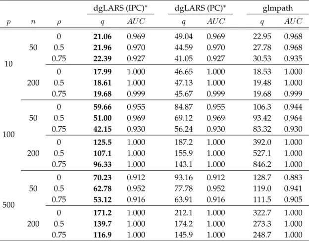
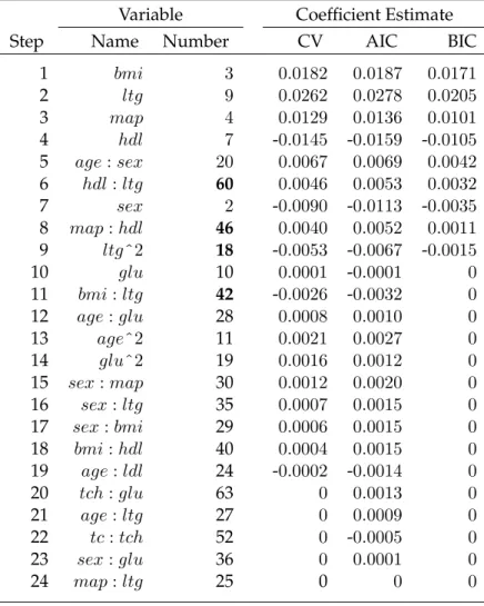
In general in higher dimensions native LARS and the least angle implemen-tation of LASSO and stagewise give results that are similar but not identical. When they differ, LARS has a speed advantage, because LARS variables are added to the model, never removed. Hence it will reach the full least-squares solution, using all variables, inpsteps. For LASSO, and to a greater extent for stagewise, variables can leave the model, and possibly re-enter later, multiple times. Hence they may take more thanpsteps to reach the full model (ifn > p). [29] test the three procedures for the diabetes data using a quadratic model, con-sisting of the10main effects,45two-way interactions, and9squares (excluding the binary variable "sex"). LARS takes64steps to reach the full model, LASSO takes 103, and stagewise takes 255. Even in other situations, when stopping short of the saturated model, LARS has a speed advantage.
an l1 penalty, a relatively simple concept; this is also known as a form of reg-ularization in the machine learning community. Stagewise is closely related to boosting, or ‘slow learning’ in machine learning [29, 43]. LARS has a simpler interpretation than the original derivation; it can be viewed as a variation of Newton’s method, which makes it easier to extend to some nonlinear models such as generalized linear models [82].
1.2
Elementary Differential Geometry
For information geometry the most important aspects of differential geome-try are those which allow us to take problems from a variety of fields: statistics, information theory, and control theory; visualize them geometrically; and from this develop novel tools with which to extend and advance these fields. In this section we present an introduction to differential geometry from this point of view, and at the end of the section we present a geometric structure of statistical models.
1.2.1 Differentiable Manifolds
A differentiable manifold is a mathematical concept denoting a generaliza-tion/abstraction of geometric objects such as smooth curves and surfaces in an
n-dimensional space. Intuitively, a manifold S is a “set with a coordinate sys-tem.” SinceS is a set, it has elements. It does not matter what these elements are (these elements are also called thepoints ofS.) S must also have a coordi-nate system. By this we mean a one-to-one mapping from S (or its subset) toRn,
which allows us to specify each point inSusing a vector ofnreal numbers (this vector is called thecoordinatesof the corresponding point). We call the natural numbernthedimensionofS, and writen = dimS. We call a coordinate system that hasSas its domain a global coordinate system.
Let S be a manifold and φ : S → Rn be a coordinate system for S. Thenφ
maps each pointpinStonreal numbers: φ(p) = [ξ1(p), . . . , ξn(p)] = [ξ1, . . . , ξn]. These are the coordinates of the pointp. Each ξi may be viewed as a function
p → ξi(p)which maps a point pto its ith coordinate; we call these n functions
ξi : S → R(i = 1, . . . , n)the coordinate functions. We shall write the coordinate systemφin ways such asφ= [ξ1, . . . , ξn] = [ξi].
Letψ = [ρi]be another coordinate system forS. Then the same pointp∈ S
has both the coordinates[ξi(p)] = [ξi] ∈ Rnwith respect to the coordinate
sys-tem φ, and the coordinates [ρi(p)] = [ρi] ∈ Rn with respect to the coordinate
system ψ. The coordinates[ρi]may be obtained from[ξi]in the following way. First apply the inverse mapping φ−1 to[ξi]; this gives us a pointpin S. Then
applyψ to this point; this result is[ρi]. In other words, we apply the
transfor-mation onRngiven by
ψ◦φ−1 : [ξ1, . . . , ξn]7→[ρ1, . . . , ρn] (1.1) This is called thecoordinate transformationfromφ= [ξi]toψ = [ρi].
Let S be a set. If there exists a set of coordinate systems A for S which satisfies the conditions (i) and (ii) below, we call S (more properly, (S,A)) an
n-dimensionalC∞differentiable manifold, or more simply, amanifold.
(i) Each elementφofAis a one-to-one mapping fromSto some open subset of Rn.
(ii) For allφ∈ A, given any one-to-one mappingψfromStoRn, the following
holds:
ψ ∈ A ⇐⇒ψ◦φ−1 is a C∞diffeomorphism.
Here, by a C∞ diffeomorphism we mean that ψ◦φ−1 and its inverseφ◦ψ−1 are both C∞(infinitely many times differentiable). From these conditions, and given the coordinate transformation described in Equation (1.1), it follows that we may take the partial derivative of the functionρi =ρi(ξ1, . . . , ξn)with respect
to its variable arguments as many times as needed, and that the same holds for
ξi =ξi(ρ1, . . . , ρn).
LetS be a manifold andφbe a coordinate system for S. Let U be a subset ofS. If the imageφ(U)is an open subset of Rn, then we say thatU is an open
subset ofS. From condition (ii) above, we see that this property is invariant over the choice of coordinate systemφ. This allows us to considerS as a topological space.
1.2.2 Tangent Vectors and Tangent Spaces
Thetangent spaceTp at a pointp ∈ S of a manifoldS is intuitively the vector
system for S, and let ei denote the tangent vector which goes through point p
and is parallel to theithcoordinate curve (coordinate axis). By theithcoordinate curve we mean the curve which is obtained by fixing the values of all ξj for
j ̸=iand varying only the value ofξj. Then-dimensional space spanned by the n tangent vectorse1, . . . ,enis the tangent spaceTp at pointp. Letp′ be a point
"very close" top, and let[ξi]and[ξi+dξi](where dξi is an infinitesimal) be the
coordinates ofpandp′, respectively. Then the segment joining these two points may be described by−→p p′ =dξie
i, an infinitesimal vector inTp.
1.2.3 Submanifolds and Riemannian Metrics
Let S and Mbe manifolds, whereMis a subset of S. Let [ξ1, . . . , ξn] = [ξi]
and[u1, . . . , um] = [ua]be coordinate systems forS and M, respectively, where
n = dimS and m = dimM. Below, we shall use the indices i, j, k, . . . over {1, . . . , n}forS anda, b, c, . . .over{1, . . . , m}forM.
We callMasubmanifoldofSif the following conditions (i), (ii), and (iii) hold.
(i) The restrictionξi|
Mof eachξi (:S → R) toM, is a C∞function onM. (ii) Let Bi a def = ∂u∂ξia p (more precisely, ∂ξi|M ∂ua p) and Ba def = [B1 a, . . . ,Ban] ∈ Rn.
Then for each pointpinM,{B1, . . . ,Bm}are linearly independent (hence
m≤n).
(iii) For any open subsetWofM, there existsU, an open subset ofS, such that
W =M ∩ U.
These conditions are independent of the choice of coordinate systems [ξi]
and [ua]. Indeed, conditions (i) and (ii) mean that the embedding ι : M → S
denned byι(p) = p, ∀p ∈ M, is a C∞ mapping and that its differential(dι)p is
nondegenerate at each pointp.
Let S be a manifold. For each point p in S, let us assume that an inner product ⟨ , ⟩p has been denned on the tangent space TP(S). In other words,
for any tangent vectorsD,D′ ∈TP(S)we have⟨D, D′⟩p ∈ R, and the following
hold.
• Linearity
• Symmetry
⟨D, D′⟩p =⟨D′, D⟩p, (1.3)
• Positive-definiteness
IfD̸= 0then⟨D, D⟩p >0 (1.4)
Note that⟨, ⟩p ∈ [Tp(S)]02 since from Equations (1.2) and (1.3) we see that⟨, ⟩p
is a bilinear form. Hence the mapping from pointspinS to their inner product onTP(S), sayg : p7→ ⟨, ⟩p, is a tensor field of covariant degree2. We call this
a (C∞)Riemannian metriconS. Such a metric,g, is not naturally determined by the structure ofS as a manifold; it is possible to consider an infinite number of Riemannian metrics onS. Given a Riemannian metricg on S, we callS (more precisely(S, g)) aRiemannian manifold.
Also, the length∥D∥of the tangent vectorDis given by ∥D∥2 =⟨D, D⟩p =gij(p)DiDj.
Another important property that we will make use of, is the following: two vectors areorthogonalif⟨D, D′⟩= 0. The Schwarz inequality
⟨D, D′⟩ ≤ ∥D∥∥D′∥
allows the angle0≤ϑ≤πbetween vectors to be defined by
cosϑ= ⟨D, D ′⟩
∥D∥∥D′∥.
1.2.4 The Geometric Structure of Statistical Models
Consider a familySof probability distributions onX. Suppose each element ofS, a probability distribution, may be parameterized usingnreal-valued vari-ables[ξ1, . . . , ξn]so that
S =
where p is a probability density function on X, Ξ is a subset of Rn and the
mappingξ 7→pξis injective. We call suchS ann-dimensionalstatistical model, a
parametric model, or simply amodelonX. We will often abbreviate Equation (1.5) asS = {pξ}, and also use expression such as pξ(x) = p(x;ξ)andS ={p(x;ξ)}.
When we say "a statistical model S = {pξ}," there shall be cases in which we
refer simply to the set S, and other cases in which we refer in addition to the parameterizationξ 7→pξ.
Let S = {pξ | ξ ∈ Ξ} be ann-dimensional statistical model. Given a point
ξ(∈,Ξ), theFisher information matrixofS atξis then×nmatrixG(ξ) = [gij(ξ)]
where the(i, j)th elementgij(ξ)is defined by the equation below; in particular,
whenn= 1, we call this theFisher information.
gij(ξ) def = Eξ[∂iℓξ∂jℓξ] = Z ∂iℓ(x;ξ)∂jℓ(x;ξ)p(x;ξ)dx, (1.6) where∂i def = ∂ξ∂i, ℓξ(x) = ℓ(x;ξ) = logp(x;ξ). (1.7)
We note that it is possible to writegij as
gij(ξ) =−Eξ[∂i∂jℓξ].
Let S = {pξ} be an n-dimensional model, and consider the function Γ
(α)
ij,k
which maps each pointξto the following value: Γ(ij,kα) ξ def = Eξ ∂i∂jℓξ+ 1−α 2 ∂iℓξ∂jℓξ (∂kℓξ) , (1.8)
whereαis some arbitrary real number. We have an affine connection∇(α)onS defined by
⟨∇(∂αi)∂j, ∂k⟩= Γ
(α)
ij,k, (1.9)
α-connection is clearly a symmetric connection. We also have ∇(α) = (1−α)∇(0)+α∇(1) = 1 +α 2 ∇ (1)+1−α 2 ∇ (−1). (1.10) In addition, for a submanifold M of S, the α-connection on Mis simply the projection with respect togof theα-connection onS.
Let us introduce now the notion of exponential family, which will be shown to have close relation to∇(1). In general, if ann-dimensional modelS ={p
θ|θ∈
Θ}can be expressed in terms of functions {C, F1, . . . , Fn}on X and a function
ψ onΘas p(x;θ) = exp " C(x) + n X i=1 θiFi(x)−ψ(θ) # , (1.11)
then we say that S is an exponential family, and that the [θi] are its natural or
its canonical parameters. From the normalization condition R
p(x;θ)dx = 1 we obtain ψ(θ) = log Z exp " C(x) + n X i=1 θiFi(x) # dx. (1.12)
It is easy to see that the parametrizationθ 7→ pθ is one-to-one if and only if the
n + 1 functions {F1, . . . , Fn,1} are linearly independent, where 1 denotes the
constant function which identically takes the value1. For more details see [6].
1.3
Exponential Dispersion GLMs
This section is devoted to a brief review of the theory of dispersion models (DM) based primarily on Jørgensen’s book [51], The theory of dispersion models. The dispersion models provide a rich class of one-dimensional parametric dis-tributions for various data types, including those commonly considered in the GLM analysis. In effect, error distributions in the GLMs form a special subclass of the dispersion models, which are theexponential dispersion (ED)models. This means that the GLMs considered in [51] encompass a wider scope of GLMs than those outlined in McCullagh and Nelder’s book [60], however, we will focus on
only the ED models. Two special examples are the von Mises distribution for directional (circular or angular) data and thesimplexdistribution for composi-tional (or proporcomposi-tional) data, both of which are the dispersion models but not the exponential dispersion models. First, let’s introduce the DM.
1.3.1 Dispersion Models
Mimicking the density of the normal distribution N(µ, σ2), [51] defines a dispersion models by extending the Euclidean distance(y−µ)2, that measures the discrepancy between the observed y and the expectedµ, to a general dis-crepancy function d(y;µ). It is found that many commonly used parametric distributions, such as Binomial, Poisson and Gamma, are included as special cases of this extension. Moreover, each of such distributions will be determined uniquely by the discrepancy functiond, and the resulting distribution is fully parameterized by two parametersµandσ2.
A (reproductive)dispersion modelDM(µ, σ2) with location parameterµand dis-persion parameterσ2 is a family of distributions whose probability density func-tions take the following form:
p(y;µ, σ2) =a(y;σ2) exp
−21σ2 d(y;µ)
, y∈ C, (1.13)
where µ ∈ Ω, σ2 > 0, and a ≥ 0 is a suitable normalizing term that is inde-pendent of the µ. Usually, Ω ⊆ C ⊆ R. The fact that the normalizing term a
does not involveµwill allow to estimateµ(orβin the GLM setting) separately from estimatingσ2, which gives rise to great ease in the parameter estimation. This a nice property, known as the likelihood orthogonality, holds in the normal distribution, and is a feature in dispersion models.
A bivariate functiond(·;·)is called theunit deviancedefined on(y, µ)∈ C ×Ω
if it satisfies the following two properties: i) It is zero when the observedyand the expectedµare equal, namelyd(y;y) = 0, ∀y ∈ Ω; ii) It is positive when the observedyand the expectedµare different, namelyd(y;µ)>0, ∀y̸=µ.
Furthermore, a unit deviance is calledregularif functiond(y;µ)is twice con-tinuously differentiable with respect to(y, µ)onΩ×Ωand satisfies
∂2d ∂µ2(y;y) = ∂2d ∂µ2(y;µ) µ=y >0, ∀y∈Ω.
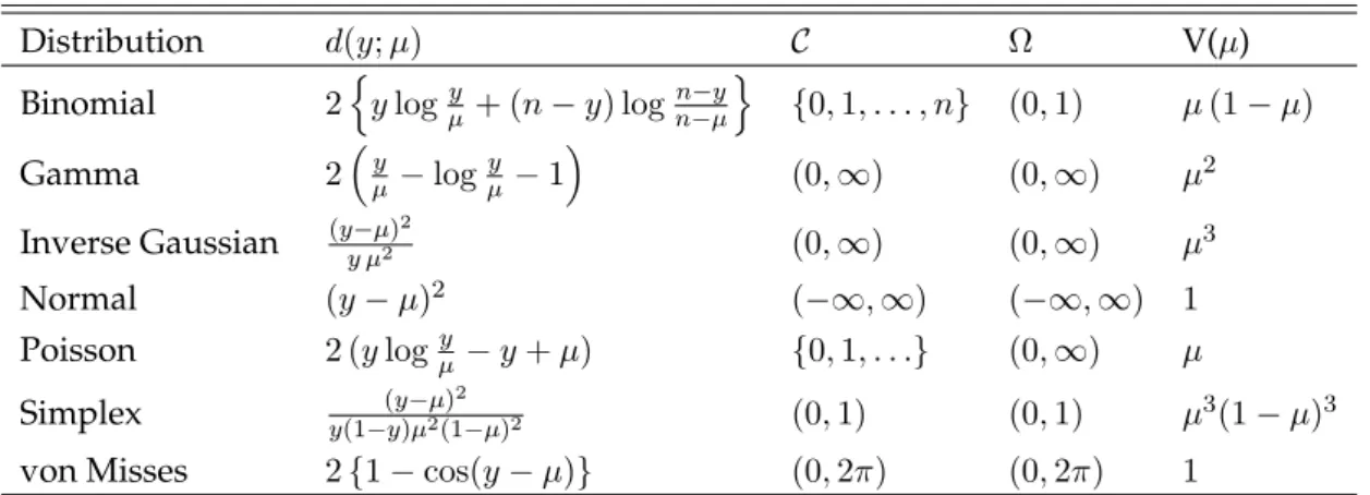
Table 1.1: Unit deviance and variance functions of some dispersion models.
Distribution d(y;µ) C Ω V(µ)
Binomial 2nylogµy + (n−y) lognn−−µyo {0,1, . . . , n} (0,1) µ(1−µ)
Gamma 2µy −logµy −1 (0,∞) (0,∞) µ2 Inverse Gaussian (yy µ−µ2)2 (0,∞) (0,∞) µ3 Normal (y−µ)2 (−∞,∞) (−∞,∞) 1 Poisson 2 (ylogyµ−y+µ) {0,1, . . .} (0,∞) µ Simplex y(1−(yy)−µ2µ(1)2−µ)2 (0,1) (0,1) µ 3(1 −µ)3
von Misses 2{1−cos(y−µ)} (0,2π) (0,2π) 1
For a regular unit deviance, the variance function is defined as follows. The unit variance functionV : Ω→(0,∞)is
V(µ) = 2
∂2d
∂µ2(y;µ)|y=µ
, µ∈Ω. (1.14)
Some popular dispersion models are given in Table1.1.
1.3.2 GLMs based on the Exponential Dispersion Models
The class of dispersion models contains two important subclasses, namely theexponential dispersion(ED)modelsand the proper dispersion(PD)models. The PD models are mostly of theoretical interest, so they are not discussed in this thesis. Readers may refer to [51] for relevant details.
This section focuses on the ED models, which have already been introduced at the beginning of Section1.3as a family of GLMs’ error distributions. The fam-ily of ED models includes continuous distributions such as Normal, Gamma, and Inverse Gaussian, and discrete distributions such as Poisson, Binomial, Negative Binomial, among others.
According to [60], the random component of a GLM is specified by an expo-nential dispersion family density of the following form:
p(y;θ, ϕ) = exp yθ−b(θ) a(ϕ) +c(y, ϕ) , y∈ C, (1.15)
gen-erating function andC is the support of the density. It is known that the first derivative of the cumulant functionb(·) gives the expectation of the distribu-tion, namely µ = E(Y) = b′(θ), where b′(θ) = ∂b∂θ(θ), and the variance of the distribution is Var(Y) = a(ϕ)V(µ). This mean-variance relationship is one of the key properties for the ED models, which will play an important role in the development of quasi-likelihood inference.
The systematic component of a GLM is then assumed to take the form:
g(µ) =x⊤β =β0+β1x1+. . .+βpxp (1.16)
wheregis the link function,x= (1, x1, . . . , xp)⊤is a(p+1)-dimensional vector of
covariates, andβ= (β0, β1, . . . , βp)⊤is a(p+1)-dimensional vector of regression
coefficients. Thecanonicallink functiong(·)is such thatg(µ) = θ, the canonical parameter. The primary statistical tasks include estimation and inference forβ. To establish the connection of the ED model representation (1.15) to the DM, it is sufficient to show that expression (1.15) is a special form of (1.13). An advantage with the DM type of parametrization for the ED models is that both meanµand dispersion parametersσ2 are explicitly present in the density, whereas expression (1.15) hides the mean µ in the first order derivative b′(θ). In addition, having a density form similar to the normal enables us to easily borrow the classical normal regression theory to the development of regression analysis for non-normal data.
To reparametrize this density (1.15) by the meanµand dispersionσ2, denote
a(ϕ) = σ2 and define themean value mapping: τ :int(Θ)→Ω,
τ(θ) =b′(θ)≡µ,
whereint(Θ)is the interior of the parameter spaceΘ. The mean mapping func-tion τ(θ) is strictly increasing and its inverse exists, denoted by θ = τ−1(µ),
µ∈Ω.
As a result, the density of an ED model in (1.15), denoted by ED(µ, σ2), can be expressed as of the DM form in (1.13) with the unit deviance functiondgiven by d(y;µ) = 2 sup θ∈Θ{ θy−b(θ)} −y τ−1(µ) +b(τ−1(µ)) , (1.17)
and the normalizing term given by a(y;σ2) = c(y;σ−2) exp σ−2sup θ∈Θ{ θy−b(θ)} . (1.18)
Clearly, this d function (1.17) satisfies (i) d(y;µ) ≥ 0 for all y ∈ C and µ ∈ Ω, and (ii) d(y;µ) attains the minimum at µ = y because the supremum term is independent ofµ. Thus, (1.17) gives a proper unit deviance function. Moreover, since it is continuously twice differentiable, it is also regular.
An important variant of the reproductive ED model representation is the so-calledadditive exponential dispersion model, denoted by ED∗(θ, λ), whose density takes the form
p∗(z;θ, λ) =c∗(z;λ) exp{θ z−λ b(θ)}, z ∈ C, (1.19) The Gamma and Inverse Gaussian distributions are members of the ED∗ and ED families, respectively. Essentially the ED and ED∗ representations are equivalent under theduality transformationthat converts one form to the other. Suppose Z ∼ ED∗(θ, λ) and Y ∼ ED(µ, σ2). Then, the duality transformation performs
Z ∼ED∗(θ, λ)⇒Y =Z/λ∼ED(µ, σ2), with µ=τ(θ), and σ2 = 1/λ;
Y ∼ED(µ, σ2)⇒Z =Y /σ2 ∼ED∗(θ, λ), with θ =τ−1(µ), and λ= 1/σ2.
Consequently, the mean and variance of ED∗(θ, λ)are, respectively,
µ∗ =E(Z) =λ τ(θ), and Var(Z) =λ V(µ∗/λ).
An important property for these models is closure under the convolution operation.
Convolution for theED∗ models. Assume Z1, . . . , Zn are independent and
Zi ∼ED
∗
(θ, λi), i= 1, . . . , n, then the sum follows still an ED
∗ model: Z+ = n X i=1 Zi ∼ED ∗ (θ, n X i=1 λi).
Yi ∼ ED(µ,σ
2
wi), wherewis are certain positive weights. Letw+ =w1+. . .+wn, then 1 w+ n X i=1 wiYi ∼ED(µ, σ2 w+ ).
We note that although the class of the ED models is closed under the convo-lution operation, it is in general not closed under scale transformation. That is,
cY may not follow an ED model even if Y ∼ ED(µ, σ2), for a constantc. How-ever, a subclass of the ED models, termed as theTweedie class, is closed under this type of scale transformation. Tweedie class is an important subclass of the ED models. Tweedie models are characterized by the unit variance functions in the form of the power function:
Vp(µ) =µp, µ∈Ωp, (1.20)
wherep∈Ris a shape parameter. It is shown that the ED model with the power unit variance function (1.20) always exists except0 < p < 1. Special cases in-clude the Normal (p= 0), Poisson (p= 1), Gamma (p= 2) and Inverse Gaussian (p = 3). Another interesting class of Tweedie GLMs is for values of pbetween
1 and 2. In this interval, closed form distribution functions do not exist, but Tweedies in this interval are compound Poisson distributions. (A compound Poisson random variableY is the sum ofN independent Gamma random vari-ables where N follows a Poisson distribution andN and the Gamma random variates are independent.) A Tweedie model is denoted byY ∼T wp(µ, σ2)with
meanµand variance
Var(Y) =σ2µp.
1.3.3 MLE in the Exponential Dispersion GLMs
This section is devoted to maximum likelihood estimation in the GLMs based on the ED models. Consider (yi,xi), i = 1, . . . n, as a dataset where the yis
are i.i.d. realizations of Yis according to ED(µi, σ2) and g(µi) = x⊤i β . Let
y= (y1, . . . , yn)⊤andµ= (µ1, . . . , µn)⊤. The likelihood for the parameter vector
θ= (β, σ2)is given by L(θ;y) = n Y i=1 a(yi;σ2) exp − 1 2σ2 d(yi;µi) , β ∈ Rp+1 , σ2 >0,
and the log-likelihood is then ℓ(θ;y) = n X i=1 loga(yi;σ2)− 1 2σ2 D(y;µ), (1.21) where D(y;µ) = Pn
i=1d(yi;µi) is the sum of deviances depending on β only andµi =µi(β)is a nonlinear function inβ.
Thescore functionfor the regression coefficientβis
s(y;β) = ∂ℓ(θ) ∂β =− 1 2σ2 n X i=1 ∂d(yi;µi) ∂µi ∂µi ∂β = 1 σ2 n X i=1 xi (yi−µi) g′(µ i)V(µi) (1.22) because in this case
∂d(yi;µi) ∂µi =−2(yi −µi) V(µi) and ∂µi ∂β = ∂µi ∂ηi ∂ηi ∂β ={g ′ (µi)}−1xi
where ηi = x⊤i βis theith linear predictor, andg′(µ)is the first order derivative
of the link functiong w.r.t.µ.
Moreover, the score equation leading to the maximum likelihood estimate of
βis n X i=1 xi (yi−µi) g′(µ i)V(µi) =0, (1.23)
such that it can be re-expressed in matrix form as
X⊤W−1(y−µ) =0,
where X is a n × (p + 1) matrix with the ith row being the x⊤i , and W =
diag(w1, . . . , wn)withwi =g′(µi)V(µi).
Note that this equation does not involve the dispersion parameterσ2. Under some mild regularity conditions, the resulting ML estimator βˆn, which is the
solution to the score equation (1.23), is consistent
ˆ βn
p
and asymptotically normal with mean 0and covariance matrix I−1(θ). Here,
I(θ)is theFisher information matrix, which is an(p+ 1)×(p+ 1)matrix, given by I(θ) =−E ∂s(y;β) ∂β = 1 σ2 n X i=1 xiu−i1x ⊤ i =X⊤U−1X/σ2, (1.24)
where U is a diagonal matrix with the ith diagonal element ui given by ui = {g′(µi)}2V(µi). It consists of the elementsIij(θ) = E[∂ℓ∂β(θ;y)i ∂ℓ∂β(θ;y)j ]. The Fisher
information, which is the expected value of the observed information, gives information about the efficiency of the maximum likelihood. It determines the conditional correlation between βi and βj and we say that two parameters βi
andβj are orthogonal if the element of theithrow andjth column of the Fisher
information matrix is zero.
It is interesting to note that the choice of the canonical link function g =
τ−1(·)simplifies both score function and Fisher information. Under the canoni-cal link function, the score equation of an ED GLM is
n
X
i=1
xi(yi−µi) =0, or X⊤(y−µ) = 0,
and the Fisher information takes the form
I(θ) =X⊤U−1X/σ2
whereUis a diagonal matrix whoseithdiagonal element given byui = 1/V(µi).
Because, in this case, wi = 1 and g′(µi) = 1/V(µi), the matrix W becomes the
identity matrix and the matrixUis determined by the reciprocals of the variance functions.
When the dispersion parameter σ2 is present in the model, the ML estima-tion for the dispersion parameterσ2can be derived similarly, if the normalizing terma(y;σ2)is simple enough to allow such a derivation, such as the case of the normal distribution. However, in many cases, the terma(·)has no closed form
expression and its derivative w.r.t. σ2 may appear too complicated to be nu-merically solvable. In this case, three methods have been suggested to acquire the estimation for σ2. The first method, which is referred to as the Jørgensen estimator of the dispersion parameter, is
ˆ σ2d= 1 nD(y; ˆµ) = 1 n n X i=1 d(yi; ˆµi), (1.25)
where the indexdstands fordeviance. This estimator, in fact, is an average of the estimated unit deviances. However, this estimator is not, in general, unbiased even if the adjustment on the degrees of freedom,n−(p+ 1), is made to replace
n. Moreover, this formula is recommended when the dispersion parameterσ2
is small, say less than5. For more details about this estimator see [51] and [60]. Each ED model holds the so-called mean-variance relation, i.e., Var(Y) =
σ2V(µ), which may be used to obtain a consistent estimator of the dispersion parameterσ2 given as follows:
ˆ σP2∗ = 1 n−p−1 n X i=1 (yi−µˆi)2 V(ˆµi) . (1.26)
This second method, which utilizes a moment property, is referred to as the Pearsonestimator of the dispersion parameterσ2. The third method is the max-imum likelihood (ML) method. The ML estimator of the dispersion parameter
σ2is the solution of∂ℓ(βˆ, σ2;y)/∂σ2 = 0. More information about this estimator
ˆ
σmle2 can be found in [51] and [60].
1.3.4 A Differential Geometrical Description of the GLM
In this section we introduce the GLM from a differential geometric point of view. In our treatment, we rely heavily on [5], [53] and [6]. A differential geo-metric approach was also used in [98] to study non-linear models based on the exponential family. Essential aspects of differential and information geometry have been included in this section.
vec-torYcan be written as pY(y;θ, ϕ) = n Y i=1 pYi(yi;θi, ϕ), (1.27)
whereY = (Y1, Y2, . . . , Yn)⊤is a random vector with independent components,
Yi is assumed to be a random variable with probability density function
be-longing to the family (1.15), and the canonical parameterθ varies in the subset ⊗n
i=1Θi = Θ⊆ Rn. As mentioned in Section1.3.2, E(Y) =µ= (τ(θ1), . . . , τ(θn))⊤,
whereτ(θi) = b′(θi)≡µiis called mean value mapping, and Var(Y) =a(ϕ)V(µ),
whereV(µ) =diag(V(µ1), . . . , V(µn)is ann×ndiagonal matrix whereV(µi) =
b′′(θi)is called the variance function. From Section1.3.2we haveτ :int(Θ)→Ω
so thatτ(·)is a one-to-one function, thereforepY(y;θ, ϕ)may be parameterized bypY(y;µ, ϕ), as described in Section1.3.1 and 1.3.2. To simplify our notation we will assume thatϕ = 1[53]. Assuming thatΘis open, the set
S ={pY(y;µ) :µ∈Ω} (1.28)
is a minimal and regular exponential family of order n and can be treated as a differential manifold where the parameter vector µ plays the role of a co-ordinate system [5]. The notion of differential manifold is necessary for extend-ing the methods of differential calculus to a space that is more general thanRn.
For a rigorous definition of a differential manifold the reader is referred to [90] and [21]. It is worth noting that the results coming from differential geometry are not related to the chosen co-ordinate system, i.e., the parameterization that is used to specify the probability density function (1.15). This means that we could work with the differential manifold S using the parameter vector θ as co-ordinate system. In this thesis we prefer to use definition (1.28) only because we believe that this makes the generalization of the LARS algorithm clearer.
Following [60], a Generalized Linear Model (GLM) is defined by means of a known functiong(·), called link function, relating the expected value of eachYi
to the vector of covariatesxi = (1, xi1, . . . , xip)⊤by the identity
g{E(Yi)}=ηi =x⊤i β
of regression coefficients with the intercept andpparameters. In order to sim-plify our notation we letµ(β) = {µ1(β), . . . , µn(β)}⊤ whereµi(β) = g−1(x⊤i β).
Therefore, the probability density function can be written as pY(y;µ(β), ϕ) =
Qn
i=1pYi(yi;µi(β), ϕ).
In order to study the geometrical structure of a GLM, we shall assume that
β → {g−1(x⊤
1β), . . . , g
−1(x⊤
nβ)}
⊤ = µ(β)
is an embedding, this means that the set
M={pY(y;µ(β))∈ S :β ∈ Rp+1
}
is ap+ 1-dimensional submanifold ofS, which inherits the dualistic structure from its ambient space, then, as a simple consequence of theorem 3.5 in [6], M is a dually flat space only when we work with the canonical link function. To obtain a natural generalization of the equiangularity condition that was pro-posed by [29], it is necessary to introduce two fundamental notions on which Riemannian geometry is based: the notions of a tangent space and a Rieman-nian metric. To complete the differential geometric setting for the GLM, we shall assume that the usual regularity conditions hold [5, page 16]. Throughout this paper we use the convention that the indices i, j and k correspond to the quantities that are related toµ ∈ Ωwhereas the indices l, m and qcorrespond to the quantities that are related to the coefficients β ∈ Rp+1 of our regression model.
Consider a double-differentiable curve, sayµ : Γ → Ω, whereΓ is the real interval (−δ, δ) with δ > 0. The tangent vector to the one-parametric family
pY(y;µ(γ))atµ=µ(0)is defined as v(Y) = dℓ(µ(γ);Y) dγ γ=0 = n X i=1 dµi(0)∂iℓ(µ;Y), (1.29)
where dµi(0) = dµi(γ)/dγ|γ=0 and ∂iℓ(µ;Y) = ∂log{pY(Y;µ(γ))}/∂µi|γ=0. Roughly speaking, the tangent space of S at the point pY(y;µ) denoted by
Tp(µ)S, is the set of all possible tangent vectors at µ = µ(0). Formally, Tp(µ)S is the vector space that is spanned by thenscore functions∂iℓ(µ;Y):
Tp(µ)S =span{∂1ℓ(µ;Y), ∂2ℓ(µ;Y), . . . , ∂nℓ(µ;Y)}. (1.30)
integrable random variables, in which elements v(Y) satisfy the property Eµ{v(Y)} = 0, where the expected value is computed with respect to pY(y;µ). As an application of the chain rule, it is easy to see that the definition of a tan-gent space does not depend on the chosen parameterization; in other words the tangent space can be defined as the vector space that is spanned by thenscore functions ∂i∗ℓ(θ;Y) = ∂log{pY(Y;θ(γ))}/∂θi|γ=0 where θ(γ) = θ(µ(γ)). Using the terminology that was introduced in [97], ∂iℓ(µ;Y) are the natural bases of
the tangent space when we chooseµas co-ordinate system, whereas ∂i∗ℓ(θ;Y)
are the natural bases whenθis used as the co-ordinate system.
Similarly, consider a double-differentiable curve β : Γ′ → Rp+1, with Γ′ = (−δ′, δ′)andδ′ >0. The tangent vector to the one-parametric familypY(y;µ(β(γ)))
at the pointβ=β(0)is defined as
w(Y) =
p
X
m=1
dβm(0)∂mℓ(β;Y),
wheredβm(0) =dβm(γ)/dγ|γ=0 and∂mℓ(β;Y) = ∂log{pY(Y;µ(β(γ)))}/∂βm|γ=0. Then, the tangent space ofMat the pointpY(y;µ(β))is
Tp(µ(β))M=span{∂1ℓ(β;Y), ∂2ℓ(β;Y), . . . , ∂nℓ(β;Y)}. (1.31)
The definition of the inner product on each tangent space allows us to generalize the notion of angle between two curves, say µ1(γ) and µ2(γ), intersecting at
µ1(0) =µ2(0) =µ, with tangent vectors belonging toTp(µ)S, denoted by
v1(Y) = n X i=1 dµ1,i(0)∂iℓ(µ;Y) and v2(Y) = n X i=1 dµ2,i(0)∂iℓ(µ;Y)
respectively. When working with a parametric family of distributions, the inner product can be defined in a natural way [78], i.e.
whereI(µ)is the Fisher information matrix for the mean parameter at pointµ. In other words, the Fisher information defines a Riemannian metric by associ-ating with each point ofS an inner product on the tangent space. This Rieman-nian metric is also called the information metric[17]. SinceTp{µ(β)}Mis a linear
subspace ofTp{µ(β)}S, the Fisher information also defines an inner product on
Tp{µ(β)}M. Therefore, we can define the inner product between a tangent vector
w(Y)ofTp{µ(β)}Mand a tangent vectorv(Y)ofTp{µ(β)}S, namely
⟨w(Y), v(Y)⟩p{µ(β)} =Eµ(β){v1(Y)v2(Y)}=dβ(0)⊤
∂µ(β)
∂β ⊤
I{µ(β)}dµ(0),
where∂µ(β)/∂βis the Jacobian matrix of the vector functionµ(β).
Each Riemannian metric defines the notion of a geodesic, i.e. the generaliza-tion of a straight line in a differential geometric framework. Roughly speaking, a geodesic can be defined as the shortest path between two given points on a differential manifold. A geodesic is defined as the solution of a system of differential equations, the Euler–Lagrange equations, obtained from defining a connection on a differentiable manifold. In statistical theory a one-parametric family of connections plays a fundamental role, the so-called α-connections, denoted by∇α, that generalize the classical notion of a Levi–Civita connection,
which is the special case that α = 0. In the theory of information geometry, ∇0 is also called the information connection since it is derived from the Fisher information. What is also important for what follows in this thesis is that S is a dually flat space, namely, it is flat with respect to the 1- and −1-connection. For more details of this dual geometry, the reader is referred to [6]. As shown in [97], associated with the−1-connection and each pointpY(y;µ)∈ S there is a diffeomorphism between a neighbourhood of the origin inTp(µ)S and a neigh-bourhood ofpY(y;µ), called the−1-exponential map. The dual nature that exists between∇−1and∇1defines the dual of the−1-exponential map, namely the so-called1-exponential map. SinceS is a dually flat space, the inverses of the two exponential maps are well defined on all S and for eachpY(y;µ). To complete the geometrical framework that is needed to generalize the LARS algorithm in next chapter, we consider the inverse of the−1-exponential map, which relates the observed response variable y to the tangent spaces. [97] defined what we
call thetangent residual vector r(µ(β),y;Y) = n X i=1 {yi−µi(β)}∂iℓ(µ(β);Y) (1.32)
where∂iℓ(µ(β);Y) =∂ℓ(µ;Y)/∂µi|µ=µ(β). It is important to note that we define the tangent residual vector (1.32) with respect to both the fixed observations
y and the random variableY, in such a way that it is a random variable with zero expected value and finite variance, and thereforer(µ(β),y;Y)∈Tp{µ(β)}S.
[97] showed that it is possible to give a differential geometric interpretation of the maximum likelihood estimator by using the tangent residual vector and the tangent space Tp{µ( ˆβ)}M, namely βˆ is the maximum likelihood estimate of β
when the tangent residual vector is orthogonal to the tangent spaceTp{µ( ˆβ)}M. It is worth noting that this statement is well defined even ifyis not an element of the mean value parameter spaceΩ. In other words, the differential geomet-ric description of the maximum likelihood estimator can be used even if the Kullback–Leibler divergence is not defined [97].
1.4
Survival Models
Survival analysis is a commonly-used method for the analysis of failure times such as death, mechanical failure, or credit default. Within this context, a failure is also referred to as an ‘event’. Survival models can be used for the analysis of data which have three main characteristics: (1)the dependent vari-able or response is the waitingtimeuntil the occurrence of a well-defined event,
(2) observations may be censored, in the sense that for some units the event of interest has not occurred at the time the data are analyzed, and (3) there are predictors orexplanatoryvariables whose effect on the waiting time we wish to assess or control.
LetT be a non-negative random variable representing the waiting time until the occurrence of an event. For simplicity we will adopt the terminology of sur-vival analysis, referring to the event of interest asdeathand to the waiting time assurvivaltime, but the techniques to be studied have much wider applicabil-ity. They can be used, for example, to study age at marriage, the duration of marriage, the intervals between successive births, the duration of stay in a city or in a job, besides the length of life.
1.4.1 The Survival and Hazard Function
We will assume for now thatT is a continuous random variable with proba-bility density function (p.d.f.) f(t)and cumulative distribution function (c.d.f.)
F(t) = Pr{T < t}, giving the probability that the event has occurred by duration
t.
It will often be convenient to work with the complement of the c.d.f, the survivalfunction
S(t) = Pr{T ≥t}= 1−F(t) =
Z ∞
t
f(x)dx, (1.33)
which gives the probability of being alive just before durationt, or more gen-erally, the probability that the event of interest has not occurred by duration
t.
An alternative characterization of the distribution of T is given by thehazard function, or instantaneous rate of occurrence of the event, defined as
λ(t) = lim
dt→0
Pr{t ≤T < t+dt|T ≥t}
dt . (1.34)
The numerator of this expression is the conditional probability that the event will occur in the interval[t, t+dt)given that it has not occurred before, and the denominator is the width of the interval. Dividing one by the other we obtain a rate of event occurrence per unit of time. Taking the limit as the width of the interval goes down to zero, we obtain an instantaneous rate of occurrence. The conditional probability in the numerator may be written as the ratio of the joint probability that T is in the interval [t, t+dt) and T ≥ t (which is, of course, the same as the probability that t is in the interval), to the probability of the condition T ≥ t. The former may be written as f(t)dt for smalldt, while the latter is S(t) by definition. Dividing by dt and passing to the limit gives the useful result
λ(t) = f(t)
S(t), (1.35)
which some authors give as a definition of the hazard function. In words, the rate of occurrence of the event attequals the density of events att, divided by the probability of surviving to that time without experiencing the event.
Note from Equation (1.33) that−f(t)is the derivative ofS(t). This suggests rewriting Equation (1.35) as
λ(t) =−d
dtlogS(t).
If we now integrate from0totand introduce the boundary conditionS(0) = 1
(since the event is assumed not to have occurred at the beginning of the study), we can solve the above expression to obtain a formula for the probability of surviving to durationtas a function of the hazard at all durations up tot:
S(t) = exp{−
Z t
0
λ(x)dx}= exp{−Λ(t)}, (1.36) whereΛ(t)is called thecumulative hazard(or cumulative risk).
These results show that the survival and hazard functions provide alterna-tive but equivalent characterizations of the distribution ofT. Given the survival function, we can always differentiate to obtain the density and then calculate the hazard using Equation (1.35). Given the hazard, we can always integrate to obtain the cumulative hazard and then exponentiate to obtain the survival function using Equation (1.36).
1.4.2 Censoring Mechanisms
The second distinguishing feature of survival analysis is censoring: the fact that for some units the event of interest has occurred and therefore we know the exact waiting time, whereas for others there is no precise knowledge about the survival time except that it falls in some interval.
There are several mechanisms that can lead to censored data. Under cen-soring ofType I, a sample of nunits is followed for a fixed timet. The number of units experiencing the event, or the number of ‘deaths’, is random, but the total duration of the study is fixed. The fact that the duration is fixed may be an important practical advantage in designing a follow-up study.
In a simple generalization of this scheme, called fixed censoring, each unit has a potential maximum observation timeti fori = 1, . . . , nwhich may differ
from one case to the next but is nevertheless fixed in advance. The probability that unitiwill be alive at the end of her observation time isS(ti), and the total
Under censoring ofType II, a sample of n units is followed as long as nec-essary until d units have experienced the event. In this design the number of deaths d, which determines the precision of the study, is fixed in advance and can be used as a design parameter. Unfortunately, the total duration of the study is then random and cannot be known with certainty in advance.
In a more general scheme calledrandom censoring, each unit has associated with it a potential censoring time Ci and a potential lifetimeZi , which are
as-sumed to the independent random variables. We observeTi = min{Ci, Zi}, the
minimum of the censoring and life times, and an indicator variableδi =I(Zi ≤
Ci), often calledstatus, that tells us whether observation terminated by death or
by censoring.
All these schemes have in common the fact that the censoring mechanism isnon-informativeand they all lead to essentially the same likelihood function. The weakest assumption required to obtain this common likelihood is that the censoring of an observation should not provide any information regarding the prospects of survival of that particular unit beyond the censoring time. In fact, the basic assumption that we will make is simply this: all we know for an ob-servation censored at durationtis that the lifetime exceedst.
1.4.3 The Relative Risk Regression Models
The third distinguishing characteristic of survival models is the presence of covariates or explanatory variables that may affect survival time.
LetZ,C, andX= (X1, X2, . . . , Xp)⊤ denote the survival time, the censoring
time, and their associated covariates, respectively, wherepdenotes the dimen-sionality of the covariate space. Correspondingly, denote by T = min{Z, C}
the observed time and δ = I(Z ≤ C)the censoring indicator, as described in the previous section, Section1.4.2. For simplicity we assume that Z and C are conditionally independent given X and that the censoring mechanism is non-informative. Our observed data set{(xi, ti, δi) : xi ∈ Rp, ti ∈ R+, δi ∈ {0,1}, i =
1,2, . . . , n}is an independently and identically distributed random sample from a certain population(X, T, δ). DefineC ={i :δi = 0}andD ={i :δi = 1}to be
the censored and uncensored index sets, respectively.
In the regression setting, the most mathematically tractable models are the relative risk models. These are based on the multiplicative intensity model,
whereby the hazard modelled as
λ(t;xi(t)) = λ0(t)ψ(xi(t);β), (1.37)
whereλ0(t)is thebaseline hazardfunction at timet,xi(t) = (xi1(t), . . . , xip(t))⊤is a
vector of time-varying covariates belonging to individuali,βis ap-dimensional vector of unknown fixed parameters, andψ is called the relative risk function, i.e.,ψ(x(t);β) >0for eachβ. Since this model has a nonparametric piece λ0(·) and a parametric pieceβ, it is calledsemiparametric.
This model is called the relative risk or proportional hazards model because there is an unchanging ratio of the hazard rate (or risk of the event) between individuals with parameter valuesxiandxj.
Different choices for the relative risk functionψ are possible. We will focus here on the most common choice
ψ(xi(t);β) = exp{β⊤xi(t)}= exp{ p
X
j=1
βjxij(t)}, (1.38)
which assigns a constant proportional change to the hazard rate to each unit change in the covariate. This regression model is by far the most commonly used survival model in medical applications and is called the Cox proportional hazardsregression model. A main reason why this model is so popular is that it gives stable estimates of regression coefficients and adjusted survival curves can be obtained for a wide variety of data situations. However, a disadvantage of the Cox proportional hazards models is that it tends to overestimate treat-ment effects on long survival. This has to do with the fact that its hazard is proportional.
Other relative risk models might be appropriate in certain settings. In the multidimensional-covariate setting we can define theexcess relative riskmodel
ψ(xi(t);β) = p
Y
j=1
(1 +βjxij(t)). (1.39)
indepen-dent of the others. Alternatively, we can define thelinear relative riskfunction ψ(xi(t);β) = 1 +β⊤xi(t) = 1 + p X j=1 βjxij(t). (1.40)
1.4.4 The Likelihood Function
Suppose unitiis observed for a timeti. If the unit died atti, its contribution
to the likelihood function is the density at that duration, which can be written as the product of the survivor and hazard functions
Li(β) = f(ti;xi) = S(ti;xi)λ(ti;xi).
If the unit is still alive atti, all we know under non-informative censoring is that
the lifetime exceedsti. The probability of this event is Li(β) =S(ti;xi),
which becomes the contribution of a censored observation to the likelihood. Note that both types of contribution share the survivor function S(ti;xi),
because in both cases the unit lived up to time ti. A death multiplies this
con-tribution by the hazard λ(ti;xi), but a censored observation does not. We can
write the two contributions in a single expression. To this end, letδi be a death
indicator, taking the value one if unitidied and the value zero otherwise, and R(t)be the risk set right before the timet : R(t) = {j : tj ≥ t}. Then the full
likelihood function may be written as follows L(β) = n Y i=1 Li(β) = Y i∈D f(ti;xi) Y i∈C S(ti;xi) =Y i∈D λ(ti;xi) n Y i=1 S(ti;xi) = n Y i=1 λ(ti;xi)δiS(ti;xi) = n Y i=1 ( λ(ti;xi) P j∈R(ti)λ(ti;xj) )δi X j∈R(ti) λ(ti;xj) δi S(ti;xi),